
Finance and Economics Discussion Series
Federal Reserve Board, Washington, D.C.
ISSN 1936-2854 (Print)
ISSN 2767-3898 (Online)
Risk Perception and Loan Underwriting in Securitized
Commercial Mortgages
Simon Firestone, Nathan Godin, Akos Horvath, Jacob Sagi
2024-019
Please cite this paper as:
Firestone, Simon, Nathan Godin, Akos Horvath, and Jacob Sagi (2024). “Risk Perception
and Loan Underwriting in Securitized Commercial Mortgages,” Finance and Economics
Discussion Series 2024-019. Washington: Board of Governors of the Federal Reserve System,
https://doi.org/10.17016/FEDS.2024.019.
NOTE: Staff working papers in the Finance and Economics Discussion Series (FEDS) are preliminary
materials circulated to stimulate discussion and critical comment. The analysis and conclusions set forth
are those of the authors and do not indicate concurrence by other members of the research staff or the
Board of Governors. References in publications to the Finance and Economics Discussion Series (other than
acknowledgement) should be cleared with the author(s) to protect the tentative character of these papers.

Risk Perception and Loan Underwriting in Securitized
Commercial Mortgages
By Simon Firestone, Nathan Godin, Akos Horvath, Jacob Sagi
∗
Draft: April 2024
We use model-implied volatility to proxy for property risk
perceptions in the commercial real estate lending market.
Although loan-to-value ratios (LTVs) unconditionally decreased
following the Global Financial Crisis, LTVs conditioned on
implied volatility and other theoretically motivated fundamental
determinants of optimal leverage show no conclusive trend before or
after the crisis. Taking reported property and loan attributes at face
value, we find no clear pattern of unwarranted credit being extended
to commercial real estate assets. We conclude that systematically
higher LTV decisions pre-crisis would have primarily stemmed from
risk misperceptions rather than imprudent practices. Our findings
suggest that the aggregate LTV level should be interpreted as a
proxy for lending standards only after controlling for aggregate risk
perceptions, among a host of asset and lending market factors.
Our findings also highlight the importance of measuring and tracking
aggregate risk perceptions in informing regulators and policymakers.
JEL: C22, D80, G01, G10, G18, G21, R38
Keywords: Loan underwriting, Lending standards, Global Financial
Crisis, Mortgages, Real estate finance, Implied volatility
∗
Business, University of California, Berkeley (nathan godin@berkeley.edu); Horvath: Federal Reserve
Board of Governors, Washington, DC (akos.horv[email protected]); Sagi: Kenan-Flagler Business School,
University of North Carolina at Chapel Hill (jacob sagi@kenan-flagler.unc.edu). We thank Elizabeth
Duncan and Carlos Wardlow for their helpful assistance. We are grateful for the insightful discussion
of Chester Spatt at the 2023 Western Financial Association Conference and the helpful comments from
participants at the 2023 FDIC Bank Research Conference. We also thank seminar participants at the
Federal Reserve Board of Governors, Federal Reserve Bank of Cleveland, University of Wisconsin School of
Business, CUNY Baruch College, UC Berkeley Haas School of Business, and the Securities and Exchange
Commission for their comments. The views expressed in this paper are those of the authors and do not
necessarily reflect the views of the Federal Reserve Board or the Federal Reserve System.
I. Introduction
Against which of these assets should one extend more credit in 2023: a subur-
ban office or a warehouse facility leased to an e-commerce company? With the
relative uncertainty surrounding work-from-home trends, the answer seems clear—
but it may have been a tossup twenty years ago. This example illustrates the core
motivation of our paper. Loan-to-value ratios (LTVs) are often viewed as a primary
measure of underwriting standards in commercial real estate (CRE) lending.
1
We argue that variation in observed LTVs should be interpreted through the lens
of the lender’s (originator’s) risk perceptions, which not only vary across collateral
(property) types but also over time. What might be interpreted as “aggressively”
high LTV, may, in fact, be optimal or justifiable given the property’s riskiness and
the business cycle. Theoretically, this idea is not new: Jaffee and Russell (1976)
demonstrate that lenders may limit credit (i.e., require more “skin in the game”)
when it is hard to tell which borrowers are riskier, and Leland and Pyle (1977)
provide a framework of firm financing with greater equity accompanying greater
risk. Lenders’ willingness to extend more credit should reflect perceived property
risk and not only “lax” or “tight” credit conditions (which may also reflect lenders’
risk tolerance or cost of capital).
Despite the clear role of risk perceptions, aggregate changes in LTV are often
interpreted as changes in underwriting standards when it comes to measuring
the aggressiveness of real estate lending. For instance, a 2010 Congressional
Oversight Panel report by Elizabeth Warren et al. (2010) after the Global Financial
Crisis (GFC) came to the following conclusion:
“The commercial real estate bubble [. . . ] resulted in the origination of a
significant amount of commercial real estate loans based on dramatically
weakened underwriting standards. These loans were based on overly
aggressive rental or cash flow projections [. . . ], had higher levels of
allowable leverage, and were not soundly underwritten.”
The culprits identified in the above quote are unrealistic cash flow forecasts
and overly high LTVs, consistent with other assessments (e.g., Levitin and Wachter,
1
Although the income-to-debt ratio and the debt service coverage ratios are also common qualifiers
of CRE loan underwriting, we find that the empirical relationship between perceived property risk and
LTV is stronger than the empirical relationship between property risk and these alternative ratios.
2
2013). Although there is evidence to suggest that property income measures are,
at times, inflated by commercial mortgage-backed securities (CMBS) originators
(Griffin and Priest, 2023), the diagnosis of aggressive LTVs is a narrative that is
more difficult to test, though it may often be conjectured. Jacob and Manzi (2005)
describe what they believe to be lenders pushing the limit on LTVs in a trend
toward “weaker lending standards,” and Fabozzi, McBride and Clancy (2015)
claim that this tendency was especially egregious in 2006 and 2007. Meanwhile,
Wilcox (2012) and Wilcox (2018) argue that aggregate LTVs may not provide a
faithful portrayal of underwriting standards.
We provide empirical evidence that, controlling for implied ex ante perceptions
of property risk, as proxied by the implied volatility (IV) of individual properties,
the average LTVs of securitized CRE loans in the period 2000–04 were only about
1.5 percentage points higher than the average LTVs in the post risk retention rule
period of 2016–20. Likewise, average LTVs in 2005–07 were similar to those in
2008–15
. Differences among epochs shrink further when we control for property cap
rate (cash yield) spreads over the 10-year U.S. Treasury yield. Indeed, we find that
credit rationing “frontiers” (i.e., maximum LTV thresholds) were most permissive
in 2000–04, and they were most restrictive in 2005–07, coinciding with the peak
of collateralized debt obligation (CDO) issuances. Importantly, credit rationing
frontiers explain only a negligible fraction of LTV variation across epochs, while
perceived property risk explains the lion’s share.
Our main contribution is demonstrating that LTVs for securitized CRE loans,
throughout different economic epochs from 2000 to 2020, were largely driven by
perceived property risk and market fundamentals. We calculate implied volatility
using a two-factor derivative asset pricing model, which allows for standard CRE
mortgage contract provisions. In the model, IV is the asset’s diffusion risk that
rationalizes the loan’s interest rate given its LTV, maturity, and amortization
schedule, as well as the property’s cap rate, the term structure of U.S. Treasury
yields, and the mortgage market liquidity premium.
2
Our findings are consistent
with tradeoff theories of optimal leverage (e.g., Leland, 1994), which imply that
observed LTVs should decline with IV and cap rates. On its own, IV explains about
2/3 of the cross-sectional and time series variation in LTV. Controlling for the cap
2
We estimate liquidity premium on the CRE mortgage market as the effective yield spread between
short-term AAA-rated tranches of CMBSs and U.S. Treasury securities with equivalent maturities.
3
rate and various (such as, property type and location) fixed effects helps explain an
additional 10 percent of LTV variation. The residual time series variation seems
to be random. Our results are in line with Driessen and Van Hemert (2012) and
Stanton and Wallace (2018), who find no evidence that underwriting practices in
the CRE mortgage market deteriorated in the way that they did in the residential
real estate mortgage market before the GFC. Our results are also consistent with
the position in Wilcox (2012) and Wilcox (2018) that LTVs, on their own, may not
be informative about aggregate loan underwriting standards.
From the collapse of the CRE market in the wake of the GFC, it is tempting to
conclude that CRE loan leverage was overly aggressive before the crisis. However,
after controlling for implied volatility, we find no evidence for abnormally high
LTVs. What we do find is that risk perceptions were lower in 2003–07 than in
any other epoch from 2000 to 2020. Hence, our findings suggest systematic shifts
in perceived property risk as a compelling explanation for the growth in CRE
lending in 2003–07, which fueled the subsequent CRE market decline. Moreover,
to the extent that there was a failure in the CRE mortgage market in the run-up
to the GFC, our findings may also indicate aggregate risk misperceptions.
3
Indeed,
systematic misperceptions of risk would have led to more credit extended but also
to CRE loan underpricing (i.e., low interest rates).
The paper is organized as follows. Section II provides theoretical background
for conceptualizing the aggregate LTV as a dynamic variable that captures changes
in systematic risk perceptions as well as other property and capital market
attributes—even in the presence of frictions due to taxes and costs of default.
Section II reviews the related academic literature and provides institutional details
on the CMBS market. Section III describes our data. Section IV analyzes our
implied volatility estimates and their relationship to other measures of property risk.
Section V presents our main results, examining CRE loan LTVs over time with and
without controls for determinants of optimal leverage, including (and especially)
implied volatility. Section VI concludes.
3
There is an important distinction between aggressive loan underwriting and loan underpricing.
In the former case, lenders knowingly undertake more risk than warranted by prudent practices. In the
latter case, lenders falsely believe that they follow best underwriting practices.
4
II. Conceptual motivation and methodological overview
Mortgage provision in the primary market depends on the price of liquidity in
the secondary mortgage market, competition among lenders, and the availability
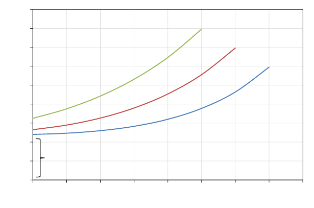
of capital in the credit market, all of which are held fixed. Figure 1 shows stylized
mortgage offer curves for properties with different perceived risk.
4
The mortgage
offer curves are truncated beyond a certain LTV because of credit rationing due
to asymmetric information (Jaffee and Russell, 1976; Leland and Pyle, 1977) and
dead-weight costs of default (Leland, 1994).
Figure 1. Stylized mortgage offer curves for properties with different risk
This figure shows stylized five-year zero-coupon mortgage offer curves for properties with different levels
of perceived risk. Property risk is proxied by annualized asset volatility (“vol”). The vertical axis shows
the mortgage spread over a zero-coupon five-year U.S. Treasury at which lenders would be willing to
issue the mortgage loan given the loan-to-value ratio and the annualized asset volatility. The curves are
computed using the Merton (1974) model and incorporate a liquidity spread, which represents the price
of liquidity in the mortgage-backed securities market.
0.0
0.5
1.0
1.5
2.0
2.5
3.0
3.5
4.0
4.5
50% 55% 60% 65% 70% 75% 80% 85% 90%
Spread (pp)
Loan-to-value ratio
vol = 13%
vol = 17%
vol = 21%
"Liquidity spread"
Given the mortgage offer curve specific to the property, the borrower’s choice
reduces to picking the LTV. In the Leland (1994) model, for example, the optimal
borrower’s choice is decreasing in the property’s cap rate, increasing in the owner’s
4
In this stylized chart, we ignore other mortgage contract terms available to the borrower and
commensurately priced by the lender, including maturity, interim coupon payments, and prepayment
options. We do take such loan features into account in our empirical methodology.
5
tax rate, and decreasing in asset volatility. All else being equal, a model with
rational agents yields equilibrium LTVs that decrease in asset volatility.
There are several key takeaways from the conceptual considerations above.
First, time variation in aggregate LTVs may be entirely attributable to changing
market fundamentals, rather than the tension between regulators and lenders or
agency frictions within lending institutions. Second, in those instances where
LTV limits are below the optimal leverage point for a sufficiently large number
of borrowers, there would be clustering at the credit rationing frontier. Third,
the frontier should decline with perceived property risk. Finally, although lenders
and borrowers do not directly express or observe asset volatility, their risk
assessment is implicit in the loan spread at which the contract is originated.
In Figure 1 above, it is sufficient to know that a loan with a 67% LTV is priced at
2 percentage points above the five-year U.S. Treasury yield to conclude that the
perceived property risk was roughly 17% in implied volatility.
A. Overview of empirical approach and results
Our null hypothesis is that the cross section of LTVs results from borrower
demand in response to rational mortgage offer curves, akin to those depicted in
Figure 1. Under the null hypothesis, it is consistent with prudent lending to provide
an infinitely elastic supply of credit at any point on the curves. Risk misperception
corresponds to lending using offer curves that are systematically lower or higher
than the true asset volatilities, which could be detected ex post. By contrast,
aggressive lending manifests ex ante as loans that would not normally be made
(e.g., an 80% LTV loan with asset volatility of 21% in Figure 1). Hence, one could
test for aggressive lending in a period like 2005–07 by examining whether the
credit rationing frontier was higher during that period than at other times.
5
In order to test the null hypothesis described above, and look for evidence
of aggressive lending practices, we first estimate the implied volatility of each
property underlying a sample of securitized CRE mortgages. The mortgage pricing
model that we use to estimate IV captures various ex ante features of the deal,
including the property’s cap rate, the loan’s term and amortization schedule,
5
Note that changes in the credit rationing frontier could result from the influence of fundamental
factors, such as a systematic change in dead-weight costs of default. Therefore, identifying an epoch with
a higher rationing frontier does not constitute evidence for aggressive lending practices.
6
default and interest rate risk, and mortgage market liquidity.
6
Under the null
hypothesis defined above, IV measures the lender’s perceived property risk. Second,
we identify the credit rationing frontier, as a function of IV, for four time periods
in our sample. We confirm that, consistent with the null hypothesis, the frontier
gradually declines with implied volatility in each of the four periods.
Next, we examine the rationing frontiers and empirically reject the narrative
that lenders were more aggressive in the run-up to the GFC. We use ex ante
fundamentals to explain the variation of LTVs across loans and over time, such
as implied volatility, cap rate, and other property and market features that can
influence mortgage offer curves and borrower demand for loans. We fit a censored
(tobit) regression model for LTV, using the rationing frontier as upper bound,
and conduct a counterfactual analysis. In particular, we fix the frontier over time
and compare actual and estimated counterfactual LTVs to analyze the effect of
changing frontiers. We find little evidence that shifts in the rationing frontier
explain LTVs, which indicates that, even if such shifts are driven by changing
underwriting standards, they have little effect on the distribution of LTVs.
What we do find is that the leading determinant of credit provision is implied
volatility (perceived property risk). Importantly, this relationship is not mechanical.
If borrowers randomly selected LTVs from the mortgage offer curves in Figure 1,
then the only link between LTVs and risk perceptions would be through credit
rationing, because the rationing frontier is more likely to be binding at higher IVs.
This is not consistent with our result that shifts in the rationing frontier explain
little of the distribution of LTVs. By contrast, if borrowers optimally choose LTVs
to trade off costly default against the benefits of debt (e.g., lower taxes), then,
consistent with our empirical findings, LTVs vary with property risk even if the
rationing frontier is not a binding constraint.
B. Literature on commercial real estate risk and mortgage implied volatility
We contribute to an evolving understanding of CRE asset volatility. Previous
analyses use aggregate data to study CRE price dynamics. Ciochetti et al. (2002)
create a property value volatility index at the property type-census district level.
Plazzi, Torous and Valkanov (2010) use quarterly averages at the metropolitan
6
We also examine the possibility that prepayment options affect our results. We confirm that,
because of the presence of large prepayment penalties in this market segment, they do not.
7
statistical area level for broad property types and apply the Campbell and Shiller
(1988) price-dividend decomposition to better understand the characteristics of
CRE rents, cap rates, and asset returns. They find that CRE returns are related
to the local regulatory environment and population density, and that expected
returns are related to factors such as local population, employment, and income
growth as well as construction costs. Using property-level data, we find that many
of these factors are important determinants of asset volatility.
Studies using property-level data have shed light on the magnitude of id-
iosyncratic asset volatility, that is, how much higher asset volatility is than can
be inferred from indexes or other area averages. Plazzi, Torous and Valkanov
(2010) calculate that, aggregated at the metropolitan statistical area-level, the
standard deviation of CRE excess returns ranges from 3.7% to 6.1%, depending
on the property type. By contrast, Downing, Stanton and Wallace (2008) estimate
the asset volatility of CMBS loans using a two-factor Titman and Torous (1989)
model. They find implied volatilities in excess of 20%—higher than our estimates
for their sample period but similar to our post-GFC calculations. Sagi (2021)
uses property-level data from the National Council of Real Estate Investment
Fiduciaries to measure price appreciation volatility. He finds that the standard
deviation of annual price appreciation volatility is about 13%.
7
The mortgage pricing model we use to estimate implied volatility builds on
an extensive body of literature that applies option theoretical methods for pricing
mortgage debt. Some models stipulate a partial differential equation for property
value that is solved using finite difference methods (Titman and Torous, 1989;
Kau et al., 1995). Another popular method, and the one we employ, uses a
binomial model for property valuation (Leung and Sirmans, 1990; Giliberto and
Ling, 1992; Hilliard, Kau and Slawson, 1998; Ciochetti and Vandell, 1999). Similar
to our pricing approach, many of these models incorporate default and prepayment
options. However, while other models assume a single stochastic mean-reverting
interest rate process similar to Cox, Ingersoll and Ross (1985), we model interest
rates using multiple competing models. Furthermore, we include contractual
7
Asset pricing models typically assume that the asset price follows a geometric Brownian motion,
and thus the variance of cumulative price appreciation is linear in the length of the holding period.
Consequently, as the holding period approaches zero, return volatility also approaches zero. By contrast,
Sagi (2021) finds that volatility remains high even for short holding periods. He traces this phenomenon
to transaction risk, finding that the return data fit well to predictions from a search model.
8
characteristics, such as interest-only versus amortizing payment schedules, and
property attributes, such as the cap rate.
Our analysis is closest to that of Downing, Stanton and Wallace (2008).
They also use a two-factor pricing model that prices the mortgage at par, albeit
with the goal to examine the relationship between IVs and CMBS ratings. Similar
to our approach, mortgage value in their model is a function of short rate dynamics
and the property value process. By contrast, our model incorporates a richer set
of loan and property characteristics, including property income and the length
of the interest-only period. Finally, their analysis ends in 2006, while we also
examine developments right before and after the GFC.
C. Evolution of the commercial mortgage-backed securities market
The CRE loans in our data set are CMBS loans: loans originated to be pooled
within Real Estate Mortgage Investment Conduit trusts that issue MBSs. CMBSs
allocate risk among different tranches: the tranches least exposed to credit risk
typically receive investment-grade ratings, while the tranches that absorb credit
losses first are often unrated. In the past two decades, various changes in the
CMBS market affected both the cost of funding and the market for riskier tranches.
In particular, the investor base of riskier tranches changed because of the rise and
fall of CDOs as well as regulatory changes.
Before 2005, unrated tranches were usually held by a set of special
(“B-piece”)
investors, who were involved in security design, performed due diligence, and
selected the servicer responsible for handling delinquencies. In the time period
between 2005 and 2008, it became common practice among CMBS issuers to
repackage such tranches in CRE CDOs. Rating agencies, which made (overly)
optimistic assumptions about the benefits of diversification, assigned favorable
ratings to many CDO tranches. Another factor affecting CMBS markets before
the GFC was a reduction in regulatory capital requirements, as both commercial
bank and investment bank capital requirements for CMBS were reduced in 2004.
Duca and Ling (2020) calculate that commercial bank capital requirements were
reduced from 8% to 2%, while investment bank capital requirements were reduced
from 6% to 3.7%, permitting much higher levels of leverage. As a result, the cost
of funding decreased for both commercial and investment banks, making it easier
for CMBS issuers to sell riskier tranches.
9
After the GFC, CMBS issuance stopped for several years and the CRE
CDO market disappeared. In response to the crisis, regulators increased capital
requirements for commercial banks at the end of 2010, by which time the
major investment banks had been merged with commercial banks. Moreover,
U.S. regulatory agencies proposed Regulation RR, requiring issuers of asset-backed
securities to retain at least five percent of the credit risk, with the intention of
ensuring that issuer incentives are aligned with those of investors.
8
Issuers may
satisfy the risk retention requirement by holding a “vertical” piece of the issued
security, which includes a portion of all tranches, a “horizontal” piece of the
riskiest tranche, or a combination of the two approaches. Although “qualified”
CMBS issuances are exempt from Regulation RR, they are defined in a relatively
conservative manner.
9
Consequently, the risk retention requirement is often
binding for issuers (Flynn Jr, Ghent and Tchistyi, 2020).
Motivated by the substantive variation in the CMBS market and regulatory
environment, we subdivide our sample period into the following four epochs.
1) 2000–04: “B-piece” investors retain the riskiest tranches of CMBSs.
2)
2005–07: CMBS issuers repackage portions of riskier tranches as CRE
CDOs, part of which receive investment-grade ratings. Regulatory capital
requirements associated with CMBS holdings decrease.
3)
2008–15: CMBS issuances plummet then gradually recover to pre-2005 levels.
4) 2016–20: The risk retention rule takes effect in December 2016.
These epoch boundaries are also consistent with the empirical distribution of
CRE loan originations over time. Indeed, as Figure 2 shows, the number of loan
originations exhibits clear cutoffs at the epoch boundaries we use.
8
The risk retention rule was finalized in October 2014 and came into full effect in December 2016.
See https://www.sec.gov/news/pressrelease/2014-236.html for more information.
9
Regulation RR defines a qualifying CRE loan as a fixed-rate loan with a minimum maturity of
10 years and a maximum amortization period of 25 years. Lenders must document property income
for at least the previous two years. The borrower’s debt service ratio must exceed 1.25 for multifamily
properties, 1.5 for leased properties, and 1.7 for all other loans. Furthermore, the combined LTVs of all
loans on the property cannot exceed 70%, and the LTV of the first lien loan cannot exceed 65%.
10
III. Data construction and summary statistics
A. Securitized mortgage loan data collection
Our data consist of 58,127 securitized CRE loans from the year 2000.
10
The data are provided by Morningstar, which gathers information from public
CMBS disclosures, including a rich set of loan and property characteristics.
The Morningstar data include loans originated by a variety of institutions and are
not dominated by a single underwriting approach. Many loans are originated by
large U.S. banks, such as Bank of America and Citibank. The top ten originators
also include large foreign banks, such as Deutsche Bank, Credit Suisse, and UBS.
Non-depository institutions are a substantial part of the market, but no single
such institution has a large market share.
The complete data set consists of 111,465 loans. For the purposes of our
analysis, we drop loans missing key variables needed for our analysis and loans
with problematic observations (see Appendix A for more details). Specifically,
we drop loans that have missing or wrong data for key inputs such as the date of
origination, the loan interest rate, whether the loan is interest-only or amortizing,
and the date of maturity. We also drop non-fixed-rate and pari passu loans, which
our model does not price, as well as agency CMBS loans because the agency
guarantees would distort our implied volatility estimates. Finally, for analytical
and expositional simplicity, we restrict our sample to single-property loans, which
constitute the overwhelming majority of observations.
The data collection process described above results in a sample of 58,127
CRE loans. We present summary statistics for these loans in Table 1 and their
corresponding cross-sectional distributions in Figure F2 of Appendix F. Loans
vary widely in size, from $2 million to over $2.5 billion. LTVs are generally around
70%. The debt yield, the ratio of net operating income (NOI) to loan amount at
origination, varies between 7% and 15%. The debt service coverage ratio (DSCR),
the ratio of NOI to debt servicing amount at origination, falls generally between 1.2
and 2.4. The vast majority (more than 80%) of loans are 10-year loans.
10
Securitized CRE loans are only part of the overall CRE loan market. Black et al. (2017) compare
CMBS loans in the Morningstar data with portfolio CRE loans reported by large U.S. banks on the
FR Y-14 form. They find that these banks are more likely to hold riskier loans, such as construction
loans, in their portfolio. Portfolio loans are also more likely to have floating interest rates, shorter terms,
and lower LTVs than CMBS loans. From their results, it is not clear that securitized and portfolio CRE
loans differ when one sets aside construction loans, which we exclude from our empirical analysis.
11

Table 1—Characteristics of sample commercial real estate loans
This table shows summary statistics for key characteristics of commercial real estate mortgage loans
in our sample, containing fixed-rate, single-property loans securitized in non-agency commercial
mortgage-backed securities (CMBSs). From left to right, the columns show the number of observations
and the sample mean, standard deviation, as well as the 10
th
and 90
th
percentiles of variables in the
cross section of sample loans. At the bottom of the table, the respective spread measures represent
the percentage point yield spreads of sample loans over the 10-year zero-coupon U.S. Treasury yield
and the value-weighted effective yield of the securities constituting the ICE BofA 0-to-3-year AAA
U.S. Fixed-Rate CMBS Index. (Source: ICE Data Indices, LLC, used with permission.)
Count Mean SD P10 P90
Loan amount ($1,000) 58,127 11,465 16,694 2,010 24,260
Loan term (months) 58,127 113 24 83 120
Amortization period (months) 58,127 312 110 0 360
Interest-only period (months) 58,127 21 35 0 60
Loan-to-value ratio 58,127 0.68 0.11 0.55 0.79
Debt yield 58,127 0.11 0.04 0.07 0.15
Debt service coverage ratio 58,127 1.69 0.71 1.18 2.32
Spread over 10-yr U.S. Treasury (pp) 58,127 1.85 0.75 0.92 2.78
Spread over 0-3-yr AAA CMBS (pp) 58,127 1.84 1.17 0.36 3.32
Figure 2 and Table 2 show the distribution of observations over time and
across property types. The volume of loan originations steadily increased until the
GFC, fell to almost zero in 2008, and gradually recovered after 2010. The most
common property types are retail and multifamily, and also a large number of
loans belong to the “other” category.
11
Hotel and industrial properties have the
smallest frequency share in the sample.
We present summary statistics for the properties used as collateral for sample
CRE loans in Table 3. The median property is nine years old and nearly fully leased.
Properties vary widely in size, from 16 thousand to 24 million sqft. Some property-
level variables are unevenly populated, mostly due to heterogeneous measurement
and reporting standards across property types. For instance, information on the
lead tenant is not collected for multifamily properties because they have many
small units, each leased to a different tenant.
11
The “other” category consists of mini-storage and mixed-use properties representing a combination
of property types such as a complex with both multifamily and retail property.
12

Figure 2. Annual number of sample commercial real estate loan originations over time
This figure shows the annual number of commercial real estate mortgage loan originations in our
sample, color coded by time period (epoch). The sample contains fixed-rate, single-property loans
securitized in non-agency commercial mortgage-backed securities. Epoch choice is explained in Section II.C.
0
2,000
4,000
6,000
8,000
2000
2001
2002
2003
2004
2005
2006
2007
2008
2009
2010
2011
2012
2013
2014
2015
2016
2017
2018
2019
2020
Number of Observations Over Time
Table 2—Distribution of sample commercial real estate loans across property types
This table shows the absolute and relative frequencies of commercial real estate mortgage loans in our
sample across different collateral property types. The sample contains fixed-rate, single-property loans
securitized in non-agency commercial mortgage-backed securities.
Property type Count Share
Hotel 4,808 8.3%
Industrial 3,052 5.3%
Multifamily 18,972 32.6%
Office 9,308 16.0%
Other 5,903 10.2%
Retail 16,084 27.7%
Total 58,127 100.0%
In our data filtering, we drop loans with a debt yield less than 0.07 and DSCR
less than 1.25. These lower bounds correspond to standard underwriting limits
(i.e., lenders are reluctant to lend if the debt yield or DSCR is too low) and fall
around the 10
th
percentile in our full sample of CMBS loans. When the debt
yield and DSCR are very low, it may suggest that the property is not currently
13

Table 3—Characteristics of sample commercial real estate loan properties
This table shows summary statistics for key characteristics of the properties used as collateral for
commercial real estate mortgage loans in our sample at the time of loan origination. The sample contains
fixed-rate, single-property loans securitized in non-agency commercial mortgage-backed securities.
From left to right, the columns show the number of observations and the sample mean, standard
deviation, as well as the 10
th
and 90
th
percentiles of variables in the cross section of sample properties.
The area of the property in square feet, as well as the derived variables occupancy rate and lead tenant
share, are available only for industrial, office, retail, and most “other” property types. By commercial real
estate market convention, the size of hotel and multifamily properties is measured by the number of units.
Count Mean SD P10 P90
Property value ($1,000) 58,127 17,524 28,014 3,070 36,000
Net operating income ($1,000) 58,127 1,158 1,771 214 2,335
Area (1,000 sqft) 33,562 112.45 151.08 15.99 240.02
Age (years) 52,569 14.26 15.77 1.00 35.00
Occupancy rate 31,929 0.94 0.10 0.83 1.00
Lead tenant area share 29,333 0.42 0.29 0.12 1.00
Lead tenant lease length (years) 29,832 15.98 240.45 2.17 16.25
stabilized—even if it may be anticipated to be shortly. Since our model uses the
property’s underwritten cap rate as an input, including non-stabilized properties
would distort our implied risk estimate. We are left with 48,468 observations,
which we use throughout our empirical analysis in the paper.
B. Adjustment for capital market liquidity dynamics
One limitation of our mortgage valuation model is that it incorporates only
two dynamic factors: the short interest rate process and the property value process.
However, in practice, Christopoulos (2017) shows that mortgage pricing is also
affected by a time-varying liquidity premium. Therefore, without appropriate
correction, our model would attribute an increase in primary CRE mortgage rates
due to a higher liquidity premium to increased credit risk, which would cause an
upward bias in our volatility estimates.
We take the liquidity premium into account by adjusting loan rates before
the model-based property valuation step. Specifically, we create a monthly time
series of the CMBS liquidity spread by taking the value-weighted effective yield of
securities in the ICE BofA 0-to-3-Year AAA U.S. Fixed-Rate CMBS Index minus
the yield of zero-coupon U.S. Treasury securities with the corresponding effective
14
(i.e., option-adjusted) duration.
12
We then adjust the mortgage rate for each loan
by the prevailing liquidity spread as follows:
(1) r
adj
= r
observed
− (CMBS spread − 120bp),
where 120 basis points is the median value of the CMBS yield spread defined
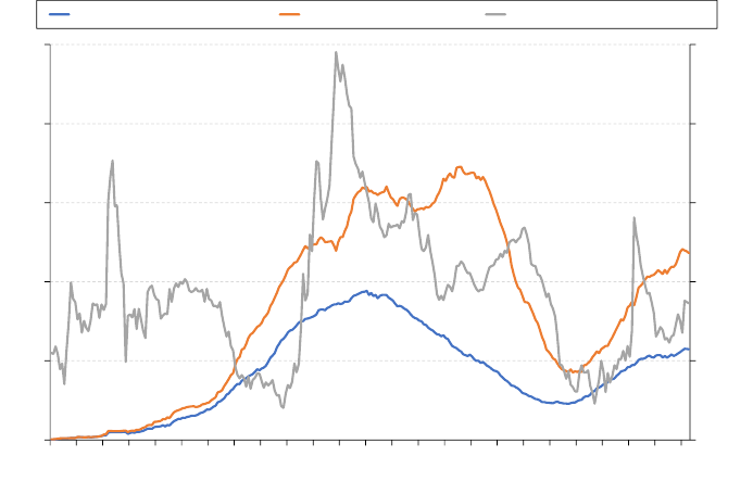
above. Figure 3 shows the yield spread and the number and market value of the
CMBSs with the shortest duration. Although this adjustment leaves a constant
baseline level of liquidity premium embedded in mortgage rates, the remaining
upward bias should permit relative comparisons of perceived property risk over
time based on our model-implied volatilities.
Figure 3. Statistics for 0-to-3-year AAA fixed-rate commercial mortgage-backed securities
This figure shows quarterly aggregates from 1998 to 2022 for the commercial mortgage-backed
securities (CMBSs) constituting the ICE BofA 0-to-3-Year AAA U.S. Fixed-Rate CMBS Index. (Source:
ICE Data Indices, LLC, used with permission.) UST yield spread is defined as the basis point (bp)
difference between the value-weighted mean effective yield of the index constituents over the yield of
the corresponding zero-coupon U.S. Treasury security with maturity equal to the value-weighted mean
effective duration of the index constituents.
32
64
128
256
512
1,024
0
50
100
150
200
250
1998
1999
2000
2001
2002
2003
2004
2005
2006
2007
2008
2009
2010
2011
2012
2013
2014
2015
2016
2017
2018
2019
2020
2021
2022
Number of securities (x10) Market value ($ billion) UST yield spread (bp, right)
12
Source: ICE Data Indices, LLC, used with permission.
15
IV. Implied volatility estimation and diagnostics
We use a two-factor model (with disaster risk) to estimate implied asset
volatility, which we then use as a proxy measure for perceived property risk.
The model ignores correlations between U.S. Treasury yields and property values
and is described in Appendix B. Although there is no standard way to measure
property risk in the presence of market frictions and incompleteness, our implied
volatility estimate is a reasonable measure of risk perception.
13
Figure 4 shows different implied volatility estimates based on our model.
The first IV estimate makes no liquidity adjustments to mortgage rates and does
not consider the effect of prepayment options. The second IV estimate allows
for optimal prepayment in the presence of contractual penalties. Save for 2012,
the presence of prepayment penalties makes little difference in implied volatility.
This is because prepayment penalties, which are ubiquitous in the CRE mortgage
market, are usually sufficiently punitive to render the value of a prepayment
option second-order in mortgage valuation. Notably, given missing data problems
(see Appendix A for further details), ignoring prepayment options in our model
has the advantage of permitting a larger data set. The third IV estimate applies
the liquidity adjustment to mortgage rates discussed in Section III.B and ignores
prepayment options. Adjusting rates for mortgage market liquidity has a profound
effect on the implied measure of property risk. Therefore, because of concerns
raised earlier about risk mismeasurement, we use the liquidity-adjusted implied
volatilities throughout our empirical analysis in the paper.
Figure 5 depicts the distribution of implied volatilities calculated using liquidity
adjustments (and no prepayment options). The time series mean (median) is 20%
(19%) and the standard deviation is 7.5%. The time variation in IVs is pronounced
and corresponds to shifts in the entire distribution, which suggests that perceived
property risk changes systematically over time. It is tempting to expect this time
series variation to coincide with property market cycles, but that need not be the
case because risk perceptions and liquidity on the credit market also affect the
13
The risk-neutral valuation methodology is based on the assumption that contingent claims can
be replicated through self-financing portfolio strategies. Clearly, this assumption does not hold in the
illiquid real estate market. Hence, in some sense, relying on the risk-neutral valuation methodology is
similar to assuming the normality of unobserved shocks in a linear filtering problem. We acknowledge the
limitations of this approach and provide validity and robustness tests, but our IV estimate is ultimately a
proxy measure for, rather than an exact identification of, the property risk perceived by lenders.
16

Figure 4. Sample means of implied volatility estimates over time
This figure shows the cross-sectional means of the estimated model-implied volatilities of commercial real
estate mortgage loans in our sample over time. The sample contains fixed-rate, single-property loans,
with debt yields over 7% and debt service coverage ratios over 1.25, securitized in non-agency commercial
mortgage-backed securities. The implied volatilities are estimated using the two-factor model described
in Appendix B. There are three batches of estimates: a baseline batch without prepayment penalties
or market liquidity adjustment, a batch with prepayment penalties, and a batch with market liquidity
adjustment. The market liquidity adjustment process is explained in Section III.B.
0.00
0.05
0.10
0.15
0.20
0.25
0.30
2000
2001
2002
2003
2004
2005
2006
2007
2008
2009
2010
2011
2012
2013
2014
2015
2016
2017
2018
2019
2020
Baseline Prepayment Liquidity
property market equilibrium. For example, during times of low perceived risk
and high liquidity in credit markets, more properties meet lenders’ and borrowers’
criteria for financing. Hence, the effect of credit market cycles is also reflected in
CRE loan terms and, ultimately, in our volatility estimates.
Indeed, the period with the lowest average IV is 2003–07, which coincides with
the period of the greatest number of CMBS loan originations (Figure 2) and liquid
credit markets. Meanwhile, IVs in 2008–10 are likely biased downward because
lenders extended credit only to the safest properties as credit markets dried up
(Figure 3). By contrast, the highest IVs come from 2001 and 2017–19, which are
periods characterized by relative liquidity in credit markets. Such high IVs are a
function of higher-than-average perceived property risk in the aggregate as well as
an increased willingness by lenders and borrowers to finance riskier assets.
17

Figure 5. Sample quartiles of implied volatilities over time
This figure shows the cross-sectional quartiles of the estimated model-implied volatilities of the commercial
real estate mortgage loans in our sample over time. The sample contains fixed-rate, single-property loans,
with debt yields over 7% and debt service coverage ratios over 1.25, securitized in non-agency commercial
mortgage-backed securities. The implied volatilities are estimated using the two-factor model described in
Appendix B, applying the market liquidity adjustment explained in Section III.B. For lack of observations,
the quartiles cannot be estimated in 2009, when the commercial real estate mortgage market dried up.
0.00
0.05
0.10
0.15
0.20
0.25
0.30
2000
2001
2002
2003
2004
2005
2006
2007
2008
2009
2010
2011
2012
2013
2014
2015
2016
2017
2018
2019
2020
1st Quartile Median 3st Quartile
A. Structural determinants of implied volatility
One potential critique of our use of implied volatility as a proxy for perceived
property risk is the claim that lenders were risk insensitive when setting CRE
loan spreads pre-GFC. In particular, our IVs might capture something other
than property risk in the run-up to the GFC. For instance, pressure to originate
for fees during the height of CDO issuances could have spurred competition for
originating CMBS loans, resulting in exceptionally low mortgage rates, which do
not accurately reflect the true risk of the underlying properties.
We address this critique, and validate the conjecture that implied volatility
is related to structural determinants of property risk, by investigating the pre-
and post-GFC drivers of IV and verifying whether relevant macroeconomic and
property-level risk indicators contributed similarly to risk perceptions over time.
Table 4 examines the pre- and post-crisis relationship between IV (the dependent
18

variable) and various structural variables, such as state GDP, real estate sector
GDP, unemployment rate, and income per capita as well as property size and age.
Property and interacted state and time fixed effects are included. Property age,
state GDP, and state employment rates are positively correlated with risk,
consistent with the findings in Fisher et al. (2022) that urban density is associated
with higher property market risk. Controlling for these variables, we find that
property size and state income levels are negatively related to risk. Importantly,
almost every coefficient that is significant post-GFC is also significant pre-GFC
and has the same sign. If anything, the marginal effects of these variables on IV
are stronger before the crisis than after it.
Table 4—Marginal effects of structural variables on implied volatility (%)
This table shows the estimated marginal effects of relevant local macroeconomic and property-specific
variables on the estimated model-implied volatilities of commercial real estate mortgage loans in our
sample. The sample consists of fixed-rate, single-property loans, with debt yields over 7% and debt service
coverage ratios over 1.25, securitized in non-agency commercial mortgage-backed securities. The marginal
effects are estimated on subsamples before and after the Global Financial Crisis (GFC), using a linear
regression model with the logarithm of implied volatility as dependent variable. The model includes
loan originator, property state, and property type-quarter of origination fixed effects. Standard errors
are double clustered by state and quarter. The implied volatilities are estimated using the two-factor
model described in Appendix B, applying the market liquidity adjustment explained in Section III.B.
Local macroeconomic variables are measured at a quarterly frequency and obtained from the Bureau of
Economic Analysis. “GDP in sector” stands for the gross domestic product of the real estate industry.
Pre-GFC Post-GFC
100 × Log of state real GDP (USD mm) 0.008
∗
0.009
∗∗
100 × Log of state real GDP in sector (USD mm) 0.012 −0.002
100 × Log of state income per capita (USD) −0.045
∗∗
−0.027
∗∗∗
State unemployment rate (%) −0.128 −0.126
∗∗∗
Property Age (years) 0.022
∗∗∗
0.008
∗∗∗
100 × Log of property size (sqft) −0.010
∗∗∗
−0.004
∗∗∗
100 × Log of property size (units) −0.110
∗∗∗
−0.043
∗∗∗
Number of observations 25,493 15,869
∗
p < 0.1,
∗∗
p < 0.05,
∗∗∗
p < 0.01
Additional analysis, not reported here, suggests no significant difference
across IVs based on whether CRE loans were issued by large U.S. banks, smaller
U.S. banks, foreign banks, nonbank lenders, or ex-post acquired or failed lenders.
Overall, we find no empirical evidence that IVs were decoupled from property
fundamentals before the GFC, as compared to the post-GFC period.
19

V. Loan-to-value ratios and risk perceptions
Consistent with a tradeoff theory of optimal firm leverage, Figure 6 shows
that LTV exhibits a strong inverse relationship with implied volatility. Indeed,
a linear regression of IV on LTV yields a far superior fit than a regression on the
other two common CRE mortgage metrics (i.e., DSCR and debt yield). At any
level of perceived property risk, it appears that LTVs were generally highest in
Epoch 1 (2000–04). A notable exception is low-risk loans (with IVs below 15%),
for which the most aggressive period was Epoch 2 (2005–07), when the issuance of
CDOs became prevalent. Interestingly, the same epoch has relatively conservative
LTVs for high-risk loans (with IVs above 20%), while the risk-retention Epoch 4
features slightly higher LTVs than Epoch 3 (2008–15).
Figure 6. Mean loan-to-value ratios across implied volatility bins and epochs
This figure shows the sample means of the loan-to-value ratios (LTVs) of commercial real estate
loans that fall into a given integer bin of model-implied volatility and were originated in a given
time period (epoch). The sample contains fixed-rate, single-property loans, with debt yields over 7%
and debt service coverage ratios over 1.25, securitized in non-agency commercial mortgage-backed
securities. Epoch choice is explained in Section II.C. The implied volatilities are estimated using the two-
factor model described in Appendix B, applying the market liquidity adjustment explained in Section III.B.
0.3
0.4
0.5
0.6
0.7
0.8
0.10 0.15 0.20 0.25 0.30 0.35
Implied Volatility
2000-04 2005-07 2008-15 2016-20
It is important to emphasize that the inverse relationship in Figure 6 is not
tautological. In a frictionless setting, a so-called Modigliani-Miller world, LTV
20
would be arbitrary, and plotting LTVs against IVs would yield no (or a random)
pattern. By contrast, the theories of credit rationing (Jaffee and Russell, 1976;
Leland and Pyle, 1977) and tax benefit–bankruptcy tradeoff (Leland, 1994) predict
a downward-sloping relationship, which we observe empirically.
Figure 6 suggests that there is time variation in leverage choice, even after we
control for perceived property risk. This variation may arise simply from shifts in
the credit rationing frontier, but it may also be due to differences in cap rates or
other, potentially unobserved, property characteristics. In principle, any variable
that affects optimal firm leverage can confound the observed relationship between
LTV and IV. Such variables may include the local credit environment, the marginal
tax rate of investors, and capital expenditure expectations not reflected in cap
rates. In our analysis, we control for such factors and examine their effect on LTV
to gain insight into the evolution of the supply and demand of CRE credit.
A. Credit rationing frontier estimation and diagnostics
In this subsection, we estimate the credit rationing frontier and examine
changes in it over time. Since applying a rationing frontier results in a truncated
distribution of observed LTVs, the observed mean of LTVs moves monotonically
with the truncation point, as long as the distribution of borrower demand is
unchanged. Therefore, a natural question is how much variation in LTV is driven
by changes in the frontier. Our conjecture is that more aggressive lending practices
would primarily be manifested as increases in the rationing frontier.
We define and estimate the rationing frontier as a function of IV, which
shows the maximum amount of leverage that lenders are willing to accept at a
certain level of perceived property risk. Given the scarcity of observations at the
extremes of the distribution, we estimate the frontier only for IVs between 5%
and 40%. The existence of a rationing frontier is clearly visible (see Figure F3 in
the Appendix), with clustering at around 80% LTV for IVs between 5% and 20%.
Using a quantile regression, we estimate the frontier as the 95
th
percentile of LTV
within each 1 percent IV interval (“IV bin”) for each of the four epochs.
14
14
In unreported non-parametric analysis, we verify that the rationing frontier estimate is robust to
the choice of the specific LTV percentile. Furthermore, the 95
th
percentile passes density discontinuity
tests and falls within the cluster of observations lying on the frontier in all four epochs.
21

Figure 7 shows the rationing frontier estimates as a function of IV by epoch.
The 2005–07 epoch stands out in being generally lower than the others. Using the
standard error estimates from our quantile regression, a pairwise mean comparison
across rationing frontier estimates across epochs (see Table 5) shows that the
frontier for this period is, on average, about 4 percentage points lower than the
frontier for the 2000–04 epoch, and about 2 to 3 percentage points lower than the
frontiers after the GFC. This result is contrary to the common belief that lending
standards were lax in the period leading up to the crisis.
Figure 7. Credit rationin g frontier estimates by epoch
This figure shows our credit rationing frontier estimates across periods (epochs). The frontiers are
estimated by fitting a quantile regression model for the 95
th
percentile of the loan-to-value ratios (LTVs) of
commercial real estate loans that fall into a given integer bin of model-implied volatility and were originated
in a given epoch. The estimation sample contains fixed-rate, single-property loans, with debt yields over
7% and debt service coverage ratios over 1.25, securitized in non-agency commercial mortgage-backed
securities. Epoch choice is explained in Section II.C. The implied volatilities are estimated using the two-
factor model described in Appendix B, applying the market liquidity adjustment explained in Section III.B.
0.0
0.1
0.2
0.3
0.4
0.5
0.6
0.7
0.8
LTV
0.00 0.05 0.10 0.15 0.20 0.25 0.30 0.35 0.40
Implied Volatility
2000-04 2005-07 2008-15 2016-20
Overall, our analysis of rationing frontiers does not support a narrative that
CRE lending was more aggressive in the 2005–07 epoch. One possible resolution
for the paradox of low rationing frontier in this epoch is that perceived property
risk was systematically biased downward. Such misperceptions may have led
to excessive supply of credit (e.g., an 80% LTV loan for a property deemed
22

Table 5—Testing mean differences between rationing frontier estimates across epochs
This table shows the results of statistically testing mean differences between rationing frontier estimates
across different periods (epochs). The frontiers are estimated by fitting a quantile regression model
for the 95
th
percentile of the loan-to-value ratios of commercial real estate loans that fall into a given
integer model-implied volatility bin and were originated in a given epoch. The estimation sample
contains fixed-rate, single-property loans, with debt yields over 7% and debt service coverage ratios over
1.25, securitized in non-agency commercial mortgage-backed securities. Epoch choice is explained in
Section II.C. The implied volatilities are estimated using the two-factor model described in Appendix B,
applying the market liquidity adjustment explained in Section III.B. From left to right, the columns
show the mean differences (Diff.), their standard errors (Std. err.), t-statistics, and corresponding p-values.
Frontier pair Diff. Std. err. t-stat p-value
2005–2007 vs. 2000–2004 −0.041 0.0022 −18.64 0.0000
2008–2015 vs. 2000–2004 −0.012 0.0016 −7.86 0.0000
2016–2020 vs. 2000–2004 −0.025 0.0016 −15.22 0.0000
2008–2015 vs. 2005–2007 0.029 0.0023 12.36 0.0000
2016–2020 vs. 2005–2007 0.017 0.0023 7.09 0.0000
2016–2020 vs. 2008–2015 −0.012 0.0018 −6.86 0.0000
to have a volatility of 13% when its volatility is in fact 21%). An alternative
explanation is that loan originators were less risk sensitive when setting mortgage
rates because property risk would affect tranches that were subsequently placed
in CDOs. Although plausible at face value, this alternative is not supported by
our empirical analysis of IV determinants in Section IV, leaving open the question
why credit rationing was tighter in 2005–07.
B. Quantification of loan-to-value ratio determinants
Although we find no empirical support for a laxer credit rationing frontier
before the crisis, it is still useful to examine if shifts in the frontier, which may
be partly driven by imprudent lending practices, have a substantive effect on
the distribution of LTVs. Indeed, based on the analysis of the rationing frontier,
one might argue that the 2000–04 epoch was characterized by lending that was
too permissive. In this section, we analyze the influence of such frontier shifts and,
more broadly, investigate how much of the variation in LTV can be explained by
changes in risk perceptions and property fundamentals.
For our LTV analysis, we introduce the following notation. The demand for
credit by the borrower of loan
i
is
LT V
i
. The amount of credit that is observed to
be extended is
cLT V
i
=
min{R
(
c
i
, b
(
IV
i
))
, LT V
i
}
, where
R
(
c, k
) is the rationing
23
frontier in Epoch
c
and implied volatility bin
k
, as identified in the previous section.
We fit a censored linear regression (tobit) model to cLT V of the form:
(2)
cLT V
i
= max
0, min
R(c
i
, b(IV
i
)),
µ
type
+ µ
s,q
+ o
i
+ α(c
i
)IV
i
+ β
1
CRS
i
+ β
2
CRS
i
2
+ m
m
m
q
γ
γ
γ + ε
i
=
= max
0, min
R(c
i
, b(IV
i
)), x
i
β + ε
i
,
where
µ
type
are property type fixed effects,
µ
s,q
are quarterly time fixed effects and
state/county fixed effects,
o
i
are originator fixed effects,
IV
is implied volatility
(with epoch-specific coefficients), CRS is the cap rate spread over the 10-year
U.S. Treasury yield, and
ε ∼ N
(0
, σ
2
ε
) is the model noise term.
15
Additionally,
m
m
m
q
is a vector of quarterly macro-level variables that we include in model
specifications without time fixed effects.
We present the model coefficient estimates in Table 6, which indicate a strong
negative relationship between LTV and IV. Notably, strictly on its own, and with
a fixed slope coefficient, IV explains two-thirds of LTV variation over time. When
we control for time and property type fixed effects,
2005–07
emerges as the epoch
with the highest sensitivity to IV. This result is also robust to the presence of fixed
effects for the 111 originators in our sample, which suggests that the idiosyncratic
characteristics of individual originators—including those that potentially overstate
property fundamentals, as documented in
Griffin and Priest (2023)
—do not drive
the estimated relationship between LTV and IV. The coefficient of the cap rate
spread is significant and takes the negative sign predicted in Leland (1994).
The CMBS yield spread of short-term AAA CMBS bonds over U.S. Treasury
securities, which measures illiquidity in the mortgage market, accounts for a
large portion of the time series variation in the data. Construed as a cost of
financing, market illiquidity should negatively impact the choice of optimal leverage,
consistent with the sign of its estimated coefficient.
Using the model coefficient estimates, we conduct a counterfactual analysis,
investigating the effect of LTV determinants over time. In particular, we examine
15
The cap rate spread over the 10-year yield is a measure of the cap rate net of the risk-free rate.
Leland (1994) shows that optimal LTV should decline with cap rate. The intuition is that, under the
risk-neutral measure, all assets grow at the same rate (the risk-free rate), so an asset that reinvests income
will grow more than an asset that distributes income. Correspondingly, a slower-growing asset is more
likely to default at loan maturity. We use net cap rate because interest rates experienced a secular decline
between 2000 and 2020, accompanied by a commensurately declining property cap rate.
24

Table 6—Estimation results of censored linear regression for the loan-to-value ratio
This table shows the estimation results of the censored linear regression model defined in Equation
(2)
.
The estimation sample contains fixed-rate, single-property loans, with debt yields over 7% and debt service
coverage ratios over 1.25, securitized in non-agency commercial mortgage-backed securities. The dependent
variable is the loan-to-value ratio, and IV stands for the model-implied volatility estimate for sample loans.
The implied volatilities are estimated using the two-factor model described in Appendix B, applying the
market liquidity adjustment explained in Section III.B. The columns show different model specifications
with an expanding set of explanatory variables and fixed effects included. Standard errors are clustered
by the quarter of loan origination and reported under the corresponding coefficient estimates in parentheses.
(1) (2) (3) (4) (5) (6) (7) (8)
IV -1.28
(0.05)
2000–2004 # IV -1.23 -1.21 -1.46 -1.40 -1.39 -1.38 -1.16
(0.05) (0.05) (0.07) (0.06) (0.06) (0.06) (0.04)
2005–2007 # IV -1.37 -1.32 -1.68 -1.64 -1.61 -1.64 -1.42
(0.05) (0.07) (0.03) (0.03) (0.03) (0.03) (0.06)
2008–2015 # IV -1.37 -1.34 -1.16 -1.29 -1.27 -1.26 -1.17
(0.05) (0.06) (0.03) (0.03) (0.03) (0.03) (0.04)
2016–2020 # IV -1.27 -1.25 -1.23 -1.31 -1.29 -1.28 -1.25
(0.04) (0.05) (0.03) (0.03) (0.03) (0.03) (0.04)
Caprate spread 0.15 -0.07 -0.20 -0.40 -0.43 -0.14
(0.19) (0.13) (0.12) (0.12) (0.12) (0.16)
CMBS yield spread -4.62
(0.73)
UST 10yr yield 0.31
(0.37)
Time (quarterly) x x x
Property type x x x x x
Loan originator x x x x
Property state x
Property state × Time x
Property county x
Generalized R
2
0.61 0.62 0.63 0.71 0.73 0.74 0.76 0.71
Number of observations 45,917 45,917 45,917 45,917 45,917 45,878 45,878 45,779
the effect of shifts in the rationing frontier across epochs on LTVs. To this end,
we estimate counterfactual LTVs, denoted as
cLT V
∗
, setting certain independent
variables in the model constant over time. Formally, we estimate
cLT V
∗
i
= E
n
max
0, min
R(c
∗
i
, b(IV
∗
i
)), LT V
∗
| cLT V
i
,
ˆ
β
β
β, ˆσ
2
ε
,x
x
x
∗
i
o
,(3)
where
cLT V
is the observable,
cLT V
∗
is the censored counterfactual, and
LT V
∗
is the latent counterfactual LTV of the loan,
ˆ
β
β
β
and
ˆσ
2
ε
are the vector of coefficient
estimates and the noise variance estimate from the 8
th
model specification in
Table 6, and
x
x
x
∗
i
is the vector of independent variable values we use for a specific
25
counterfactual scenario. Depending on the observed relation of
cLT V
and the
rationing frontier R, the expression in Equation (3) becomes
(4) cLT V
∗
i
=
max
0, min
R
∗
i
, cLT V
i
+ (x
x
x
∗
i
ˆ
β
β
β − x
x
x
i
ˆ
β
β
β)
if cLT V
i
< R
i
,
E
n
max
0, min
R
∗
i
, LT V
∗
i
o
if cLT V
i
>= R
i
,
where
R
i
=
R
(
c
i
, b
(
IV
i
)) is the original rationing frontier,
R
∗
i
=
R
(
c
∗
i
, b
(
IV
∗
i
))
is the rationing frontier in the counterfactual scenario, and
LT V
∗
i
is the latent
counterfactual LTV of the loan, which follows the truncated normal distribution
N
T R
(x
x
x
∗
i
ˆ
β
β
β, ˆσ
2
ε
) with lower bound R
i
+ (x
x
x
∗
i
ˆ
β
β
β − x
x
x
i
ˆ
β
β
β).
Figure 8 shows the mean LTV in each year of the original data set (Panel A)
and for various counterfactual data sets (Panels B through F). The original data
clearly exhibit a secular decline of LTVs over the sample period. However, this
trend disappears in Panel B, using a counterfactual data set where IV for each
loan is fixed at its sample mean (20%). Further setting the cap rate spread to its
sample mean of 3.7% (Panel C) does not make much difference (consistent with
the estimate in Column 8 of Figure 8). Fixing the CMBS yield spread does appear
to reduce the time series variation (Panel D), while fixing the U.S. Treasury yield
has little effect (Panel E). Importantly, fixing the rationing frontier to correspond
to the first epoch (2000–04) also has little effect on the time series means (Panel F).
Recalling that the first epoch features the most permissive rationing frontier and
the second epoch the least, one might expect a large change in LTVs in the 2005–07
epoch when moving from Panel E to Panel F. Our analysis suggests that shifts in
the rationing frontier have little effect on the distribution of LTVs.
26
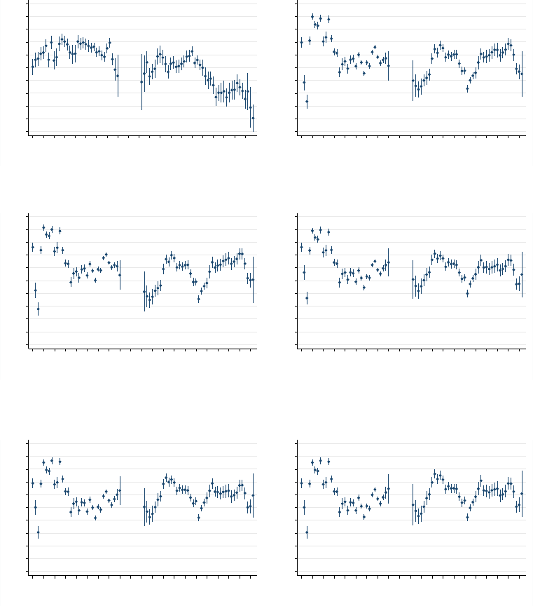
Figure 8. Means of actual and counterfactual loan-to-value ratios over time
This figure shows the means of the actual (Panel A) and counterfactual (rest of the panels) loan-to-value
ratios of commercial lean estate loans in the sample over time, with 99% confidence intervals. The sample
contains fixed-rate, single-property loans, with debt yields over 7% and debt service coverage ratios over
1.25, securitized in non-agency commercial mortgage-backed securities. The counterfactual loan-to-value
ratios are estimated by applying Equation
(3)
and using the 8
th
censored linear model specification in
Table 6. Panels B to F incrementally fix the values of various explanatory variables. UST stands for
the 10-year zero-coupon U.S. Treasury yield, while IV and CRS stand for model-implied volatility and
capitalization rate spread over the UST, respectively.
(a) Actual sample means
0.56
0.58
0.60
0.62
0.64
0.66
0.68
0.70
0.72
0.74
0.76
2000
2001
2002
2003
2004
2005
2006
2007
2008
2009
2010
2011
2012
2013
2014
2015
2016
2017
2018
2019
2020
(Unconditional)
Mean LTVs with 99% CIs
(b) Setting IVs to 20%
0.56
0.58
0.60
0.62
0.64
0.66
0.68
0.70
0.72
0.74
0.76
2000
2001
2002
2003
2004
2005
2006
2007
2008
2009
2010
2011
2012
2013
2014
2015
2016
2017
2018
2019
2020
(Conditional on IV = 20%)
Mean LTVs with 99% CIs
(c) Setting IVs to 20% and CRSs to 370bp
0.56
0.58
0.60
0.62
0.64
0.66
0.68
0.70
0.72
0.74
0.76
2000
2001
2002
2003
2004
2005
2006
2007
2008
2009
2010
2011
2012
2013
2014
2015
2016
2017
2018
2019
2020
(Conditional on IV = 20% and CRS = 370bp)
Mean LTVs with 99% CIs
(d) Setting IVs to 20%, CRSs to 370bp, and
CMBS spread to 120bp
0.56
0.58
0.60
0.62
0.64
0.66
0.68
0.70
0.72
0.74
0.76
2000
2001
2002
2003
2004
2005
2006
2007
2008
2009
2010
2011
2012
2013
2014
2015
2016
2017
2018
2019
2020
(Conditional on IV = 20%, CRS = 370bp, and CMBS = 120bp)
Mean LTVs with 99% CIs
(e) Setting IVs to 20%, CRSs to 370bp,
CMBS spread to 120bp, and UST to 3.2%
0.56
0.58
0.60
0.62
0.64
0.66
0.68
0.70
0.72
0.74
0.76
2000
2001
2002
2003
2004
2005
2006
2007
2008
2009
2010
2011
2012
2013
2014
2015
2016
2017
2018
2019
2020
(Conditional on IV = 20%, CRS = 370bp, CMBS = 120bp, UST10 = 3.2%)
Mean LTVs with 99% CIs
(f) Setting IVs to 20%, CRSs to 370bp,
CMBS spread to 120bp, UST to 3.2%, and fixing
rationing frontier at Epoch 1 level
0.56
0.58
0.60
0.62
0.64
0.66
0.68
0.70
0.72
0.74
0.76
2000
2001
2002
2003
2004
2005
2006
2007
2008
2009
2010
2011
2012
2013
2014
2015
2016
2017
2018
2019
2020
(Conditional on IV = 20%, CRS = 370bp, CMBS = 120bp, UST10 = 3.2%, and Static Frontier)
Mean LTVs with 99% CIs
27

Table 7 compares the annual counterfactual LTV means across the four epochs
and shows that they are statistically distinct. This result means that there is still
statistically significant residual variation across epochs, even after controlling for
IV, cap rate, CMBS spread, U.S. Treasury yield, and changes in the rationing
frontier. That said, the residual time variation does not seem to coincide with
macro events and may rather correspond to shifts in the demand for CRE loans.
Moreover, the residual differences in mean LTV are economically small: less than
three percentage points across all three epochs in Column 6 of Table 7. Notably,
the residual mean differences between Epochs 1 and 4 as well as the difference
between Epochs 2 and 3 are less than one percentage point.
Table 7—Actual and counterfactual means of loan-to-value ratios across epochs
This table shows the means of the actual (Column 1) and counterfactual (rest of the columns) loan-to-value
ratios of commercial lean estate loans in the sample across periods (epochs). The sample contains
fixed-rate, single-property loans, with debt yields over 7% and debt service coverage ratios over 1.25,
securitized in non-agency commercial mortgage-backed securities. The counterfactual loan-to-value ratios
are estimated by applying Equation
(3)
and using the 8
th
censored linear model specification in Table 6.
Each regression, (2)-(6) incrementally fixes the values of various explanatory variables. US10 stands for
the 10-year zero-coupon U.S. Treasury yield, while IV and CRS stand for model-implied volatility and
capitalization rate spread over the US10, respectively. CMBS stands for the market liquidity spread
defined in Section III.B. Robust standard errors are reported in parentheses. At the bottom,
F-statistics
are reported for the joint mean equality tests across Epochs 1 to 4 and Epochs 2 to 4, respectively.
Epoch (1) (2) (3) (4) (5) (6)
2000–2004 68.8 69.4 69.8 69.7 69.1 69.1
(0.1) (0.1) (0.1) (0.1) (0.1) (0.1)
2005–2007 68.7 67.1 68.1 67.1 66.5 66.8
(0.1) (0.0) (0.0) (0.0) (0.0) (0.0)
2008–2015 66.8 66.2 66.6 67.3 67.6 67.8
(0.1) (0.1) (0.1) (0.1) (0.1) (0.1)
2016–2020 62.8 67.6 68.2 67.8 68.1 68.4
(0.1) (0.1) (0.1) (0.1) (0.1) (0.1)
IV = 20% x x x x x
CRS = 370bp x x x x
CMBS = 120bp x x x
US10 = 3.2% x x
Frontier set to Epoch 1 level x
Wald F Stat. of 1–4 equality 587.7 430.4 438.9 403.2 368.1 300.1
Wald F Stat. of 2–4 equality 711.4 109.1 224.1 20.9 175.9 160.9
Number of observations 47,616 45,779 45,779 45,779 45,779 45,779
It is clear from the generalized
R
2
coefficient in Table 6, as well as the
counterfactual LTVs in Figure 8, that the first-order determinant of LTV in
28

the sample is perceived property risk. We assess the individual contribution of
explanatory variables to the cross-sectional variation of LTV
∗
by sequentially
decomposing its sample variance into components of the following form:
(5) VC
n,t
=
Cov
LT V
∗
t
, LT V
∗
t
|
(x
1
,...,x
n−1
)=(¯x
1
,...,¯x
n−1
)
− LT V
∗
t
|
(x
1
,...,x
n
)=(¯x
1
,...,¯x
n
)
V ar
LT V
∗
t
,
where
LT V
∗
t
|
(x
1
,...,x
n
)=(¯x
1
,...,¯x
n
)
denotes the counterfactual latent LTVs in year
t
,
obtained by fixing variables
x
1
to
x
n
at their sample means.
16
Accordingly, the first
variance component is defined as
(5a) VC
1,t
=
Cov
LT V
∗
t
, LT V
∗
t
− LT V
∗
t
|
x
1
=¯x
1
V ar
LT V
∗
t
,
which simplifies to
V ar
(
β
1
x
1
)
/V ar
(
LT V
∗
), which in turn is akin to the
R
2
coefficient of a simple linear regression of
LT V
∗
on
x
1
. Analogously, the residual
variance component is defined as
(5b) VC
ε,t
=
Cov
LT V
∗
t
, LT V
∗
t
|
(x
1
,...,x
n
)=(¯x
1
,...,¯x
n
)
V ar
LT V
∗
t
,
which is the part of variance that cannot be explained with variables x
1
, . . . , x
n
.
In Panel A of Figure 9, we present a variance decomposition in which
x
1
stands
for IV and
x
2
corresponds to all remaining explanatory variables. IV explains
between 40% and 65% of LTV variance in any given year. The incremental
contribution of all other explanatory variables to LTV variance is less than 20%
and averages around 10%. Of these variables, cap rate spread, originator fixed
effects, and geographic fixed effects are the most important determinants of LTV.
We examine their variance contributions in Panel B of Figure 9, which are most
pronounced before the GFC. While originator fixed effects play a relatively more
important role before the crisis, their contribution declines substantially in 2005-07.
16
In essence, we decompose LTV variation using a telescopic sum of counterfactual estimates. Notably,
this decomposition does not ensure that all variance components (VC) are non-negative. Importantly, the
order of the components does not change their values because of the linear core of our tobit model.
29
VI. Conclusion
Theory (e.g., Leland, 1994) suggests that while the choice of optimal firm
leverage depends on both asset and market factors, one of the most important
factors is the risk of the underlying asset. In our empirical anlysis, we demonstrate
that the single most important determinant of LTVs in securitized CRE loans
is perceived property risk, as measured by implied volatility. Indeed, by itself,
IV explains about two-thirds of the variation in LTV. We confirm that other
market-level and asset-specific fundamentals also drive observed choices of LTVs,
albeit explaining less than an additional 10% of LTV variation.
Although LTVs have gradually declined throughout our sample period from
2000 to 2020, the decline disappears once we control for these fundamental factors.
The residual variation does not appear to reflect any market trends. This finding is
relevant because LTV is commonly seen as an important measure of lending stan-
dards and often used in financial regulations
(e.g., DiSalvo and Johnston, 2018)
.
We find some evidence that LTV contains information about lending standards
through shifting maximum LTV criteria (i.e., credit rationing frontiers). However,
the shifts we identify do not support the narrative that lending standards were
lax in the run-up to the GFC. Moreover, we find that changes in frontiers have
had little effect on the distribution of LTVs over time. Finally, we find that IV
was lower in the years before the GFC than at any other period in the past two
decades. A plausible interpretation of this result is that lenders and borrowers
systematically underestimated property risk in this period, leading to excessive
CRE lending and exacerbating the subsequent market downturn.
To the extent that ex ante risk perceptions determine ex post loan performance,
our work motivates the use of measures of market-specific risk perceptions, such as
implied volatility, by both investors and policymakers.
30

Figure 9. Model-based variance decomposition of loan-to-value rati os over time
This figure shows the model-based variance decomposition of the loan-to-value ratios (LTVs) of
commercial lean estate loans in the sample over time. The sample contains fixed-rate, single-property
loans, with debt yields over 7% and debt service coverage ratios over 1.25, securitized in non-agency
commercial mortgage-backed securities. The variance decomposition applies the methodology described
in the text (see Equation
(5)
), measuring the contribution of each variable to the variance of LTV in the
context of the censored linear model defined in Equation
(2)
. More specifically, LTV is modeled using the
8
th
censored linear model specification presented in Table 6. Panel A decomposes the variance of LTV
into the contribution from implied volatility, other model variables, and residual variation. Panel B
presents the variance contribution of the three most relevant model variables other than implied volatility.
(a) Variance attributable to implied volatility and other model variables
0
20
40
60
80
100
2000
2001
2002
2003
2004
2005
2006
2007
2008
2009
2010
2011
2012
2013
2014
2015
2016
2017
2018
2019
2020
1) Contribution of Implied Volatility Variable
2) Incremental Contribution of Other Model Variables
3) Residual Variation
Variance Decompositon of LTVs
(b) Variance attributable to selected other model variables
-2
0
2
4
6
8
10
2000
2001
2002
2003
2004
2005
2006
2007
2008
2009
2010
2011
2012
2013
2014
2015
2016
2017
2018
2019
2020
1) Caprate Spread
2) Loan Originator
3) Property Location
(Contribution of Other Relevant Model Variables)
Variance Decompositon of LTVs
31
REFERENCES
Black, Fischer, and Piotr Karasinski. 1991. “Bond and option pricing when short rates are lognormal.”
Financial Analysts Journal, 47(4): 52–59.
Black, Lamont, John Krainer, Joseph Nichols, et al. 2017. “From Origination to Renegotiation: A
Comparison of Portfolio and Securitized Commercial Real Estate Loans.” The Journal of Real Estate
Finance and Economics, 55(1): 1–31.
Campbell, John Y, and Robert J Shiller. 1988. “Stock prices, earnings, and expected dividends.”
the Journal of Finance, 43(3): 661–676.
CBRE Econometric Advisors. n.d.. “Office, Industrial, Retail, Multi-Housing & Hotel Outlooks.”
https://www.cbre-ea.com/default.aspx?_title=Outlook.
Christopoulos, Andreas D. 2017. “The composition of CMBS risk.” Journal of Banking & Finance,
76: 215–239.
Ciochetti, Brian A. 1997. “Loss Characteristics of Commercial Mortgage Foreclosures.” Journal of
Real Estate Finance, 14(1): 53–69.
Ciochetti, Brian A, and Kerry D Vandell. 1999. “The Performance of Commercial Mortgages.” Real
Estate Economics, 27(1): 27–61.
Ciochetti, Brian A, Yongheng Deng, Bin Gao, and Rui Yao. 2002. “The termination of commercial
mortgage contracts through prepayment and default: a proportional hazard approach with competing
risks.” Real Estate Economics, 30(4): 595–633.
Cox, John C, Jonathan E Ingersoll, and Stephen A Ross. 1985. “A Theory of the Term Structure
of Interest Rates.” Econometrica, 53(2): 385–407.
Cox, John C, Stephen A Ross, and Mark Rubinstein. 1979. “Option pricing: A simplified
approach.” Journal of Financial Economics, 7(3): 229–263.
Curry, Timothy, Joseph Blalock, and Rebel Cole. 1991. “Recoveries on Distressed Real Estate and
The Relative Efficiency of Public versus Private Management.” Real Estate Economics, 19(4): 495–515.
DiSalvo, James, and Ryan Johnston. 2018. “Banking Trends: Skin in the Game in the CMBS
Market.” Economic Insights, 3(1): 11–17.
Downing, Christopher, Richard Stanton, and Nancy Wallace. 2008. “Volatility, mortgage default,
and CMBS subordination.” University of California, Berkeley.
Driessen, Joost, and Otto Van Hemert. 2012. “Pricing of commercial real estate securities during
the 2007–2009 financial crisis.” Journal of Financial Economics, 105(1): 37–61.
Duca, John V, and David C Ling. 2020. “The other (commercial) real estate boom and bust: the
effects of risk premia and regulatory capital arbitrage.” Journal of Banking & Finance, 112: 105317.
Esaki, Howard, Steven L’Heureux, and Mark Snyderman. 1999. “Commercial Mortgage Defaults:
An Update.” Journal of Real Estate Finance, 16(1).
32
Fabozzi, Frank J, Joe McBride, and Manus Clancy. 2015. “The Post-Crisis CMBS Market: Will
Regulations Prevent Another Market Meltdown?” The Journal of Portfolio Management, 41(5): 118–
125.
Fisher, Gregg, Eva Steiner, Sheridan Titman, and Ashvin Viswanathan. 2022. “Location
density, systematic risk, and cap rates: Evidence from REITs.” Real Estate Economics, 50(2): 366–400.
Flynn Jr, Sean J, Andra C Ghent, and Alexei Tchistyi. 2020. “Informational Efficiency in
Securitization after Dodd-Frank.” The Review of Financial Studies, 33(11): 5131–5172.
Giliberto, Michael S, and David C Ling. 1992. “An Empirical Investigation of the Contingent-Claims
Approach to Pricing Residential Mortgage Debt.” Real Estate Economics, 20(3): 393–426.
Griffin, John M, and Alex Priest. 2023. “Is COVID Revealing a Virus in CMBS 2.0?” The Journal
of Finance, Forthcoming.
Gupta, Anurag, and Marti G Subrahmanyam. 2005. “Pricing and hedging interest rate options:
Evidence from cap–floor markets.” Journal of Banking & Finance, 29(3): 701–733.
Hilliard, Jimmy E, James B Kau, and Carlos V Slawson. 1998. “Valuing Prepayment and Default
in a Fixed-Rate Mortgage: A Bivariate Binomial Options Pricing Technique.” Real Estate Economics,
26(3): 431–468.
Hull, John, and Alan White. 1990. “Pricing interest-rate-derivative securities.” The Review of
Financial Studies, 3(4): 573–592.
Jacob, David P, and James M Manzi. 2005. “CMBS Credit Protection and Underwriting Standards.”
The Journal of Portfolio Management, 31(5): 80–90.
Jaffee, Dwight M, and Thomas Russell. 1976. “Imperfect Information, Uncertainty, and Credit
Rationing.” The Quarterly Journal of Economics, 90(4): 651–666.
Kau, James B, Donald C Keenan, Walter J Muller III, and James F Epperson. 1995. “The
valuation at origination of fixed-rate mortgages with default and prepayment.” The Journal of Real
Estate Finance and Economics, 1: 5–36.
Leland, Hayne E. 1994. “Corporate debt value, bond covenants, and optimal capital structure.” The
journal of finance, 49(4): 1213–1252.
Leland, Hayne E, and David H Pyle. 1977. “Informational Asymmetries, Financial Structure, and
Financial Intermediation.” The Journal of Finance, 32(2): 371–387.
Leung, Wai K, and C F Sirmans. 1990. “A Lattice Approach to Pricing Fixed-Rate Mortgages with
Default and Prepayment Options.” Real Estate Economics, 18(1): 91–104.
Levitin, Adam J, and Susan M Wachter. 2013. “The commercial real estate bubble.” Harv. Bus. L.
Rev., 3: 83.
Merton, Robert C. 1974. “On the Pricing of Corporate Debt: The Risk Structure of Interest Rates.”
The Journal of Finance, 29(2): 449–470.
33
Plazzi, Alberto, Walter Torous, and Rossen Valkanov. 2010. “Expected returns and expected
growth in rents of commercial real estate.” The Review of Financial Studies, 23(9): 3469–3519.
Sagi, Jacob S. 2021. “Asset-Level Risk and Return in Real Estate Investments.” The Review of Financial
Studies, 34(8): 3647–3694.
Stanton, Richard, and Nancy Wallace. 2018. “CMBS Subordination, Ratings Inflation, and
Regulatory-Capital Arbitrage.” Financial Management, 47(1): 175–201.
Titman, Sheridan, and Walter Torous. 1989. “Valuing commercial mortgages: An empirical
investigation of the contingent-claims approach to pricing risky debt.” The Journal of Finance,
44(2): 345–373.
Warren, Elizabeth, Paul Atkins, Richard Neiman, Damon Silvers, and J Mark McWatters.
2010. Commercial Real Estate Losses and the Risk to Financial Stability. Government Printing Office.
Wilcox, James A. 2012. “Commercial real estate: Underwriting, mortgages, and prices.” Mortgages,
and Prices (March 15, 2012).
Wilcox, James A. 2018. “An Index of Commercial Real Estate Underwriting: Construction, Causes,
and Effects.”
34
Appendix A: Data construction process
The complete data set consists of 111,465 loans.
•
We remove loans in deals originated by Freddie Mac or Fannie Mae, many
of which finance affordable housing, senior housing, and other subsidized
projects. The pricing of such loans may not fully reflect property risk
perceptions in the commercial real estate mortgage market, partly because of
the embedded guarantee, which our valuation model does not accommodate.
•
We remove loans with missing key variables such as the dates of origination
and maturity, coupon rate, loan amount, net operating income (NOI), and
loan-to-value ratio (LTV). We also drop loans with unrealistic features.
17
•
We only keep loans with debt service coverage ratios above 1.25 and debt
yields above 7%. Our valuation model assumes that dividends, relative to
property value, are constant over the lifetime of the loan. In reality, some
loans finance renovations or other projects that result in NOI increases over
time. Such loans may have projected cash shortfalls at origination, which
would be inconsistent with our structural approach.
•
We have a number of loans for which the call protection lengths plus seasoning
do not add up to the loan term. We have 326 such loans that undershoot the
loan term and 6,908 that overshoot the loan term. When they undershoot,
we extend the last call protection period. When they overshoot, we start
subtracting from the last call protection type, then the second to last, and
so on. For 3,506 loans, the last call protection type is completely removed.
•
We remove a small number of loans that have both defeasance and yield main-
tenance penalties, more than three call protection options, or ambiguous call
protection designations, which our valuation model does not accommodate.
•
We drop 1,850 multi-property and pari passu loans, which our valuation
model does not accommodate.
17
We require coupon rates to be between 1% and 25%, LTVs to be at most 90%, the loan term to be
at most 12 years, and NOI not to exceed the loan amount (i.e., the debt yield to be at most 100%).
35
Appendix B: Implied volatility model
B1. Interest rate process
Gupta and Subrahmanyam (2005) hold a horse race among several pricing
models and find that the accuracy of one-factor models is comparable with that of
other, more complicated, models. We use two of the models they examine: the Hull
and White (1990) (HW) and the Black and Karasinski (1991) (BK) models, which
are among the most commonly used term structure models in practice. We modify
both the HW and BK models so that no more than one tree branch can be above
10% or below zero.
18
This way, we ensure that risk neutral probabilities for the
property price model are positive at property diffusion volatilities as low as 3%.
We note that, during our sample period, forward rates for a one-year zero-coupon
U.S. Treasury bond never exceed 7.5% or fall below 0%. Hence, the bounds we
impose likely reflect market perceptions for the possible range of interest rates
over the lifetime of the mortgages in our data set.
We calibrate each month’s term structure model using yield data obtained for
nominal zero-coupon bonds with maturities ranging from one to twelve years.
19
We obtain data on swaptions with exercise maturity of one year (the most liquid
contracts) from Eikon for tenors (underlying swap maturities) of 1, 5, and 10 years.
Each month, we fit a HW and a BK model to the data and select the one that
best fits the swaptions data.
20
Table B1 summarizes the percentage price accuracy across the fitted monthly
term structure models. Our fitted term structure models are generally accurate.
The BK model seems to be the better performer in roughly 2/3 of cases, and
nearly exclusively so between 2007 and 2015.
18
We modify the HW and BK models as follows. If the conventional HW or BK tree is consistent
with the bounds, we employ it. Otherwise, we truncate all branches beyond the first one that crosses the
bound by setting their transition probabilities to zero. At any node for which branch probabilities are set
to zero, we solve for the remaining branch probabilities by enforcing the node’s expected interest rate
to equal the quantity implied by the underlying mean-reverting process. Generally, the resulting rate
volatility at edge nodes differs from the constant volatility present elsewhere in the tree.
19
We obtain data on yields from the Federal Reserve:
https://www.federalreserve.gov/data/
nominal-yield-curve.htm
. For the short end of the term structure, we use the three-month U.S. Treasury
constant maturity yields calculated by the Federal Reserve of St. Louis.
20
Both the HW and BK models can be made to fit any arbitrary term structure of zero-coupon bonds.
36

Table B1—Term Structure Model Precision
This table shows the accuracy of 277 “best-fitting” term structure models, estimated for each month
from June 1997 to June 2020. The two models used for estimation are the Hull and White (1990) and
the Black and Karasinski (1991) models. Each data point constitutes the root of the weighted mean of
squared pricing errors (i.e., percentage accuracy) from a single month’s term structure model.
Statistic Model precision
Mean 0.0202
SD 0.0439
P1 0.0001
P5 0.0003
P10 0.0007
P25 0.0015
P50 0.0042
P75 0.0149
P90 0.0534
P95 0.1146
P99 0.2322
B2. Property value process
We model property values using a binomial process similar to that in Cox,
Ross and Rubinstein (1979), but modified to incorporate time-varying short-term
interest rates as well as a “catastrophic drop” in value that triggers immediate
default. The latter modification is motivated by the actual distribution of creditor
losses. Without the possibility of a sudden drop (discontinuous downward jump)
in property value, the optimal exercise of the default option tends to predict
relatively small loan losses to what we observe in practice. The catastrophic
property-level event is Poisson distributed and arrives with annual intensity of
λ
. In our model, the event permanently reduces the property’s value to zero,
and the rate λ is calibrated to our loan pool to match historical commercial real
estate (CRE) loss given default (LGD) rates of 30–35%.
21
Let
σ
be the annual volatility of the property’s value. We incorporate
catastrophic hazard in the model of Cox, Ross and Rubinstein (1979) by dividing
21
This range is based on estimates by Esaki, L’Heureux and Snyderman (1999), Ciochetti (1997), and
Curry, Blalock and Cole (1991). One could potentially model a distribution of catastrophic losses, but it
is unclear to what extent this would make our results more reflective of lender perceptions versus a fixed
LGD value. See Appendix D for further elaboration on methodology.
37

the usual “up” and “down” states by (1 − λ∆t) for each ∆t time increment:
u =
e
σ
√
∆t
1 − λ∆t
d =
e
−σ
√
∆t
1 − λ∆t
.
The property value changes by a factor of
u
or
d
. This specification keeps
the expected price appreciation of the property, under the risk-neutral measure,
independent of the value of
λ
and thus independent of the idiosyncratic event.
It also has the virtue of setting the Arrow-Debreu prices of “up” and “down”
non-disaster states equal to (1
− λ
∆
t
) times their usual values in the Cox model:
π
(u)
j,t,k
=
e
r
k,t
∆t
− d(1 − λ∆t)
u − d
π
(d)
j,t,k
=
u(1 − λ∆t) − e
r
k,t
∆t
u − d
,
where we denote property state
j
, time
t
, and continuously compounded short
interest rate state
k
obtained from the term structure model. We assume that
a one-period binomial “up” or “down” move in the property price process is
uncorrelated with the one-period short-term interest rate process.
CRE properties generate income for their owners, which we incorporate by
assuming that the property pays a constant annual “dividend” rate
δ
t
corresponding
to the property’s net cash-flow-to-value ratio (NCF) at the time of mortgage
origination.
22
We include the dividend in our property value process, except
for the time of origination, when the property’s value is equal to the appraised
value. We define “up” and “down” cum-dividend property value
V
j,t+1
for all
non-origination periods t ∈ {1, ..., T − 1} recursively as follows:
V
j
u
,t+1
= uV
j,t
(1 − δ
t
∆t) V
j
d
,t+1
= dV
j,t
(1 − δ
t
∆t).
B3. Valuation of commercial real estate mortgages
We employ a structural mortgage valuation model to estimate the property’s
annual volatility parameter
σ
, which is otherwise not observable. Mortgage terms
comprise the LTV (or, equivalently, the amount borrowed), the time to maturity,
and the amortization schedule. Together with a complete specification of the
property and interest rate model parameters, the mortgage terms imply a fair
22
In the numerator, we use NCF instead of NOI because net cash flow takes capital expenditures and
capital expenditure reserves into account and is arguably a better measure of property cash flows.
38
market mortgage rate that can be calculated by setting the present value of the
mortgage obligation equal to the amount borrowed. Using the model, we solve for
the implied volatility that sets the present value of the mortgage obligation to the
amount borrowed given the observed mortgage rate.
We denote property value
V
j,t,k
(which is
V
j,t
because property value is
independent of interest rate movement), as well as corresponding equity and debt
values,
E
j,t,k
and
D
j,t,k
, respectively. We allow for interest-only or amortizing
mortgage payment schedules (or a combination of these). We denote the remaining
mortgage balance
B
t
and the fixed mortgage payment or coupon
c
t
. As in Cox, Ross
and Rubinstein (1979), we specify our model working backwards from maturity.
Similar to Merton (1974), we define borrower equity and debt at maturity T :
E
j,T,k
= max(0, V
j,T
− (B
T
+ c
T
))
D
j,T,k
= min(V
j,T
, B
T
+ c
T
).
These formulas capture the notion of “mechanical” default: the borrower
defaults if the property value falls below the debt value. Notably, the Modigliani–
Miller value additivity holds:
D
j,t,k
+
E
j,t,k
=
V
j,t,k
, as we prove in Appendix C,
which implies that there is no dead-weight cost to default.
23
There is no prepayment
or dividend payment at maturity. Consequently, for each non-maturity and
non-origination period
t ∈ {
1
, ..., T −
1
}
, the following equations determine the
borrower’s value of equity and debt:
E
j,t,k
= max
0, δ
t
∆tV
j,t,k
− c
t
+
e
−r
k,t
∆t
E
j,t,k
h
˜
E
t+1
i
, V
j,t,k
− c
t
− B
t
− P
j,t,k
D
j,t,k
= min
V
j,t,k
, c
t
+
e
−r
k,t
∆t
E
j,t,k
h
˜
D
t+1
i
, c
t
+ B
t
+ P
j,t,k
,
where
E
j,t,k
[
˜
E
t+1
] and
E
j,t,k
[
˜
D
t+1
] respectively stand for the risk-neutral expected
values for equity and debt, and
P
j,t,k
is the prepayment penalty. The terms in
each equation represent values for default, continuation, and prepayment options.
23
We opt to ignore the dead-weight cost of default because we do not correspondingly model tax
benefits of debt or investors with heterogeneous private values. If mortgage debt came only with costs
and no benefits, then no rational investor would finance a property with mortgage debt.
39
For simplicity, we define the risk-neutral expected values of X ∈ {E, D}:
E
j,t,k
h
˜
X
t+1
i
= π
(u)
j,t,k
h
i
(u)
k,t
X
j
u
,t+1,k
u
+ i
(m)
k,t
X
j
u
,t+1,k
+ i
(d)
k,t
X
j
u
,t+1,k
d
i
+
π
(d)
j,t,k
h
i
(u)
k,t
X
j
d
,t+1,k
u
+ i
(m)
k,t
X
j
d
,t+1,k
+ i
(d)
k,t
X
j
d
,t+1,k
d
i
,
with
i
(u)
k,t
,
i
(m)
k,t
, and
i
(d)
k,t
being interest rate up, middle, and down state probabilities,
respectively. At origination (i.e.,
t
= 0), the values of equity and debt are equal
to their respective continuation values,
E
0
= (
e
−r
0
∆t
)
E
0,0,0
[
˜
E
t+1
] and
D
0
=
(
e
−r
0
∆t
)
E
0,0,0
[
˜
D
t+1
], based on the assumption that there are no coupon payments
or dividends at origination. Given the other model parameters, we estimate the
property’s annual implied volatility by computing the volatility parameter
σ
that
sets D
0
equal to the contractual loan amount.
Prepayment rules are specified in the mortgage covenant and usually vary
by mortgage period. For instance, a common feature is a prepayment lockout of
several months until prepayment is allowed, followed by a lengthy period when
prepayment is allowed but with penalties (usually defeasance or yield maintenance),
followed by another, shorter period when prepayment is allowed without penalties
(the “open” prepayment period). These periods sum to the length of the mortgage.
Accordingly, as described Appendix E in more detail, we model prepayments as
follows: we remove the prepayment option during the lockout period, then explicitly
model defeasance or yield maintenance during penalty period, and finally set
P
j,t,k
equal to zero during the open prepayment period.
40

Appendix C: Proof of Modigliani–Miller additivity
We would like to show that the Modigliani–Miller additivity
E
j,t,k
+
D
j,t,k
=
V
j,t,k
holds for all t ∈ {0, ..., T }.
Part 1 of Proof
We begin by demonstrating that
V
j,t,k
=
δ
t
∆
tV
j,t,k
+ (
e
−r
k,t
∆t
)
E
j,t,k
[
˜
V
t+1
]
for
t ∈ {
1
, ..., T −
1
}
. We redefine the following (note that
V
j,t
=
V
j,t,k
since the
property value is independent of interest rate movements):
V
j
u
,t+1,k
= uV
j,t,k
(1 − δ
t
∆t)
V
j
d
,t+1,k
= dV
j,t,k
(1 − δ
t
∆t)
for t ∈ {1, ..., T − 1}.
We use these to show that V
j,t,k
= δ
t
∆tV
j,t,k
+
e
−r
k,t
∆t
E
j,t,k
h
˜
V
t+1
i
:
δ
t
∆tV
j,t,k
+
e
−r
k,t
∆t
E
j,t,k
h
˜
V
t+1
i
= δ
t
∆tV
j,t,k
+
e
−r
k,t
∆t
h
π
(u)
j,t,k
V
j
u
,t+1,k
+ π
(d)
j,t,k
V
j
d
,t+1,k
i
= δ
t
∆tV
j,t,k
+
e
−r
k,t
∆t
h
π
(u)
j,t,k
uV
j,t,k
(1 − δ
t
∆t) + π
(d)
j,t,k
dV
j,t,k
(1 − δ
t
∆t)
i
= V
j,t,k
δ
t
∆t + (1 − δ
t
∆t)
e
−r
k,t
∆t
π
(u)
j,t,k
u + π
(d)
j,t,k
d
| {z }
= e
r
k,t
∆t
(No Arbitrage)
= V
j,t,k
δ
t
∆t + (1 − δ
t
∆t)
e
−r
k,t
∆t
)(e
r
k,t
∆t
= V
j,t,k
[δ
t
∆t + 1 − δ
t
∆t] = V
j,t,k
.
Part 2 of Proof
At maturity T , the Modigliani–Miller additivity clearly holds because:
E
j,T,k
= max(0, V
j,T
− (B
T
+ c
T
)),
D
j,T,k
= min(V
j,T
, B
T
+ c
T
).
41

We show that M&M holds at any arbitrary time
t ∈ {
1
, ..., T −
1
}
. Assuming
E
j,t+1,k
+ D
j,t+1,k
= V
j,t+1,k
(true for t + 1 = T ) and using induction, we get:
E
j,t,k
= max
0, δ
t
∆tV
j,t,k
− c
t
+
e
−r
k,t
∆t
E
j,t,k
h
˜
E
t+1
i
, V
j,t,k
− c
t
− B
t
− P
j,t,k
,
D
j,t,k
= min
V
j,t,k
, c
t
+
e
−r
k,t
∆t
E
j,t,k
h
˜
D
t+1
i
, c
t
+ B
t
+ P
j,t,k
.
By hypothesis,
E
j,t+1,k
+
D
j,t+1,k
=
V
j,t+1,k
. Therefore, the continuation state
value of date t equity equals:
δ
t
∆tV
j,t,k
− c
t
+
e
−r
k,t
∆t
E
j,t,k
h
˜
E
t+1
i
=
δ
t
∆tV
j,t,k
+
e
−r
k,t
∆t
E
j,t,k
h
˜
V
t+1
i
| {z }
=V
j,t,k
by Result 1
−c
t
−
e
−r
k,t
∆t
E
j,t,k
h
˜
D
t+1
i
= V
j,t,k
− c
t
−
e
−r
k,t
∆t
E
j,t,k
h
˜
D
t+1
i
,
which implies that:
E
j,t,k
= max
0, V
j,t,k
− c
t
−
e
−r
k,t
∆t
E
j,t,k
h
˜
D
t+1
i
, V
j,t,k
− c
t
− B
t
− P
j,t,k
= V
j,t,k
+ max
−V
j,t,k
|
{z }
−x
j,t,k
, −c
t
−
e
−r
k,t
∆t
E
j,t,k
h
˜
D
t+1
i
| {z }
−y
j,t,k
, −c
t
− B
t
− P
j,t,k
| {z }
−z
j,t,k
.
In conclusion:
E
j,t,k
+ D
j,t,k
= V
j,t,k
+ max(−x
j,t,k
, −y
j,t,k
, −z
j,t,k
)+
+ min(x
j,t,k
, y
j,t,k
, z
j,t,k
) = V
j,t,k
.
42

We can easily show that the additivity holds at
t
= 0 as well. Taking the
appraised property value at origination S
0
, we divide by (1 − δ
t
∆t) to get V
0
.
E
0
= (e
−r
0
∆t
)
E
0,0,0
[
˜
E
t+1
],
D
0
= (e
−r
0
∆t
)
E
0,0,0
[
˜
D
t+1
],
V
0
=
S
0
(1 − δ
t
∆t)
⇔ S
0
= V
0
− δ
t
∆tV
0
.
Using the continuation values of equity and debt for
t ∈ {
1
, ..., T −
1
}
referenced
earlier and removing the dividend δ
t
∆tV
0
and coupon c
t
, we get:
E
0
= S
0
− (e
−r
0
∆t
)
E
0,0,0
[
˜
D
t+1
],
E
0
+ D
0
= S
0
− (e
−r
0
∆t
)
E
0,0,0
[
˜
D
t+1
] + (e
−r
0
∆t
)
E
0,0,0
[
˜
D
t+1
] = S
0
.
Appendix D: Loss given default
We define LGD at each default node j, t, k as follows:
LGD
j,t,k
= 1 −
V
j,t,k
c
t
+ B
t
.
For each loan in our sample, we obtain an expected LGD figure using 10,000
Monte Carlo simulations. We do this by generating random property and interest
rate trajectories and weighting them by their respective risk-neutral probabilities.
Upon reaching a default node, the simulation stops and records LGD for simulation
number
i
as
LGD
i
=
LGD
j,t,k
. If no default occurs,
LGD
i
= 0. With probability
λ
∆
t
, a catastrophic property loss happens (the risk-neutral “up” and “down”
property probabilities sum to 1
− λ
∆
t
) and default occurs with
LGD
i
= 1.
Therefore, the expected LGD for each loan l is:
eLGD
l
=
Σ
10000
i=1
LGD
i
/10000.
43
Appendix E: Prepayment penalties
We use the standard concepts of defeasance and yield maintenance, with small
modifications to accommodate our term structure models.
The basic principle of defeasance is that the lender charges a penalty for the
spread that it loses when the borrower refinances the loan. We model this spread
by using our term structure calculations to create a portfolio of risk-free assets
(zero-coupon bonds, ZCB) with the same cash flows. The calculation for any
interest rate state k, t is as follows:
Def
k,t
=
T −t
X
i=1
m
t+i
ZCB
k,t,t+i
!
− B
t
,
where
m
t+i
is the mortgage payment at date
t
+
i
,
ZCB
k,t,t+i
is the value at date
t
of a zero-coupon bond with maturity at date
t
+
i
, and
B
t
is the remaining mortgage
balance.
24
ZCB
k,t,t+i
is calculated by creating a sub-tree
M
of all continuation
states starting at node
k, t
of the trinomial interest rate tree. The final column of
the tree, which represents time
t
+
i
, has payoffs of 1 (
M
k,t+i+1
= 1
∀k
). We then
determine the zero-coupon bond price by iterating backwards to the original node
(k, t) so that the following recursive formula holds:
M
k,t
=
e
−r
k,t
∆t
h
i
(u)
k,t
M
k
u
,t+1
+ i
(m)
k,t
M
k
m
,t+1
+ i
(d)
k,t
M
k
d
,t+1
i
.
Yield maintenance differs from defeasance in that it replaces the lost spread
with a risk-free asset of the same remaining term as the original loan. We model
yield maintenance by using the zero-coupon bond rates calculated above. First,
we calculate the “risk-free” par bond rate for the appropriate maturity:
rf
k,t
= (1 − ZCB
k,t,T
) /
T −t
X
i=1
ZCB
k,t,t+i
!
.
24
For simplicity, we calculate defeasance and yield maintenance up to maturity
T
. In practice,
there is heterogeneity across lenders, with some calculating the penalty up to the beginning of the open
prepayment period instead. Although we do not observe the exact lender method in our data, the
differences between the beginning of the open prepayment period and maturity are typically very small.
44
Then, we calculate an annual “present value factor” f:
f
k,t
=
(1 − (1 + rf
k,t
))
−(T −t)/∆t
/ rf
k,t
.
Finally, the yield maintenance penalty is calculated:
Y M
k,t
= (rm − rf
k,t
) f
k,t
B
t
,
where rm is the mortgage rate.
45

Appendix F: Additional figures and tables
Table F1—Distribution of CRE Loans by Property Type
This table shows the absolute frequencies of commercial real estate mortgage loans in the Morningstar
data set across different collateral property types, with an emphasis on the distinctions between single
and multi-property loan frequencies. The sample contains fixed-rate loans, with debt yields over 7%
and debt service coverage ratios over 1.25, securitized in non-agency commercial mortgage-backed securities.
Single-Property Loans Multi-Property Loans Total
Hotel 4,808 194 5,002
Industrial 3,052 133 3,185
Mixed 0 174 174
Multifamily 18,972 491 19,463
Office 9,308 215 9,523
Other 5,903 331 6,234
Retail 16,084 292 16,376
Total 58,127 1,830 59,957
Table F2—Extreme Percentiles of Implied Volatility Estimates by Epoch
This table shows the lowest and highest three percentiles of implied volatility estimates by period
(epoch). Epoch choice is explained in Section II.C. The implied volatilities are estimated using the
two-factor model described in Appendix B, applying the market liquidity adjustment explained
in Section III.B. The sample contains fixed-rate, single-property loans, with debt yields over 7%
and debt service coverage ratios over 1.25, securitized in non-agency commercial mortgage-backed securities.
P1 P2 P3 P97 P98 P99
2000–2004 0.06 0.08 0.09 0.36 0.39 0.44
2005–2007 0.08 0.09 0.10 0.32 0.34 0.39
2008–2015 0.06 0.08 0.09 0.32 0.34 0.37
2016–2020 0.10 0.12 0.13 0.36 0.38 0.40
Entire sample 0.07 0.08 0.09 0.34 0.36 0.40
46

Figure F1. Distribution of Implied Volatility by Epoch
This figure shows the distribution of implied volatility estimates by period (epoch). Epoch choice is
explained in Section II.C. The implied volatilities are estimated using the two-factor model described in
Appendix B, applying the market liquidity adjustment explained in Section III.B. The sample contains
fixed-rate, single-property loans, with debt yields over 7% and debt service coverage ratios over 1.25,
securitized in non-agency commercial mortgage-backed securities.
(a) 2000–2004
0
20
40
60
80
100
0
2
4
6
8
10
0 10 20 30 40 50 60 70
Implied Volatility (%)
(b) 2005–2007
0
20
40
60
80
100
0
2
4
6
8
10
0 10 20 30 40 50 60 70
Implied Volatility (%)
(c) 2008–2015
0
20
40
60
80
100
0
2
4
6
8
10
0 10 20 30 40 50 60 70
Implied Volatility (%)
(d) 2016–2020
0
20
40
60
80
100
0
2
4
6
8
10
0 10 20 30 40 50 60 70
Implied Volatility (%)
47

Figure F2. Distribution of Selected CRE Loan Characteristics
This figure shows the distribution of debt service coverage ratios, debt yield, loan-to-value ratios, and loan
term lengths in the Morningstar data set of fixed-rate, single-property loans securitized in non-agency
commercial mortgage-backed securities. The sample is later cut for further analysis by removing debt
yields under 7% and debt service coverage ratios under 1.25 for reasons explained in Section III.A.
(a) DSCR
0
10
20
30
0 1 2 3 4 5
(b) Debt Yield
0
5
10
15
20
0.00 0.05 0.10 0.15 0.20 0.25
(c) Loan-to-Value Ratio
0
10
20
30
0.0 0.1 0.2 0.3 0.4 0.5 0.6 0.7 0.8 0.9
(d) Loan Term (Month)
0
20
40
60
80
0 12 24 36 48 60 72 84 96 108 120 132 144
48

Figure F3. Association Between the LTVs and IVs of CMBS Loans Over Different Epochs
This figure shows the relationship between loan-level loan-to-value ratios and implied volatility estimates
by period (epoch). Epoch choice is explained in Section II.C. The implied volatilities are estimated using
the two-factor model described in Appendix B, applying the market liquidity adjustment explained in
Section III.B. The overlaid frontiers are estimated by fitting a quantile regression model for the 95
th
percentile of the loan-to-value ratios (LTVs) of commercial real estate loans that fall into a given integer
bin of model-implied volatility and were originated in a given epoch. The samples contain fixed-rate,
single-property loans, with debt yields over 7% and debt service coverage ratios over 1.25, securitized in
non-agency commercial mortgage-backed securities.
(a) 2000–2004 (b) 2005–2007
(c) 2008–2015 (d) 2016–2020
49

Table F3—Marginal Effects of Explanatory Variables on 100 × Log of Implied Volatility
This table shows the marginal effects of these explanatory variables on 100
×
log of implied volatility. The implied volatilities are estimated using
the two-factor model described in Appendix B, applying the market liquidity adjustment explained in Section III.B. The samples contain fixed-rate,
single-property loans, with debt yields over 7% and debt service coverage ratios over 1.25, securitized in non-agency commercial mortgage-backed securities.
Property size is measured alternatively in square feet and “units” by Morningstar. Rather than attempt a conversion, we utilize either of these variables
when it is available. Certain variables are heterogeneously populated among property types, motivating us to include and exclude hotel, multifamily, and
“other” property types in the various columns. GDP, income, and unemployment data are obtained from the Bureau of Economic Analysis (BEA). “Sector”
refers to the “real estate industry” as defined by the BEA. The market size and vacancy rate data are obtained from CBRE Econometric Advisors.
(1) (2) (3) (4) (5)
100 × Log of State Real GDP (USD mm) 0.02 0.07 -0.00
100 × Log of State Real GDP in Sector (USD mm) 0.05 -0.03 -0.01
100 × Log of State Income per Capita (USD) -0.20
∗
-0.11 -0.06
State Unemployment Rate (%) -1.36
∗∗
-1.19
∗
-1.20
∗∗
Property Age (Years) 0.08
∗∗∗
0.08
∗∗∗
0.08
∗∗∗
0.05
∗
0.05
∗∗
100 × Log of Property Size (Sqft) -0.04
∗∗∗
-0.04
∗∗∗
-0.04
∗∗∗
-0.04
∗∗∗
-0.03
∗∗∗
100 × Log of Property Size (Units) -0.42
∗∗∗
-0.42
∗∗∗
-0.39
∗∗∗
Property Occupancy (%) -0.10
∗∗∗
-0.16
∗∗∗
Lead Tenant Share (%) 0.05
∗∗∗
0.05
∗∗∗
100 × Log of Market Size (Sqft) 0.03
∗∗∗
0.01
Market Vacancy Rate (%) -0.03 0.27
∗∗∗
Hotel Included x x x
Multifamily Included x x x
Other Included x x x
Loan Originator x x x x x
Property State x x x
Property Type × Time (Quarterly) x x x x x
Property County × Time (Quarterly) x x
R
2
0.37 0.31 0.38 0.51 0.54
Number of Observations 41,362 19,626 26,433 13,185 21,209
Standard errors are double clustered by the property state and the quarter of origination.
∗
p < 0.1,
∗∗
p < 0.05,
∗∗∗
p < 0.01
50

Table F4—Marginal Effects of Explanatory Variables on Implied Volatility (%)
This table shows the marginal effects of these explanatory variables on percentage implied volatility. The implied volatilities are estimated using
the two-factor model described in Appendix B, applying the market liquidity adjustment explained in Section III.B. The samples contain fixed-rate,
single-property loans, with debt yields over 7% and debt service coverage ratios over 1.25, securitized in non-agency commercial mortgage-backed securities.
Property size is measured alternatively in square feet and “units” by Morningstar. Rather than attempt a conversion, we utilize either of these variables
when it is available. Certain variables are heterogeneously populated among property types, motivating us to include and exclude hotel, multifamily, and
“other” property types in the various columns. GDP, income, and unemployment data are obtained from the Bureau of Economic Analysis (BEA). “Sector”
refers to the “real estate industry” as defined by the BEA. The market size and vacancy rate data are obtained from CBRE Econometric Advisors.
(1) (2) (3) (4) (5)
100 × Log of State Real GDP (USD mm) 0.004 0.013 -0.001
100 × Log of State Real GDP in Sector (USD mm) 0.009 -0.006 -0.002
100 × Log of State Income per Capita (USD) -0.037
∗
-0.020 -0.011
State Unemployment Rate (%) -0.253
∗∗
-0.223
∗
-0.221
∗∗
Property Age (Years) 0.014
∗∗∗
0.015
∗∗∗
0.014
∗∗∗
0.010
∗
0.010
∗∗
100 × Log of Property Size (Sqft) -0.007
∗∗∗
-0.007
∗∗∗
-0.007
∗∗∗
-0.007
∗∗∗
-0.006
∗∗∗
100 × Log of Property Size (Units) -0.077
∗∗∗
-0.077
∗∗∗
-0.071
∗∗∗
Property Occupancy (%) -0.019
∗∗∗
-0.029
∗∗∗
Lead Tenant Share (%) 0.010
∗∗∗
0.009
∗∗∗
100 × Log of Market Size (Sqft) 0.005
∗∗∗
0.002
Market Vacancy Rate (%) -0.005 0.050
∗∗∗
Hotel Included x x x
Multifamily Included x x x
Other Included x x x
Loan Originator x x x x x
Property State x x x
Property Type × Time (Quarterly) x x x x x
Property County × Time (Quarterly) x x
Number of Observations 41,362 19,626 26,433 13,185 21,209
Standard errors are double clustered by the property state and the quarter of origination.
∗
p < 0.1,
∗∗
p < 0.05,
∗∗∗
p < 0.01
51

Table F5—Marginal Effects of Explanatory Variables on IV (%)
This table shows the marginal effects of these explanatory variables on percentage implied volatility.
The implied volatilities are estimated using the two-factor model described in Appendix B, applying
the market liquidity adjustment explained in Section III.B. This sample contain fixed-rate, single-
property loans, with debt yields over 7% and debt service coverage ratios over 1.25, securitized in
non-agency commercial mortgage-backed securities. This sample excludes hotel and multifamily properties.
Pre-GFC Post-GFC
Property Age (Years) 0.009
∗
0.012
100 × Log of Property Size (Sqft) -0.008
∗∗∗
-0.004
∗∗∗
Property Occupancy (%) -0.025
∗∗∗
-0.072
∗∗∗
Lead Tenant Share (%) 0.006
∗∗
0.027
∗∗∗
Number of Observations 10,573 2,612
∗
p < 0.1,
∗∗
p < 0.05,
∗∗∗
p < 0.01
Table F6—Marginal Effects of Explanatory Variables on IV (%)
This table shows the marginal effects of these explanatory variables on percentage implied volatility. The
implied volatilities are estimated using the two-factor model described in Appendix B, applying the
market liquidity adjustment explained in Section III.B. This sample contain fixed-rate, single-property
loans, with debt yields over 7% and debt service coverage ratios over 1.25, securitized in non-agency
commercial mortgage-backed securities. This sample excludes the “other” property type. The market
vacancy rate is obtained from CBRE.
Pre-GFC Post-GFC
Property Age (Years) 0.010
∗∗∗
0.009
∗
100 × Log of Property Size (Sqft) -0.006
∗∗∗
-0.006
∗∗∗
100 × Log of Property Size (Units) -0.062
∗∗∗
-0.070
∗∗∗
100 × Log of Market Size (Sqft) 0.002 0.002
Market Vacancy Rate (%) 0.051
∗
0.050
Number of Observations 13,814 7,395
∗
p < 0.1,
∗∗
p < 0.05,
∗∗∗
p < 0.01
52
