
State University of New York College at Buffalo - Buffalo State University State University of New York College at Buffalo - Buffalo State University
Digital Commons at Buffalo State Digital Commons at Buffalo State
Applied Economics Theses Economics and Finance
8-2013
Forecasting Foreign Exchange Rates Forecasting Foreign Exchange Rates
Timothy M. Znaczko
STATE UNIVERSITY OF NEW YORK BUFFALO STATE
Advisor Advisor
Dr. Theodore F. Byrley, Chair and Associate Professor of Economics and Finance
First Reader First Reader
Dr. Theodore F. Byrley, Chair and Associate Professor of Economics and Finance
Second Reader Second Reader
Dr. Ted Schmidt, Associate Professor of Economics and Finance
Third Reader Third Reader
Dr. Fred Floss, Professor of Ecnomics and Finance
Department Chair Department Chair
Dr. Theodore F. Byrley, Chair and Associate Professor of Economics and Finance
To learn more about the Economics and Finance Department and its educational programs,
research, and resources, go to http://economics.buffalostate.edu/.
Recommended Citation Recommended Citation
Znaczko, Timothy M., "Forecasting Foreign Exchange Rates" (2013).
Applied Economics Theses
. 4.
https://digitalcommons.buffalostate.edu/economics_theses/4
Follow this and additional works at: https://digitalcommons.buffalostate.edu/economics_theses
Part of the Business Administration, Management, and Operations Commons, Finance and Financial
Management Commons, and the International Business Commons
STATE UNIVERSITY OF NEW YORK
COLLEGE AT BUFFALO
DEPARTMENT OF ECONOMICS AND FINANCE
FORECASTING FOREIGN EXCHANGE RATES
A THESIS IN
ECONOMICS AND FINANCE
BY
TIMOTHY M ZNACZKO
SUBMITTED IN PARTIAL FULFILLMENT
OF THE REQUIREMENTS
FOR THE DEGREE OF
MASTER OF ARTS
AUGUST 2013
Approved by:
Theodore F. Byrley, Ph.D. CFA
Chair and Associate Professor of Economics and Finance
Chair of Committee
Thesis Advisor
Kevin J. Railey, Ph.D.
Associate Provost and Dean of the Graduate School
© Copyright by
Timothy M Znaczko
2013
ii
THESIS COMMITTEE
Theodore F. Byrley, Ph.D. CFA
Associate Professor, Economics and Finance,
Chair of Committee
Thesis Advisor
Ted P. Schmidt, Ph.D.
Associate Professor, Economics and Finance
Committee Member

iii
Acknowledgements
No successful work can ever be the effect of a single individual effort. I take this
opportunity to express my deep gratitude towards everyone who has been of immense
help throughout, until the completion of the project. I earnestly wish to express my
heartfelt thanks for Dr. Byrley (Associate Professor, Economics and Finance) whose
invaluable guidance and advice let me achieve the goal of this project. My sincere thanks
are extended to Dr. Kasper (Assistant Professor, Economics and Finance) who has been
instrumental in the successful culmination of this work.

iv
TABLE OF CONTENTS
SIGNATORY …………………………………………………………………… ii
ACKNOWLEDGMENTS ……………………………………………………… iii
LIST OF TABLES ……………………………………………………………… vi
LIST OF FIGURES ……………………………………………………………… vi
1.0 INTRODUCTION ……………………………………………………………… 7
1.1 Background …………………………………………………………… 7-9
1.2 Problem Statement and Purpose of the Thesis ……………………… 9-10
1.3 Significance of the Thesis ………………………………………… 11-17
1.4 The Path of Query ………………………………………………… 18-20
1.5 Limitations ………………………………………………………… 20-21
2.0 REVIEW OF LITERATURE
………………………………………………… 21-22
2.1 Exchange Rate Systems …………………………………………… 22-24
2.2 Exchange Rate Variables …………………………………………… 24-31
2.3 Meese & Rogoff …………………………………………………… 31-32
2.4 Random Walk Model ……………………………………………… 33-35
2.5 Akaike and Schwarz Criteria ……………………………………… 35-36
2.6 Wiener-Kolmogorv Filter ………………………………………… 36-37
2.7 Engel & West ……………………………………………………… 37-38
2.8 McCracken & Sapp ………………………………………………… 38-39
2.9 Zhang & Berardi ………………………………………………… 39-40
3.0 METHODOLOGY
…………………………………………………………… 41-42
3.1 Estimation and Forecasting Methods……………………………… 42-43
3.1.1 Least Squared Model …………………………………… 43-44

v
3.1.2 Regression ………………………………………………… 44-47
3.1.3 Box-Jenkins ………………………………………………… 48-50
3.1.4 Simple Moving Average …………………………………… 51
3.1.5 Exponential Smoothing …………………………………… 52
3.1.6 Mean Square Error & Root Square Error ………………… 52-53
3.1.7 Theil’s U Statistic …………………………………………… 53-54
3.2 Model Comparisons …………………………………………………… 54
3.3 Data Elements ……………………………………………………… 55
4.0 ANALYSIS OF TABLES
………………………………………………………… 55
4.1 Forecast Methods …………………………………………………… 56-59
5.0 CONCLUSION AND RECOMMENDATIONS
…………………………………… 60-62
6.0 REFERENCES
……………………………………………………………… 67-69
7.0 APPENDIX
………………………………………………………………… 70-103

vi
LIST OF TABLES
Table 4.1.A: Canadian Dollar Forecast ………………………………………… 57
Table 4.1.B: British Pound Forecast …………………………………………… 58
Table 4.1.C: Japanese Yen Forecast …………………………………………… 59
Table 4.2: Canadian Dollar Transfer Function Results ………………………… 63
Table 4.3: Japanese Yen Transfer Function Results …………………………… 64
Table 4.4: British Pound Transfer Function Results …………………………… 65
LIST OF FIGURES
Figure 1.1: Model Selection Process ………………………………………… 17
Figure 3.1: Linear Regression Graph: ACF and PACF for an AR(1) process … 46
Figure 3.2: Linear Regression Graph: ACF and PACF for an AR(2) process … 47
Figure 3.3: Linear Regression Graph: ACF and PACF for a MA(1) process … 47
Figure 3.4: Linear Regression Graph: ACF and PACF for a MA(2) process … 66

7
1.0 Introduction
1.1 Background
Determination of exchange rates was once fairly simple. During the years of the
Bretton Woods System (a system put in place in 1944 when the leaders of allied nations
met at Bretton Woods, NH to set up a stable economic structure out of the chaos of
World War II), there were long periods of exchange rate stability. Despite the inherent
problems, pegged systems lend a degree of confidence to currency price predictions.
There were major readjustments to the system if a currency became too far out of line
with economics, but there were few surprises because adjustments could be anticipated
well in advance. This is no longer the case.
Current practices rely on exchange rate forecasts as a cornerstone of most, if not
all, international business and banking decisions. Speculations based on exchange rate
forecasts provide the opportunity to create sizeable profits for businesses and banks. The
constant movement of rates in the foreign exchange market, combined with the rapid
internationalization of business, has resulted in the demand for forecasting methods.
In general, forecasting requires the presumption of a set of relationships among
variables. In other words, economic forecasting requires models. Forecasting techniques
are based on formal models and may rely on an assumed sequence of casual relationships
(e.g., simulation models), or on the data-based development of statistical relationships

8
between the variable of interest and past values of the same series (intrinsic models),
and/or past values of various exogenous variables (extrinsic models).
1
One feature common to both exploratory and causal and extrinsic and intrinsic
statistical models is that their predictive ability depends on the assumption that
relationships established in the past will continue reasonably unchanged into the future.
It makes little difference whether the nature of this relationship is specified in terms of a
logical or theoretical framework, or a statistical dependence. The stability of the
forecasting model is not the only condition necessary for profitable forecasting. A more
fundamental condition is that the actions of other forecasters do not wipe out any possible
profit from successful prediction. Recent developments in time series theory have led to
the frequent use of methods that forecast by fitting some functional relation to the
historical values of the series and extrapolating them into the future.
The international monetary environment in which the exchange rate forecasts are
made has passed through several transitions. The most common transition is that national
monetary authorities have pledged to maintain exchange rates within small margins
around a target rate or a “par value.” This value could be changed whenever the balance
of payments of a country moves in disequilibrium and when it becomes clear that various
alternative policies are ineffective. Forecasting procedures developed in this
environment consist of a three-step process: the examination of the balance of payments
and other trends one derives from pressure on a currency; the indication from the level of
central bank foreign exchange reserves (including borrowing facilities) of the point in
1
Ian H. Giddy and Gunter Dufey, "The Random Behavior of Flexible Exchange Rates: Implications for
Forecasting." Journal of International Business Studies, 1 (1975): 1-32.

9
time when a situation becomes critical; and the crucial prediction of which one of the
rather limited policy options economic decision-makers resort to in times of crisis.
1.2 Problem Statement and Purpose of the Thesis
World currencies are being traded everyday against one another to the tune of
trillions of dollars per day. Through this trading each currency is pegged and measured
against the other by an exchange rate. An exchange rate is the price of one currency
expressed in terms of another currency. The question that arises is: what causes
exchange rates to change, and how does one predict future value?
Time series analysis involves both model identification and parameter estimation.
Most analyses would agree the identification problem is more difficult. Once the
functional form of a model is specified, estimating the model parameters is usually
straightforward. To identify a model that best represents a time series, it is necessary to
be clear about the purpose of the model. Is the model’s chief objective to explain the
nature of the system generating the series? Or, is the model to be judged on its ability to
predict future values of the time series? Therefore, to arrive at a model that represents
only the main features of the series, a selection criterion, which balances model, fit, and
model complexity, must be used.
2
The purpose of this thesis is to seek answers to different questions regarding the
forecasting of foreign exchange rates. Exchange rate movement is regularly monitored
by central banks for macroeconomic analysis and market surveillance purposes. Results
in the literature show exchange rate models perform poorly in out-of-sample prediction
2
Eily Murphee and Anne Koehler, “A comparison of the Akaike and Schwarz Criteria for Selecting Model
Order.” Applied Statistic, 37 (1988): 187-195.
10
analysis, even though some models have good in-sample analysis. The results were
found using methods including moving average, exponential smoothing, random walk,
and Box-Jenkins transfer function. The questions that I ask are: how accurate are these
models when compared to a random prediction of future exchange rates, and what
variables, if any, allow for the most accurate prediction? I am motivated to research this
issue because I currently work in the insurance business and am interested in actuarial
science.
This thesis is to research a variety of foreign exchange forecasting models and
gather data for several different countries and variables in order to compare the future
predictions to a random walk model. There are several objectives I will pursue to
determine if this thesis is valid. One objective is to define the specific formulas used for
each model, including which variable each model uses. Another objective is to run tests
of all the models, variables, and data, and compare the viability of the results. A number
of questions will arise and will be investigated.
The outcome of this course is my written statement. My anticipation of this thesis
is that foreign exchange rate forecast models do not outperform a random walk model
when predicting future rates. The evaluation of this course will be the assessment of my
thesis and oral defense by my thesis committee.
11
1.3 Significance of the Thesis
International forecasts are usually settled in the near future. Exchange rate
forecasts are necessary to evaluate the foreign denominated cash flows involved in
international transactions. Thus, exchange rate forecasting is very important to evaluate
the benefits and risks attached to the international business environment.
A wide variety of forecasting techniques and models claim that they are able to
help predict future values of exchange rates. There is a need to investigate and evaluate
these forecasting claims and compare the results accordingly.
This thesis provides comparative results that are important for forecast model
selection used in predicting and trading foreign exchange rates. The results of this thesis
will provide a foundation as to whether there is a clear-cut model that should be used in
predicting foreign exchange rates.
The first question that arises is: are there different methods used in order to
forecast different currencies? There are different methods of forecasting exchange rates.
One approach may consider various factors specific to long-term cycle rise. For instance,
data for a certain country would be looked at based on productivity indices, inflation,
unemployment rate, trade balance, and more. A different approach focuses on the current
and past real value of the exchange rate. Forecasting can be based on the investor, so
changes in rate can be determined and patterns charted. There can be any number of
methods used to attempt to predict the trend of the exchange rate and information such as
political instability, natural disasters and speculation.
Currency speculation involves buying, selling and holding currencies in order to
make a profit from favorable fluctuations in exchange rates. It involves a high degree of
12
risk since predicting what events will influence exchange rates during a specific period of
time, as well as the magnitude of the influence, is very difficult. Currency speculation
can have serious consequences on a national currency and accordingly on a country's
economy. While a major benefit of speculation is an increase in liquidity (more units of
currency being used in transactions rather than reserves), speculation can also devalue or
inflate a currency to the point at which a country’s stock market and overall economy
starts to follow suit. Heavy trading in a currency creates “artificial demand” and can
increase the prices of goods beyond an inflation-adjusted level.
The second question that arises is: what are the macro variables that should be
used for forecasting variables? Information plays an important role in regarding the
potential return on foreign exchange trading. The general view about exchange rates is if
the exchange rate of a country is properly valued, it does not substantially affect the
macroeconomic variables and, therefore, the macroeconomic performance of that
country. Volatility in exchange rate of a country can affect the investment in that country
adversely. It creates an uncertain environment for investment in that country and requires
that the country’s resources be reallocated among various sectors of the country’s
economy.
One variable that plays a role in the movement of the exchange rate is foreign
direct investment. The role of foreign direct investment for the growth of developing
countries is very important. Foreign investors are motivated to invest in a host country if
the prospects of earning long-term profits by contributing towards the country’s
production sector are obvious. Foreign direct investment not only contributes towards
13
capital formation in developing countries, but it is also a source of transfer of
technological and innovative skills from developed to developing countries.
Inflation can also affect the fluctuation of an exchange rate. Inflation affects the
value of goods and services because purchasing power parity is a fundamental
determinant of exchange rates. Inflation in one country translates into a rise in the price
of goods and services in that country, whereas the value of products in other countries
remains unchanged where inflation is subdued. The result of this discrepancy is that the
currency of the country experiencing inflation plummets against those other currencies
that do not, resulting in a devaluation of their currency.
An example of variables affecting the foreign exchange rate of a local currency
can be seen in gross domestic product. If a country imports more goods and services than
it exports, then the result is a current account deficit. That country must finance that
current account deficit, either by international borrowing or by selling more capital assets
than it buys internationally. Conversely, when the country exports more than it imports,
its trading partners must finance their current account deficits, either by borrowing or by
selling more capital assets than they purchased, both affecting the rate.
Another question now arises. Is forecasting feasible? In many ways, there is no
conflict between fundamental and technical analysis. The decisions that result from
economic or policy changes are far reaching; these actions may cause a long-term change
in the direction of prices and may not be reflected immediately. Actions based on long-
term forecasts may involve considerable risk. Integrated with a technical method of
known risk, which determines price trends over shorter intervals, investors and
researchers have gained practical solutions to their forecasting problems.
14
A fundamental study may be a composite of supply and demand elements such as
statistical reports, expected use, political ramifications, labor influence, price support
programs, and industrial development. The result of a fundamental analysis is a forecast.
Technical analysis is a study of patterns and movements. Its elements are normally
limited to price, volume, and open interest. It is considered to be the study of the market
itself. The results of technical analysis may be a short- or long-term forecast based on
recurring patterns; however, technical methods often limit their goals to the statement
that prices are moving either up or down. One advantage of technical analysis is it is
completely self-contained. The accuracy of the data is certain.
To successfully forecast, one must act on news that has not yet been printed and
anticipate changes. One must recognize recurring patterns in price movement and
determine the most likely results of such patterns. One must also determine the trend of
the market by isolating the basic direction of data over a selected time interval.
Forecasts are limited by the data used in the analysis. This raises the question:
what data should be used? There is a multitude of statistical data that might be used other
than the data related to a specific inquiry. Some of this data is easily included such as
prices, but other data may add to a more certain forecast; however, the data may not be
that readily available. The time frame of the data impacts both the type of forecast as
well as the nature of the forecast. For example, if using only weekly data, there is so
much emphasis on the trend that your forecast is already pre-determined. A shorter time
may guarantee a faster response to changes, but it does not assure better results.
When sampling is used to obtain data, it is common to divide entire subsets of
data into discrete parts and attempt a representative sampling of each portion. These

15
samples are then weighted to reflect the perceived impact of each part on the whole.
Such a weighting will magnify or reduce the errors in each of the discrete sections. The
result of such weighting may cause an error in bias. Even large numbers within a sample
cannot overcome intentional bias introduced by weighting one or more parts.
Technical analysis is based on a perfect set of data. Each price that is recorded is
exact and reflects the netting out of all information at that moment. Most other statistical
data, although appearing to be very specific, are normally an average value, which can
represent a broad range of numbers, all of them either large or small. When an average is
used, it is necessary to collect enough data to make that average accurate. When using
small, incomplete, or representative sets of data, the approximate error, or accuracy of the
sample, should be known. A critical element of forecasting is the recognition that there
exists a pattern in the time series data. Forecasting a trend or cycle requires a
methodology different from that of forecasting seasonal differences. A time series is
nothing more than observed successive values of a variable or variables over regular
intervals of time.
There are four basic components that make up time series data that can influence
our forecast of future outcomes:
Secular trend (
T
)
Seasonal variation (
S
)
Cyclical variations (
C
)
Random or irregular variation ( )
3
3
J.K. Sharma, Business Statistics (New Delhi, India: Dorling Kindersley, 2007), 543.
I

16
The time series model that is generally used is a multiplicative model that shows
the relationship between each component and the original data of a time series (
Y
) as:
Y
=
T
∗
S
∗
C
∗
I
Secular trend is the long-term growth movement of a time series. The trend may
be upward, downward, or steady. Seasonal variation refers to repetitive fluctuations that
occur within a period of one year. Cyclical variations are wave-like movements that are
observable over extended periods of time. Random variation refers to variation in a time
series that is not accounted for by trend, seasonal, or cyclical variations. Because of its
unsystematic nature, the random or irregular variation is erratic with no discernible
pattern.
The final question that needs to be answered is: do any of the techniques
outperform the random walk model? Some methods of analyzing data are more complex
than others. All good forecasting methods begin with a sound premise. One must first
know what he or she is trying to extract from the data before selecting a technique. The
choice of methods depends on the specifics of the situation as well as the formal
statistical criteria that guide model selection within certain approaches. The choice of
selecting a technique depends on the objectives of that forecast.
Forecasting methodologies fall into three categories: quantitative models,
qualitative models, and technological approaches. Quantitative models, also known as
statistical models, are objective approaches to forecasting. They dominate the field as
they provide a systematic series of steps that can be replicated and applied to a variety of
conditions. The qualitative methods of forecasting are called non-statistical or judgmental
approaches to making forecasts. These approaches depend heavily on expert opinion and

the forecaster’s judgment. The qualitative
are scarce. The techniques used in the technological approach combine the quantitative
and qualitative approaches so that a long
model are to respond to technologic
to make a forecast.
4
Figure 1
Figure 1-1
4
Perry J. Kaufman,
Trading Systems and Methods
17
the forecaster’s judgment. The qualitative
approaches are adopted when historical data
are scarce. The techniques used in the technological approach combine the quantitative
and qualitative approaches so that a long
-
term forecast is made. The objectives of the
model are to respond to technologic
al, societal, political, and economic changes in order
Figure 1
-1 shows the process of model selection.
Trading Systems and Methods
(New York: John Wiley & Sons, 1998), 1
approaches are adopted when historical data
are scarce. The techniques used in the technological approach combine the quantitative
term forecast is made. The objectives of the
al, societal, political, and economic changes in order
(New York: John Wiley & Sons, 1998), 1
-4.

18
1.4 The Path of Query
Regression analysis is a way of measuring the relationship between two or more
sets of data and involves statistical measurements that determine the type of relationship
that exists between the data studied. Regression analysis is often applied separately to
the basic components of a time series, that is, the trend, seasonal or secular, and cyclic
elements. These three factors are present in all price data. The part of the data that
cannot be explained by these three elements is considered random or unaccountable.
Trends are the basis of many trading systems. Long-term trends can be related to
economic factors such as inflation or shifts in the U.S. dollar due to the balance of trade
or changing interest rates. The reasons for the existence of short-term trends are not
always clear since trends that exist over a period of a few days cannot always be related
to economic factors but may be strictly behavioral.
5
The random element of price movement is a composite of everything
unexplained. There is a special relationship in the way price moves over various time
intervals, the way price reacts to periodic reports, and the way prices fluctuate due to the
time of the year. Most trading strategies use one price per day, usually the closing price,
but some methods will average the high, low, and closing prices. Economic analysis
operates on weekly or monthly average data but may use a single price for convenience.
Two reasons for the infrequent data are the availability of most major statistics on supply
and demand and the intrinsic long-term perspective of the analysis. The use of less
frequent data will cause a smoothing effect. The highest and lowest prices will no longer
5
Kaufman, Trading Systems and Methods, 37-38.

19
appear, and the data will seem more stable. Even when using daily data, the intraday
highs and lows have been eliminated, and the closing prices show less erratic movement.
6
A regression analysis, which identifies the trend over a specific time period, will
not be influenced by cyclic patterns or short-term trends that are the same length as the
time interval used in the analysis. The time interval used in the regression analysis is
selected to be long (or multiples of other cycles) if the impact of short-term patterns is to
be reduced. To emphasize the movement caused by other phenomena, the time interval
should be less than one-half of that period. In this way, a trend technique or forecasting
model may be used to identify a seasonal or cyclic element.
7
Having discussed the research problem, purpose and need for evaluating, and
selecting forecasting models, we now describe and summarize related research conducted
in this field by previous experts and economists. This is followed by a discussion of the
methodology that is used along with conclusions and recommendations for future
research and development.
Data gathered for this project was collected from the Federal Reserve Bank of St.
Louis website. There were three variables used for four different countries. The
countries used were Japan, Canada, Great Britain, and the United States. All variables
used are for the time period of January 1980 to October 2010, based on a quarterly
frequency. The aggregation method used for each variable is an average.
The first variable is foreign exchange rates. The data uses an average of the daily
figures based on buying rates in New York City and is based upon one denomination of
local currency compared to one U.S. Dollar.
6
Cheol S. Eun and Bruce G. Resnick, International Financial Management (New Delhi: McGraw Hill,
2008), 59-73.
7
Ibid., 141-151.
20
The next variable used is gross domestic product (GDP). The GDP data for Japan
is seasonally adjusted based on billions of Japanese YEN. Canadian GDP is seasonally
adjusted data based upon millions of Canadian Dollars. GDP in Great Britain is also
seasonally adjusted based upon millions of British Pounds.
The third variable used is CPI, or Consumer Price Index. This data is not
seasonally adjusted and is denoted as a percentage. These variables are selected for this
study after consulting foreign exchange traders at Citibank. Although several other
variables can and are used, these are the three that are consistent among the several
trading desks.
1.5 Limitations
A forecast represents an expectation about a future value or values of a variable.
The expectation is constructed using an information set selected by the forecaster. The
exchange rate depends on fundamentals such as relative national money supplies, real
incomes, short-term interest rates, expected inflation differentials, and cumulated trade
balances. These fundamentals are currently used by the head traders of foreign exchange
currencies at Citibank.
There are several limitations that can be identified in evaluating forecasting
performance. One limitation in time series forecasting is that the data may or may not be
adjusted for seasonality, which is used to balance data fluctuation over a period of time.
This can also be referred to as stationarity, in which data is transformed to include or
exclude seasonal trends.

21
There are also factors that lead to long-run real exchange rates that may not be
found in historical data. The factors can range from economic crisis to natural disasters.
Examples are war, earthquakes, political turmoil, oil prices, and global trade patterns.
The topic of economic forecasting is vast and many models have been presented
over the years. There is no way to determine which forecasting model is the best fit due
to limitations and the inability to predict future occurrences. The purpose of this thesis is
to answer the four main questions that arose during research. Are there different methods
used in order to forecast different currencies? What are the macro variables that should
be used to forecast currencies? Is forecasting feasible? Do any of the techniques
outperform the random walk model?
2.0 Review of Literature
In this study we look to use exchange rate as a dependent variable. The need for
the intermediate monetary target variable arises because monetary instruments (e.g., the
bank rate, cash reserve requirements, open market operations), and the ultimate goal of
monetary policy (e.g., a higher rate of economic growth, price stability, a surplus in the
balance of payments) do not have a direct relationship. In order to determine if exchange
rates influence GDP and interest rates, we most know the link between them.
Exchange rate fluctuations play a key role in determining economic policy. These
fluctuations have repercussions on economic performances. It is essentially the
dependence with respect to imports and specialization in exports that account for
exchange rate fluctuations on the economic performances of countries. In order to

22
stabilize the economy during these fluctuations, government may increase or decrease
money supplies, which, in turn, can weaken or strengthen the price of the exchange rate.
In fundamental models of exchange rate, macroeconomic variables such as
interest rates, money supplies, gross domestic products, trade account balances, and
commodity prices have long been perceived as the determinants of the equilibrium
exchange rate. The foreign exchange rate in fundamental models is classified as a highly
liquid market where all information is public, and traders in the market share the same
expectations with no information advantage over the other.
8
2.1 Exchange Rate Systems
Confidence in a currency is the greatest determinant of an exchange rate.
Decisions based on expected future developments may affect the currency. An exchange
of currency can be based on one of four main types of exchange rate systems:
Fully fixed exchange rates
Semi-fixed exchange rates
Free-floating exchange rates
Managed floating exchange rates
9
The Federal Reserve Bank of New York carries out foreign exchange-related
activities on behalf of the Federal Reserve System and the U.S. Treasury. In this
capacity, the bank monitors and analyzes global financial market developments, manages
8
Andrew W. Mullinex and Victor Murnide, Handbook of International Banking (London: Edward Elgar
Publishing Limited, 2003), 350-358.
9
The Federal Reserve Board. "FRB: Speech, Bernanke--International Monetary Reform and Capital
Freedom--October 14, 2004."
http://www.federalreserve.gov/boarddocs/speeches/2004/20041014/
(accessed 30 March 2009).

23
the U.S. foreign currency reserves, and from time to time intervenes in the foreign
exchange market.
The U.S. Treasury has the overall responsibility for managing the U.S.
government’s foreign currency holdings. It works closely with the Federal Reserve to
regulate the dollar’s position in the forex markets. If the Treasury feels there is a need to
weaken or strengthen the dollar, it instructs the Federal Reserve Bank of New York to
intervene in the forex market as the Treasury’s agent. The Federal Reserve Bank of New
York buys dollars and sells foreign currency to support the value of the dollar. The bank
also sells dollars and buys foreign currency to try to exert downward pressure on the
price of the dollar.
10
The transactions in the intervention are small compared to the total volume of
trading in the forex market, and these actions do not shift the balance of supply and
demand immediately. Instead, intervention is used as a device to signal a desired
exchange rate movement and affect the behavior of investors in the forex market. Central
banks in other countries have similar concerns about their currencies and sometimes
intervene in the forex market as well. Usually, intervention operations are undertaken in
coordination with other central banks. Some countries have special arrangements with
other countries to help them keep their currencies stable. Many less developed countries
have their currencies pegged to other currencies so that their value rises and falls
simultaneously with the stronger currency.
11
In a fully fixed exchange rate system, the government (or the central bank acting
on its behalf) intervenes in the currency market in order to keep the exchange rate close
10
The Federal Reserve Board. "FRB: Speech, Bernanke--International Monetary Reform and Capital
Freedom--October 14, 2004”.
11
Ibid.

24
to a fixed target. It is committed to a single fixed exchange rate and does not allow major
fluctuations from this central rate. In a semi-fixed exchange rate system, currency can
move inside permitted ranges of fluctuation. The exchange rate is the dominant target of
economic policy making. Interest rates are set to meet the target, and the exchange rate is
given a specific target. This is the major difference between fully and semi-fixed
exchanges rates. However, the semi-fixed holds most of the same characteristics as the
fully fixed exchange rate.
12
A floating exchange rate system is a monetary system in which exchange rates are
allowed to move due to market forces without interventions of national governments.
With floating exchange rates, changes in market demand and supply cause a currency to
change a value. Pure free-floating exchange rates are rare. Most governments at one
time or another seek to manage the value of their currency through changes in interest.
In a free-floating exchange rate system, the value of the currency is determined solely by
market supply and demand forces in the foreign exchange market. Trade flows and
capital flows are the main factors affecting the exchange rates and other controls.
13
2.2 Exchange Rate Variables
In looking domestically at the United States, the current account deficit is
conceptually equal to the gap between domestic investment and domestic saving as
12
The Federal Reserve Board. "FRB: Speech, Bernanke--International Monetary Reform and Capital
Freedom--October 14, 2004”.
13
Ibid.

25
matter of international account, which can be seen in the national income identity. The
following graph shows the 2012 U.S. trade deficit when compared to China.
14
2012: U.S. trade in goods with China
NOTE: All figures are in millions of U.S. dollars on a nominal basis, not seasonally
adjusted unless otherwise specified. Details may not equal totals due to rounding.
Month Exports Imports Balance
January 2012
8,372.0
34,394.6
-
26,022.6
February 2012
8,760.7
28,124.7
-
19,363.9
March 2012
9,829.7
31,501.8
-
21,672.0
April 2012
8,456.5
33,011.0
-
24,554.5
May 2012
8,898.6
34,942.0
-
26,043.4
June 2012
8,518.7
35,919.8
-
27,401.2
July 2012
8,554.1
37,929.9
-
29,375.8
August 2012
8,609.2
37,297.3
-
28,688.1
September 2012
8,790.9
37,849.9
-
29,059.0
October 2012
10,823.3
40,289.5
-
29,466.2
November 2012
10,594.4
39,548.2
-
28,953.8
December 2012
10,382.0
34,835.0
-
24,453.0
TOTAL 2012 110,590.1 425,643.6 -315,053.5
When investments in the United States are higher than domestic saving,
foreigners make up the difference, and the United States has a current account deficit. In
contrast, if savings exceed investment in a country, then that country has a current
account surplus and its people invest abroad. The growth of the U.S. current account
deficit for more than a decade has been linked to high levels of domestic U.S. capital
formation compared to domestic U.S. saving. Perceived high rates of return on U.S.
assets (based on sustained strong productivity growth relative to the rest of the world)
14
The United States Census Bureau. "2012: U.S. trade in goods with China.”
http://www.census.gov/foreign-trade/balance/c5700.html (accessed March 24, 2012).

26
show U.S. economic performance and the attractiveness of the U.S. investment climate,
attracting foreign investment. Sustained external demand for the United States assets has
both supported the dollar in the foreign exchange markets over the years and allowed the
United States to achieve levels of capital formation that would have otherwise not been
possible. Robust growth in investment is critical to the non-inflationary growth of
production and employment.
15
For a country to be involved in international trade, finance, and investment, it is
necessary to have access to foreign currencies of other countries. The sale and purchase
of foreign currencies take place in the foreign exchange markets. This market allows for
the movement of large volumes of funds (about three trillion dollars per year) for
investment purposes around the world. Any changes in exchange rates are important
because of the effect they have on the prices we pay for imports, the prices we receive for
our exports, and the amount of money flowing into and out of the economy.
For example, if the volume of the U.S. dollar appreciates (increases in value),
exports become more attractive and overseas customers have to find more U.S. dollars to
buy the same volume of exports. If the U.S. dollar depreciates (decreases in value), then
U.S. exports become cheaper, and imports become more attractive. U.S. exports are now
more competitive in global markets because of the depreciation of the U.S. dollar.
Currently, overseas buyers of U.S. products have to find fewer U.S. dollars to buy the
same value of exports. Decreasing import prices can decrease production costs and
inflation rates in any domestic economy.
15
The Federal Reserve Board. "FRB: Speech, Meyer -- The Future of Money and of Monetary Policy."
http://www.federalreserve.gov/boarddocs/speeches/2001/20011205/ (accessed March 15 2010).

27
There are several factors that affect the demand for U.S. dollars. The first factor
to look at is the demand for U.S. exports. When overseas consumers buy U.S. goods and
services, they need to convert their currency into U.S. dollars to pay for the exports.
Therefore, any increase in the demand for U.S. exports should increase the value of the
dollar.
Changes in world economic conditions and international competitiveness will
affect the demand for the U.S. dollar. High levels of world economic growth can
increase the demand for goods and services and the demand for the U.S. dollar. To be
competitive in the global market, the United States’ goods and services must be as cheap
as its international competitors. If U.S. inflation rates and costs are relatively higher than
its overseas competitors, then the goods and services will be more expensive. High U.S.
inflation rates help cause a loss of export markets, reduce the demand for the dollar, and
force a depreciation of the dollar. However, lower rates of inflation typically increase the
demand for U.S. exports and appreciate the value of the dollar.
16
Capital inflow also affects the demand for U.S. dollars. Foreign investors wishing
to invest in the United States must also exchange their own currency for dollars. A
number of factors may influence the investment decision. If interest rates are relatively
higher than overseas interest rates, this will increase the capital inflow and the demand
for U.S. dollars. The expectation of higher levels of domestic growth will influence the
size of capital inflow and increase the demand for dollars, causing a currency
appreciation. A decline in the level of capital inflow, however, may cause a fall in the
demand for dollars, resulting in currency depreciation.
16
The Federal Reserve Board. “FRB: Speech, Meyer -- The Future of Money and of Monetary Policy."
28
There are also several factors that affect the supply of U.S. dollars. Demand for
imports plays a significant role. Just as foreigners must pay for exports with U.S. dollars,
we must pay overseas producers foreign currency for imported goods. If the dollar
demand for imported goods and services increases, so does the supply of dollars. The
increase in the supply of U.S. dollars puts downward pressure on the value of the dollar.
An increase in capital outflow can occur as a result of higher interest repayments
on overseas loans (net income transfers) or increased demand for foreign assets. This
means that investors need to sell U.S. dollars (increasing the supply) in the foreign
exchange market to obtain other countries’ currencies. The increase in the supply of
dollars could cause a decrease (depreciation) in the value of the U.S. dollar. The level of
domestic interest rates and investor confidences in the U.S. dollar also influence the
supply. If there are high rates of inflation in the United States, imported goods and
services would be cheaper relative to domestically produced products. If speculators lose
confidence in the economy and feel that future values of the U.S. dollar will be lower
than present levels, a depreciation of the exchange rate can occur. This happens because
when speculators sell U.S. dollars to avoid future losses, the supply of dollars increases,
putting downward pressure on the exchange rate.
How does this information tie directly into the U.S. economy? The United States
budget currently has a deficit or current account deficit. There is a process of adjustment
to current account deficit. The possible causes of an emerging or growing current
account deficit are the same issues that cause depreciation as discussed earlier. Three of
the most prominent causes are: domestic incomes increasing at a faster pace than foreign
29
incomes; domestic inflation at a faster pace than foreign inflation rates; and domestic
interest rates that are lower than foreign interest rates.
A growing deficit is likely to increase the supply of domestic money to the
foreign exchange market. Assuming that the demand for domestic money has not
changed, the resulting excess supply will likely induce depreciation of the domestic
currency on the foreign exchange market. The depreciation of the domestic currency
makes the nation’s exportable goods look cheaper to foreigners and imports from abroad
appear more expensive to citizens, thereby alleviating the current deficit. How foreign
exchange market transactions affect the domestic supply of a nation depends upon the
identities of the purchasers and sellers of the exchange. With a current deficit, one source
of the increased supply of domestic currency to the forex market is foreigners who have
acquired the domestic currency as export earnings, incomes from investors in the nation,
or transfers from citizens or government of the nation. If foreigners supply quantities of
the domestic currency to other foreigners through the forex market, the relevant domestic
money supply (that which motivates the behavior of citizens of the nation) does not
change.
Another source of increased supply of domestic currency to the forex market is
the efforts by citizens of the nation to convert quantities of domestic currency into foreign
currencies in order to purchase imports from foreign sources, invest overseas, or make
transfers to foreigners. To the extent that foreign interests acquire money balances
denominated in units of the domestic currency from citizens of the nation, the nation’s
relevant domestic money supply decreases. Assuming that the domestic demand for
money does not change, the domestic money supply decrease may result in falling

30
domestic prices, rising domestic interest rates, and decreasing employment. The falling
domestic prices of goods tend to increase the volume of exports and reduce the volume of
imports. The rising domestic interest rates tend to decrease the volume of investment by
citizens in other countries and increase the volume of investment by foreigners in the
nation. The decreasing domestic employment decreases income in the nation and, thus,
curbs imports.
One view is that the burden of adjustment borne by domestic prices, interest rates,
and employment is lessened by the currency depreciation. Another view is that these
three phenomena supplement the depreciation of the domestic currency in alleviating the
current deficit. However, if the depreciation of the domestic currency is prevented by
government authorities that are resolved to “defend the currency” from further weakening
or depreciation, the burden of adjustment to the deficit will descend upon domestic
prices, interest rates, and employment.
17
Some of the domestic money, which is supplied to the forex market, may be
acquired by citizens of the nation who may wish to convert foreign currency denominated
export earnings, investment income, or gifts from foreigners into domestic currency for
repatriation. Such currency transactions between citizens of the same nation do not affect
the domestic money supply, even though they pass through the forex market. Such
citizen-to-citizen forex market transactions may be large enough relative to the volume of
transactions between citizens and foreigners that the reduction of the domestic money
supply consequent upon a deficit will itself be diminished. Although the usual
presumption is that the domestic money supply decreases, the volume of citizen-to-
citizen or foreigner-to-foreigner transactions in the domestic currency is large enough
17
The Federal Reserve Board. "FRB: Speech, Meyer -- The Future of Money and of Monetary Policy.”

31
that the money supply may be little affected by a deficit. In this case, the domestic
macroeconomic adjustment will be minimal, and the correction of the imbalance will
depend largely upon depreciation of the currency if the government will let it ensue.
The depressive macroeconomic effects of a decrease of the relevant domestic
money supply in response to a deficit may motivate the government of the nation to
attempt to neutralize the monetary contraction with offsetting purchases of bonds in the
open market. If domestic macroeconomic contraction is prevented, the full burden of the
adjustment of the deficit must fall upon exchange rate depreciation. If the government
also resolves to prevent its currency from depreciating by intervening in the forex market
to purchase quantities of the domestic currency, no mechanism of adjustment is allowed
to function, and the current deficit may persist indefinitely. It may be inferred that a
fixed exchange rate system is fundamentally incompatible with the exercise of modern
macroeconomic policy to stabilize the domestic economy.
18
2.3 Meese & Rogoff
The difficulty in predicting future exchange rates has been a longstanding issue in
international economics. The forecasting experiment proposed by Richard Meese and
Kenneth Rogoff is by what exchange rate models are judged. Meese and Rogoff
examined the relationship between real exchange rates and real interest rates over the
modern (post 1970) flexible rate period. They concluded that the exchange rate depends
on fundamentals such as relative national money supplies, real incomes, short-term
interest rates, expected inflation differentials, and cumulated trade balances. The
18
Robert Wade, Governing The Market: Economic Theory and the Role of Government in East Asian
Industrialization (New Jersey: Princeton University Press, 1990), 159-168.

underlying assumption is that goods market prices adjust slowly in response to
anticipated disturbances and to excess demand. Consequently, less than perfectly
anticipated monetary
disturbances can cause temporary deviations in the real exchange
rate from its long-
run equilibrium value. Meese and Rogoff used the following equation
for forecasting exchange rates:
()( =−Ε
+
+
θ
k
kt
ktt
q
qq
where
t
Ε
is the time expec
tations operator,
prevail at time t
if all prices were fully flexible, and
parameter. In addition,
θ
is a function of the structural parameters of the model.
However, additive disturbances (such as money market shocks) do not affect
general,
t
Ε
(q
t+k
)
will not equal
shocks follow random walk processes.
Meese & Rogoff challenged the long
determine currency values. They found that a random walk model was just as good at
predicting
exchange rates as models based on fundamentals. In short, their findings
suggest economic fundamentals, like trade balances, money supply, national income, and
other key variables, are of little use in forecasting exchange rates between countries with
rou
ghly similar inflation rates.
19
Kenneth Rogoff and Richard Meese, "Was it Real? The Exchange Rate
Over the Modern Floating-
Rate Period."
20
Ibid.
21
Ibid.
32
underlying assumption is that goods market prices adjust slowly in response to
anticipated disturbances and to excess demand. Consequently, less than perfectly
disturbances can cause temporary deviations in the real exchange
run equilibrium value. Meese and Rogoff used the following equation
for forecasting exchange rates:
10), <<−
θ
k
t
q
q
tations operator,
t
q
is the real exchange rate that would
if all prices were fully flexible, and
θ
is the speed of adjustment
is a function of the structural parameters of the model.
However, additive disturbances (such as money market shocks) do not affect
will not equal
t
q
unless there are no real shocks or unless all real
shocks follow random walk processes.
20
Meese & Rogoff challenged the long
-
held idea that economic fundamentals
determine currency values. They found that a random walk model was just as good at
exchange rates as models based on fundamentals. In short, their findings
suggest economic fundamentals, like trade balances, money supply, national income, and
other key variables, are of little use in forecasting exchange rates between countries with
ghly similar inflation rates.
21
Kenneth Rogoff and Richard Meese, "Was it Real? The Exchange Rate
-
Interest Differential Relation
Rate Period."
The Journal of Finance
, no. 43 (September 1998): 933
underlying assumption is that goods market prices adjust slowly in response to
anticipated disturbances and to excess demand. Consequently, less than perfectly
disturbances can cause temporary deviations in the real exchange
run equilibrium value. Meese and Rogoff used the following equation
is the real exchange rate that would
is the speed of adjustment
is a function of the structural parameters of the model.
19
However, additive disturbances (such as money market shocks) do not affect
θ
.
In
unless there are no real shocks or unless all real
held idea that economic fundamentals
determine currency values. They found that a random walk model was just as good at
exchange rates as models based on fundamentals. In short, their findings
suggest economic fundamentals, like trade balances, money supply, national income, and
other key variables, are of little use in forecasting exchange rates between countries with
Interest Differential Relation
, no. 43 (September 1998): 933
-948
33
2.4 Random Walk Model
It has been the position of many fundamental and economic analysis advocates
that there is no sequential correlation between the direction of a price movement from
one day to the next. Their position is that prices will seek a level that will balance the
supply and demand factors, but that this level will be reached in an unpredictable manner
as prices move in an irregular response to the latest available information or news release.
If the random walk theory is correct, many well-defined trading methods based on
mathematics and pattern recognition will fail. The strongest argument against the
random movement supporters is price anticipation. One can argue that all participants
(the market) know exactly where prices should move following the release of news.
Excluding anticipation, the apparent random movement of prices depends on both
the time interval and the frequency of data used. When a long time span is used, from
one to twenty years, and the data are averaged to increase the smoothing process, the
trending characteristics will change, along with seasonal and cyclic variations. Technical
methods such as moving averages are often used to isolate these price characteristics.
The averaging of data into quarterly prices will smooth out the irregular daily movements
and results in noticeably positive correlations between successive prices. The use of
daily data over a long-term interval introduces noise and obscures uniform patterns.
In the long run, most future prices find a level of equilibrium and, over some time
period, show characteristics of mean reverting (returning to a local average price);
however, short-term price movement can be very different from a random series of
numbers. It often contains two unique properties: exceptionally long runs of price in a
single direction, and asymmetry, the unequal size of moves in different directions.

34
Although the long-term trends are not of great interest to future traders, short-tern price
movements, which are cause by anticipation rather than actual events, and extreme
volatility, prices that are seen far from value, countertrend systems that rely on mean
reversion, and those that attempt to capture trends of less duration, have been
successful.
22
Meese & Rogoff considered six univariate time series models involving a variety
of pre-filtering techniques and lag length selection criteria, a random walk with drift
parameter, and an unconstrained vector auto regression; none could out-predict the
random walk model: , where is white noise with mean zero and constant
variance.
The six time series models used were the following: (1) an unconstrained auto
regression (AR) in which the longest lag considered (M) is set to equal (n/log, n), where n
is the sample size; (2) AR in which lag lengths are determined by Schwarz’s criterion; (3)
AR in which lag lengths are determined by Akaike’s criterion; (4) long AR estimated by
using observations that are arbitrarily weighed by powers of 0.95; (5) the Wiener-
Kolmogorov prediction formula; (6) AR estimated by minimizing the sum of the absolute
values of errors. The pre-filtering techniques involve differencing, de-seasonalizing, and
removing time trends.
The following three formulas define the random-walk model:
(1a)
it
S
+
ˆ
=
1−
+it
S
i = 1,2,…..15
22
Kaufman, Trading Systems and Methods, 37.
ttt
ass
+
=
−1 t
a

35
(1b)
it
S
+
ˆ
=
t
S
i = 1,2,…..15
(1c)
it
S
+
ˆ
=
u
i
ˆ
+
t
S
i = 1,2,…..15
where is the simple arithmetic mean of the changes in the values of in the estimation
period.
23
2.5 Akaike and Schwarz Criteria
As stated earlier, time series analysis involves both model identification and
parameter estimation, and a selection criterion that balances model, fit, and model
complexity must be used to arrive at a model. The Akaike information criterion (AIC)
(Akaike, 1974) and Schwarz information criterion (SIC) (Schwarz, 1978) are two
objective measures of a model’s suitability, which take these considerations into account.
They differ in terms of the penalty attached to increasing the model order.
Given observations Y(1)…..Y(n), define M
j
(Y(1),…..Y(n)) to be the maximum
value of the likelihood for the jth model under consideration. The Akaike procedure is to
choose the model that minimizes
,
where
is the number of free parameters in the model. The Schwarz criterion is to
choose the model that minimizes
23
Murphree and Koehler, "A comparison of the Akaike and Schwarz Criteria for Selecting Model Order,"
187-195.
u
ˆ
t
S

36
Therefore, if n ≥ 8, the Schwarz criterion will tend to favor models of lower dimension
than those chosen by the AIC.
24
This criterion concluded that the AIC would frequently choose higher order
models for empirical data. Also, in forecasts for series when the AIC and SIC models
differ, there is evidence that neither criterion has a clear edge in identifying models
having small prediction set errors. The findings of this study argue for using SUC rather
than AIC to choose the order of ARIMA model.
2.6 Wiener-Kolmogorv Filter
The Wiener-Kolmogorov (WK) signal extraction filter, extended to handle
nonstationary signal and noise, has minimum Mean Square Error (MSE) among filters
that preserve the signal's initial values; however, the stochastic dynamics of the signal
estimate typically differ substantially from that of the target. The use of such filters,
although widespread, is observed to produce dips in the spectrum of the seasonal
adjustments of seasonal time series. These spectral troughs tend to correspond to negative
autocorrelations at lags 12 and 24 in practice, a phenomenon that will be called "negative
seasonality." So-called "square root" WK filters were introduced by Wecker in the case
of stationary signal and noise to ensure that the signal estimate shared the same stochastic
dynamics as the original signal, and, therefore, remove the problem of spectral dips.
This represents a different statistical philosophy: not only do we want to closely
estimate a target quantity, but also we desire that the internal properties and dynamics of
our estimate closely resemble those of the target. The MSE criterion ignores this aspect
24
Ibid.

37
of the signal extraction problem, whereas the square root WK filters account for this issue
at the cost of accruing additional MSE. This paper provides empirical documentation of
negative seasonality and provides matrix formulas for square root WK filters that are
appropriate for finite samples of non-stationary time series. We apply these filters to
produce seasonal adjustments without inappropriate spectral troughs.
25
2.7 Engel & West
A well-known stylized fact about nominal exchange rates among low-inflation
advanced countries, particularly U.S. exchange rates, is that their logs are approximately
random walks. Meese and Rogoff (1983) found that the structural models of the 1970s
could not “beat” a random walk in explaining exchange-rate movements.
Why? One obvious explanation is that the macroeconomic variables that
determine exchange rates themselves follow random walks. If the log of the nominal
exchange rate is a linear function of forcing variables that are random walks, then it will
inherit the random walk property. The problem with this explanation is that the
economic “fundamentals” proposed in the most popular of exchange rates do not, in fact,
follow simple random walks.
One resolution to this problem is that there may be some other fundamentals, ones
that have been proposed in some models but are not easily measurable or ones that have
not yet been proposed at all, that are important in determining exchange rates. If these
“unobserved” fundamentals follow random walks and dominate the variation in exchange
25
Tucker McElroy, "A Modified Model-based Seasonal Adjustment that Reduces Spectral Troughs and
Negative Seasonal Correlation." http://www.census.gov/srd/www/abstract/rrs2008-12.htm (accessed 2
March 2009).

38
rate changes, then exchange rates will nearly be random walks (even if the standard
“observed” fundamentals are not).
26
Engel & West conclude that asset-market models, in which the exchange rate is
expressed as a discontinued sum of the current and expected future values of the observed
fundamentals, can account for a sizeable fraction of the variance when the discount factor
is large. The Engel & West explanation for a random walk provides a rationale for a
substantial fraction of the movement in exchange rates. But there is still a role for left-
out forcing variables, perhaps money demand errors, a risk premium, mis-measurement
of the fundamentals, or other variables implied by other theories or noise.
2.8 McCracken & Sapp
Since the breakdown of the Bretton Woods agreement, researchers have used a
wide variety of structural models to try to predict exchange rate movements. Finding
consistent evidence that these models outperform a random walk has proven elusive.
McCracken & Sapp use p values based on developed tests of forecast accuracy and
encompassing q values designed to mitigate multiple testing problems. Both p and q
values can be interpreted as measures of a statistics significance. For example, if a test
statistic has a p value of 5%, one would expect that among a random sample of pairs of
statistics and hypothesis from the same population as the statistic, that on average 5% of
those hypothesis are null and have statistics that will reject. Conversely, if a statistic has
26
Kenneth D. West and Charles Engel, "Accounting for Exchange-Rate Variability in Present-Value
Models When the Discount Factor Is near 1." The American Economic Review 94 (2004): 119-125.

39
a q value of 5%, you would expect on average that 5% of the statistics that reject actually
correspond to the null hypothesis.
27
The other statistic used to test for significance is MSE t statistic. These statistics
provide evidence of short, medium, and long horizon predictability.
Out of 400 tests, there were 154 cases where the p values are less than 5%.
Similarly, of the 400 tests, 338 have q values less than 10%, while 210 have q values less
than 5%. The MSE t statistic shows that there are no significant changes in predictive
ability. All cases show values less than 10%.
Their findings suggest that detecting predictability in exchange rates using
regressions can be strongly influenced by the choice of test statistics and the manner in
which it is employed. The results also yielded evidence that structural exchange rate
models do not exhibit an ability to predict exchange rates. Similar to other studies, the
evidence is consistent with there being more short-term predictability in exchange rates,
and the results are relatively insensitive to the choice of the model.
2.9 Zhang & Berardi
Artificial neural networks have been widely used as a promising alternative
approach to time series forecasting. Neural networks are data-driven, self-adaptive
nonlinear methods that do not require specific assumptions about the underlying model.
Instead of fitting the data with a pre-specified model form, neural networks let the data
itself serve as direct evidence to support the model’s estimation of the underlying
generation process. The network ultimately selected may not be the true optimal model
27
Michael, W. McCracken and Stephen G. Sapp, "Evaluating the Predictability of Exchange Rates Using
Long-Horizon Regressions: Mind your p’s and q’s." Journal of Money, Credit and Banking, Vol. 37, No. 3
(June 2005): 473-494.

40
because of a large number of factors that could affect neural network training and model
selection. These factors include network architecture, activation functions, training
algorithm, and data normalization. Alternative data sampling from a stationary process
can have a significant effect on individual model selection and prediction. This impact
may be magnified if the process parameters evolve or shift over time.
For the methodology in this example, Zhang and Berardi use weekly exchange
rate data. They combine neural networks trained with different initial random weights
but with the same data. The neural network trained with different starting weights may
be stuck with different minimums, each of which can have different forecasting
performances.
Results show that different approaches to forming ensembles for time series
forecasting have quite different effects on forecasting results. Neural network ensembles
created by simply varying the starting random weights are not as competent as the
traditional random walk model. Therefore, this method of ensemble forecasting may not
be effective for forecasting exchange rates.
28
28
G.P. Zhang and V.L. Berardi, "Time Series Forecasting with Neural Network Ensembles: An application
for Exchange Rate Prediction." The Journal of the Operational Research Society, Vol. 52, 6 (June 2001):
652-664.

41
3.0 Methodology
Much of the probability theory of time series assumes that time series exhibit a
constant mean and constant variance over time, a condition known as stationarity. Non-
stationary components of time series can usually be removed to make the series
stationary. For example, one can take differences of a time series to remove trends or
seasonal variations.
Forecasts are generated with forecasting equations consistent with the method
used to estimate the model parameters. Thus, the estimation method specified controls
the way the forecast produces results. The forecast procedure provides a way of
forecasting one or more time series automatically. It does not enable you to identify
models or test for model adequacy. This is why it is important to test and select the
correct forecast model.
Statistical measures are helpful in determining the appropriate mathematical form
for the forecast model (i.e. in deciding whether an autoregressive model, a moving
average model, or a mixed model should be used for a particular time series).
29
Once one knows there is a fundamental relationship between data, based on the
measuring of the properties of dependence and correlation, a formula can be found that
expresses one price movement in terms of the other prices and data. The predictive
qualities of these methods are best when applied to data that has been seen before, as in
prices that are within the range of historic data. Forecasting reliability decreases sharply
when values are based on extrapolation outside the previous occurrences. This
phenomenon will also be true of other trending methods. This is based on the movement
29
Kaufman, Trading Systems and Methods, 63.
42
of historical data; when prices move to new levels, the result of the model will often
deteriorate. The techniques most commonly used for evaluating the direction or tendency
of prices, both within prior ranges and at new levels, are called autoregressive functions.
3.1 Estimation and Forecasting Methods
Time series forecasting methods are based on analysis of historical data. These
methods support the assumption that past patterns in data can be used to forecast future
data points. The following statistics are used to measure the forecast error:
1. Moving averages (simple moving average, weighted moving average): forecast is
based on arithmetic average of a given number of past data points
2. Exponential smoothing (single exponential smoothing, double exponential smoothing):
a type of weighted moving average that allows inclusion of trends, etc.
3. Mathematical models (trend lines, log-linear models, Fourier series, etc.): linear or
non-linear models fitted to time-series data, usually by regression methods
4. Box-Jenkins method: autocorrelation methods used to identify underlying time series
and to fit the "best" model
The components of the time series forecast model used contain the following
components:
1. Average: the mean of the observations over time
2. Trend: a gradual increase or decrease in the average over time
3. Seasonal influence: predictable, short-term cycling behavior due to time of day, week,
month, season, year, etc.

43
4. Cyclical movement: unpredictable, long-term cycling behavior due to business cycle or
product/service life cycle
5. Random error: remaining variation that cannot be explained by the other four
components
There are two aspects of forecasting errors to be concerned about: bias and
accuracy. A forecast is biased if it errs more in one direction than in the other. The
method tends to under-forecast or over-forecast. A forecast accuracy refers to the
distance of the forecasts from actual demand, ignoring the direction of that error.
30
3.1.1 Least Squared Model
The least-squares regression model can be used to find the relationship between
two dependent variables or to find how prices move when driven by known related
factors. A simple error analysis can be used to evaluate the predictive qualities of this
method. Assume that there is a lengthy price series for foreign exchange rates, and we
would like to know how many prior quarters are optimum for predicting the next
quarter’s price. The answer is found by looking at the average error in the predictions. If
the number of quarters in the calculation increases and the predictive error decreases,
then the answer is improving; if the error stops decreasing, then the accuracy limit has
been reached. Error analysis can improve most trend calculation.
Determination of the best predictive model using error analysis can be applied to
any forecasting technique. This works particularly well when comparing the error of two
different forecasting methods evaluated over the same number of periods, eliminating the
30
Ibid., 55-65.
44
bias caused by longer and shorter intervals. It is also practical to carry the error analysis
one step further and include the results of the prediction error. This gives a measure of
out-of-sample forecast accuracy and lends confidence to the predictive qualities of the
technique.
Having selected the most accurate forecast model, the size of the prior period
predictive error can be used to resolve the future decision. Consider the following
situations:
1. The prediction and the actual price are very close (high confidence level). For
example, the error may have 1 standard deviation = .25.
2. The current forecast error is within 1 standard deviation of expectations;
therefore, we continue to follow the trend strategy.
3. The current forecast error is between 1 and 3 standard deviations of
expectations; therefore, we are cautious, yet understand that this is normal but
less frequent.
4. The current forecast error is greater than 3 standard deviations of expectations.
This is unusual, indicates high risk, and may identify a price shock.
Alternately, it could indicate a trend turning point.
3.1.2 Regression
When most people talk about regression, they think about a straight line, which is the
most popular application. A linear regression is the straight line relationship of two sets
of data. It is most often found using a technique called a best fit, which selects the
45
straight line that comes closest to most of the data points. Using the prices of two
variables, such as foreign exchange rates and interest rates, their linear relationship is the
straight line (or first order) equation.
The linear correlation, which uses a value called the coefficient of determination or
the correlation coefficient, expresses the relationship of the data on a scale of +1 (perfect
positive correlation), 0 (no relationship between the data), and -1 (perfect negative
correlation). The correlation coefficient is derived from the deviation, or variation, in the
data. It is based on the relationship total deviation = explained deviation + unexplained
deviation.
The linear regression slope returns the slope of the straight line given the data series
and the period over which the line will be drawn. The linear regression value calculates
the slope of the regression line and then projects that line into the future, returning the
value of the future point. This requires the user to specify the data series, the period over
which the line will be calculated, and the number of periods into the future. Projecting
the value can be done by finding the slope and performing the following calculation:
Projected price = starting price + slope x (calculated period + projection period)
where the starting price is the beginning of the calculation period. The following graphs
are examples of auto correlation and partial auto correlation for AR (1) process, AR (2)
process, and a MA (1) process.

Figure 3-
1: ACF and PACF for an AR(1) process
46
1: ACF and PACF for an AR(1) process

Figure 3-
2: ACF and PACF for an AR(2) process
Figure 3-3: ACF and
PACF for a
47
2: ACF and PACF for an AR(2) process
PACF for a
MA(1) process
48
3.1.3 Box-Jenkins
The two important terms in ARIMA are auto-regression and moving average.
Auto-regression refers to the use of the same data to self-predict. Moving average refers
to the normal concept of smoothing price fluctuations using an average of the past n days.
This technique has become the industry standard in forecasting referred to as the Box-
Jenkins forecast.
The contribution of Box and Jenkins was to stress the simplicity of the solution.
They determined that the auto-regression and moving average steps could be limited to
first- or second-order processed. To do this, it was necessary to de-trend the data, thereby
making it stationary. De-trending can be accomplished most easily by differencing the
data, meaning creating a new series by subtracting each previous term,
t-1,
from the next,
t
. The ARIMA program must remember all of these changes, or transformations, to
restore the final forecast to the proper price notation by applying all of these operations in
reverse. If a stationary solution is not found in the Box-Jenkins process, it is because the
data are still not stationary and further differencing is necessary.
Because of the three features just discussed, the Box-Jenkins forecast is usually
shown as ARIMA (p, d, q), where p is the number of autoregressive terms, d is the
number of differences, and q is the number of moving average terms. The expression
ARIMA (0,11) is equivalent to simple exponential smoothing.
When its normal, the Box-Jenkins ARIMA process performs the following steps:
1. Specification: preliminary steps for determining the order of auto-regression and
moving average to be used

49
The variance must be stabilized. In many price series, increased volatility
is directly related to increased price. A simple test for variance stability,
using the log function, is checked before more complex transformations
are used.
Prices are de-trended. This uses the technique of first differences;
however, a second difference (or more) will be performed if it helps to
remove further trending properties in the series.
Specify the order of the auto-regressive and moving average components.
This fixes the number of prior terms to be used in the approximations (not
necessarily the same number). In the Box-Jenkins approach, these
numbers are usually small, often one for both. Large numbers require a
rapidly expanding amount of calculation.
2. Estimation: determining the coefficients
The previous steps were used to reduce the number of auto-regressive and moving
average terms necessary to the estimation process. The ARIMA method of
solution is one of minimizing the errors in the forecast. In minimization, the
method will perform a linear or nonlinear regression on price (depending on the
number of coefficients selected), determine the errors in the estimation, and then
approximate those errors using a moving average. It will next look at the
resulting new error series, attempt to estimate and correct the errors in that one,
and repeat the process until it accounts for all price movement. Once the
coefficients have been determined, they are used to calculate the forecast value.
31
31
Kaufman, Trading Systems and Methods, 55-60

50
Since the appearance of the book by Box and Jenkins (1976), the use of auto
regressive moving average (ARMA) models are used in many areas of forecasting. It
includes a special case and many other methods, including the various forms of
exponential smoothing. The whole Box-Jenkins approach revolves around three basic
models: autoregressive (AR), moving average (MA), and mixed auto regressive moving
average (ARMA) models. The auto regressive model of order p written as AR
(p)
is
defined as:
tptpttt
azzzz +++=
−−−
θθθ
2211
where
t
a is the sequence of random or white noise and is assumed that it follows a
normal distribution.
The moving average model of order q denoted as MA
(q)
is defined as:
qtqtttt
aaaaz
−−−
++=
θθθ
2211
The mixed auto regressive model of order (p, q) denoted as ARMA
(p,q)
is defined
as:
qtqtttptpttt
aaaazzzz
−−−−−+
+
+
−
+
+
+
=
θ
θ
θ
θ
θ
θ
22112211
32
32
Mohammed Ahmed Ali Alsaleh, "On Forecasting Exchange Rate: A Time Series Analysis."
http://www.statistics.gov.uk/IAOSlondon2002/contributed_papers/downloads/CP_Alsaleh.pdf+on+forecast
ing+exchange+rate+a+time+series+analysis&hl=en&ct=clnk&cd=1&gl=us (accessed 9 March 2009).

51
3.1.4 Simple Moving Average
Moving average techniques forecast demand by calculating an average of actual
demands from a specified number of prior periods. For each new forecast, the demand
drops in the oldest period and replaces it with the demand in the most recent period; thus,
the data in the calculation "moves" over time.
Simple moving average can be viewed as:
where
= total number of periods in the average.
Forecast for period:
The key decision that needs to be made for
is how many periods should be
considered in the forecast. The higher the value of , the greater the smoothing and
lower the responsiveness. The lower the value of
, the lesser amount of smoothing and
responsiveness. The more periods (
) over which the moving average is calculated, the
less susceptible the forecast is to random variations, but the less responsive it is to
changes.
A large value of
is appropriate if the underlying pattern of demand is stable. A
smaller value of
is appropriate if the underlying pattern is changing or if it is important
to identify short-term fluctuations.
52
3.1.5 Exponential Smoothing
Exponential smoothing gives greater weight to demand in more recent periods
and less weight to demand in earlier periods:
Forecast for period:
where
t-1
= "series average" calculated by the exponential smoothing model to period t-
1, and a = smoothing parameter between 0 and 1.
The larger the smoothing parameter, the greater the weight given to the most
recent demand will be.
3.1.6 Mean Square Error & Root Square Error
The Mean Squared Error (MSE) is a measure of how close a fitted line is to data
points. For every data point, you take the distance vertically from the point to the
corresponding y value on the curve fit (the error) and then square the value. Then, add all
those values for all data points and divide by the number of points. The squaring is done
so that negative values do not cancel positive values. The smaller the MSE, the closer the
fit is to the data. The MSE has the units squared of what is plotted on the vertical axis.
The MSE can be calculated by taking the actual minus the forecast, divided by the actual.
Another quantity that we calculate is the Root Mean Squared Error (RMSE). It is the
square root of the mean square error. This is probably the most easily interpreted statistic
since it has the same units as the quantity plotted on the vertical axis. The RMSE is,
53
therefore, the distance, on average, of a data point from the fitted line, measured along a
vertical line.
The RMSE is directly interpretable in terms of measurement units, and, thus, is a
better measure of goodness of fit than a correlation coefficient. One can compare the
RMSE to observed variation in measurements of a typical point. The two should be
similar for a reasonable fit.
3.1.7 Theil’s U Statistic
Theil’s U statistic is a relative accuracy measure that compares the forecasted
results with a naïve forecast. It can be calculated by taking the standard error of the
forecasting model and dividing it by the standard error of the naïve model. The naïve
model can be a random number or random walk model. It also squares the deviations to
give more weight to large errors and to exaggerate errors, which can help eliminate
methods with large errors. The closer the value of U is to zero, the better the forecast
method. A value of 1 means the forecast is no better than a naïve guess.
Thiel's inequality coefficient, also known as Thiel's U, provides a measure of how
well a time series of estimated values compares to a corresponding time series of
observed values.
The statistic measures the degree to which one time series ({Xi}, i =
1,2,3, ...n) differs from another ({Yi}, i = 1, 2, 3, ...n). Thiel's U is calculated as:

54
33
3.2 Model Comparisons
Our analysis included 124 quarterly observations from 1980 to 2010, as well as
four different countries’ variables. The countries include the United States, Great Britain,
Japan, and Canada. We tested the data using several methodologies.
Exponential smoothing was used at alpha levels .1, .5, and .9. The forecast was
derived by multiplying the previous quarter’s exchange rate by the alpha rate plus the
previous quarter forecasted rate multiplied by the remainder of the alpha.
Another method of forecast used was moving average. The calculation simply
uses the average of the quarters (current quarter and previous two).
The random walk methodology was also used in forecasting the exchange rates.
The formula used to derive the forecast is RAND() * (b-a) + a, where b is the high value
of the data set and a is the low value of the data set.
The univariate and transfer function forecasts were derived using BMDP
statistical software.
33
Friedhelm Bliemel, "Theil’s Forecast Accuracy Coefficient: A Clarification." The Journal of Marketing
Research, Vol. 10, 4 (Nov. 1973): 444-446.

55
3.3 Data Elements
The financial data used was gathered from the Federal Reserve Bank of St Louis.
The variables of foreign exchange rate, gross domestic product, and Consumer Price
Index included quarterly data ranging from the year 1980 to 2010.
34
The forecasts begin
in the first quarter of 2011.
The foreign exchange rates are averages of daily figures based on noon buying
rates in New York City for cable transfers payable in foreign currencies. The rate is
based on one domestic unit of currency to one foreign unit of currency. The Consumer
Price Index includes all items in the specific country and is not seasonally adjusted.
These units are based out of 100 and use a quarterly average aggregate method. Gross
domestic product figures are seasonally adjusted and a quarterly amount of millions of
the local currency, except in the country of Japan, which uses billions of local currency.
4.0 Analysis of Tables
The results of the analysis are summarized in Tables 4.1.A–4.1.C. The tables
provide a list of selection criteria analyzed and their forecasted values over a period of
seven quarters. For each category, the three different currencies were screened.
Forecasted returns for each quarter year were calculated for the different methods
according to the calculated value.
34
Federal Reserve Bank of St. Louis. “FRED Economic data.”
http://research.stlouisfed.org/fred2
(accessed March 11, 2009).

56
4.1 Forecast Methods
To assess the forecasts, we used exponential smoothing, moving average, random
walk model, a univariate and transfer function model calculated using Box-Jenkins.
Finally, we present a comparative analysis between the forecast methods based against
the actual currency price of that time period.
35
Associated with the point estimate of each parameter in a Box-Jenkins model is
its standard error and t-value. Let denote any particular parameter in a Box-Jenkins
model. Let
denote the point estimate of and
denote the standard error of the point
estimate
. Then, the t-value associated with
is calculated by the equation,
.
If the absolute value of
is “large,” then
is “large.” This implies that does
not equal zero, and thus, that we should reject
:= 0, which implies that we should
include the parameter in the Box-Jenkins model.
To decide how large
must be before we reject
:= 0, we consider the errors
that can be made in testing. A Type I error is committed if we reject
:= 0 when
:= 0 is true. A Type II error is committed if we do not reject
:= 0 when
:= 0
is false. We desire that both the probability of a Type I error, and the probability of a
Type II error be small.
36
We are looking at the model to discern that there is no pattern
left in the model or white noise.
35
The exponential smoothing technique takes the previous period’s forecast and adjusts up or down by
calculating a weighted average of the two values. For this study, exponential smoothing was calculated at
alphas of .1, .5, and .9. Moving average was calculated by using a rolling average where each value
possessed the same weight. The random walk model was simply taking a random walk formula in excel to
predict future value based against the actual foreign exchange rate for each currency. The univariate and
multivariate forecast (transfer function) was derived by using a Box-Jenkins model and calculated using
BMDP software.
36
Bruce L. Boweman and Richard T. O’Connell, Time Series Forecasting: Unified Concepts and
Computer Implementation (Boston: PWS Publishers. 1987), 138-139.
57
For the Canadian currency, the moving average forecast appears to outperform the
multivariate transfer function as well as the other forecasts. Out of the nine evaluations,
moving average figures are the lowest in all except for standard deviation and root mean
square error. The moving average is simply taking the previous forecasts and averaging
them to calculate the current forecast. We also are able to determine that the T-Ratios are
significant, given the value of the Chi Square at the given level of alpha .05 and the given
degrees of freedom in Table 4.1.A. We can then assume that the observed relationship
between the variables exist and reject the null hypothesis.
Table 4.1.A
Standard
Deviation
Theil's
U1
Theil's
U2
Mean
Absolute
Deviation
Mean
Square
Error
Tracking
Signal
Mean
Absolute
Percent Error
Cumulative
Forecast
Error
Root Mean
Square
Error
Exp
Smoothing
CAD Alpha =
.1
0.0170 0.0085
1.0233
0.0203 0.0006 0.8387 2.0900% 0.0203 0.0240
Exp
Smoothing
CAD Alpha =
.5
0.0199 0.0100
1.3660
0.0235 0.0008 1.7826 2.3696% 0.0567 0.0288
Exp
Smoothing
CAD Alpha =
.9
0.0136 0.0074
6.8057
0.1578 0.0253 -3.5000 15.8556% -0.5751 0.1590
Moving
Average CAD
0.0138 0.0069
0.7962
0.0153 0.0004 1.1730 1.5307% 0.0241 0.0195
Random Walk
CAD
0.0181 0.0091
1.0889
0.0214 0.0007 1.8069 2.1701% 0.0533 0.0263
Univariate
CAD
0.0142 0.0073
2.0029
0.0375 0.0018 -3.5000 3.7233% -0.1054 0.0425
Transfer
Function CAD
0.0181 0.0093
2.5603
0.0476 0.0029 -3.5000 4.7276% -0.1293 0.0540
For the British Pound, the exponential smoothing forecast at alpha .1 appears to
outperform the univariate and multivariate Box-Jenkins forecasts. The exponential
smoothing forecast is calculated by multiplying .9 by the previous period actual foreign
exchange value, and then multiplying that by (.1 x previous period forecasted foreign
58
exchange rate). Exponential smoothing at alpha .1 was the best forecast in six out of the
nine parameters. We also are able to determine that the T-Ratios are significant, given the
value of the Chi Square at the given level of alpha .05 and the given degrees od freedom
in Table 4.1.B. We can then assume that the observed relationship between their variables
exist and reject the null hypothesis.
Table 4.1.B
Standard
Deviation
Theil's
U1
Theil's
U2
Mean
Absolute
Deviation
Mean
Square
Error
Tracking
Signal
Mean
Absolute
Percent Error
Cumulative
Forecast
Error
Root
Mean
Square
Error
Exp
Smoothing
GBP Alpha =
.1
0.0404 0.0128 0.5489 0.0539 0.0050 2.7468 3.6085% 0.1815 0.0707
Exp
Smoothing
GBP Alpha =
.5
0.0410 0.0130 0.5891 0.0566 0.0047 2.2021 3.7601% 0.1443 0.6885
Exp
Smoothing
GBP Alpha =
.9
0.0535 0.0187 3.3026 0.2505 0.0685 -3.5000 16.0059% -0.0941 0.2617
Moving
Average
GBP
0.0432 0.0137 0.6094 0.0603 0.0054 2.4212 4.0124% 0.1773 0.0737
Random
Walk GBP
0.0495 0.0157 0.8147 0.0714 0.0075 2.4747 4.7474% 0.1861 0.0865
Univariate
GBP
0.0522 0.0167 0.6779 0.0663 0.0062 1.4789 4.3698% 0.1218 0.0786
Transfer
Function
GBP
0.0585 0.0189 0.8142 0.0677 0.0071 0.0065 4.3725% 0.0098 0.0842
For Japanese Yen, the moving average forecast appears to be best among the
forecasts. The moving average forecast outperformed the other forecasts in slightly over
half of the parameters. We also are able to determine that the T-Ratios are significant,
given the value of the Chi Square at the given level of alpha .05 and the given degrees of
freedom in Table 4.1.C. We can then assume that the observed relationship between the
variables exist and reject the null hypothesis.
59
Table 4.1.C
Standard
Deviation
Theil's
U1
Theil's
U2
Mean
Absolute
Deviation
Mean
Square
Error
Tracking
Signal
Mean
Absolute
Percent
Error
Cumulative
Forecast
Error
Root
Mean
Square
Error
Exp
Smoothing
JPY Alpha
= .1
1.9918 0.0107 0.9737 2.6771 8.8632 1.4757 2.8724% 4.6088 2.9771
Exp
Smoothing
JPY Alpha
= .5
1.7186 0.0091 0.9913 2.7494 10.2615 2.6271 2.9765% 8.3042 3.2034
Exp
Smoothing
JPY Alpha
= .9
6.2553 0.0424 12.6529 38.8613 1588.4584 -0.3500 41.6631% -150.6484 39.8550
Moving
Average
JPY
1.7440 0.0095 0.6896 2.3400 8.1923 2.3246 2.5217% 6.7550 2.8622
Random
Walk JPY
1.8479 0.0096 2.6942 6.7550 52.4595 3.5000 7.3350% 20.3550 7.4290
Univariate
JPY
1.7422 0.0095 1.0914 2.4176 10.0956 -0.3027 2.5489% -9.7251 3.1774
Transfer
Function
JPY
3.5126 0.0205 5.8488 14.8765 245.9856 -3.5000 16.0677% -44.2914 15.6839

60
5.0 Conclusion and Recommendations
From the results of our analysis we draw some useful conclusions about
forecasting techniques related to foreign exchange prices. Our analysis focused on
answering the following questions.
Are there different methods used in order to forecast different currencies?
Although it is impossible to forecast the unknown, our analysis shows that there are
different forecasting methods that proved to forecast better for the specific currencies.
There are several factors that can be used to forecast exchange rates. The exchange
market itself can be a major contributing factor as to the type of forecast method used.
For example, if a currency uses a pegged or fixed exchange rate, where the local currency
is compared to a specific single currency, a single measure of value, or another specific
measure of value, that forecast will differ significantly from a floating exchange rate
system. In a floating exchange rate system, the value of a currency is determined by the
market. Because there are a wide array of variables and conditions that can affect foreign
exchange rates, it is best to forecast using several methods in order to determine the best
fit for that specific local currency.
Is forecasting feasible? Forecasting is not only feasible, but in some cases
necessary. Whether it’s a foreign exchange trade made for profit or borrowing currency
from a foreign bank for business purposes, it is necessary to account for different local
factors such as inflation, government restrictions, and weather catastrophes. We see
evidence of this in the United States. With the rewriting of Basel III, and the introduction
of the Volker Rule, currency trading in the United States now has specific restrictions
that can impact currency trading.
61
This leads to the question: what variables should be used? There are many
variables that can be used in currency forecasting. The main variable has to be current
and past prices. There is a consensus that the best forecast of a currency is its previous
and current value. Gross domestic product will give you a value of all the final goods
and services provided by a country. Currency prices tend to move in the same direction
as GDP. Two other variables that are linked are inflation and money supply. When
inflation occurs, the buying value of a currency unit erodes. Money supply and inflation
are linked because a high quantity of money usually devalues demand for money.
Political variables may also play a role in determining the price of a currency.
Governments may lean towards a fixed exchange rate system to control the prices. A
central bank can also buy and sell domestic currency to stabilize it as it deems ideal.
Growing tensions and possible conflict will also result in instability in the foreign
exchange market. In general, the more stable the country is, the more stable its currency
will be.
The ultimate question is: how accurate are these models when compared to a
random prediction of future exchange rates, and what variables, if any, allow for the most
accurate prediction?
We wanted to investigate whether a transfer function model, which uses multiple
variables, was more accurate in forecasting as opposed to using simple methods that
looked at one variable, which was the past and current price. There are several factors
that can contribute to the movement of currency price. Some may directly impact price,
while others may play a role in speculation, which cannot be foreseen.
62
Balance of payments of a country will cause the exchange rate of its domestic
currency to fluctuate, as well as supply and demand of foreign currencies. This is the
reason behind GDP as a variable for our model.
When a country’s key interest rate rises higher or falls lower than that of another
country, the currency of the nation with the lower interest rate will be sold and the other
currency will be bought to gain higher returns. In order to account for interest rate
changes, we used the Consumer Price Index to gauge the fluctuation of rates.
Given the data and results in Table 4.1.A, 4.1.B, and 4.1.C, moving average was
the best forecast in predicting foreign exchange rates for two of the three currencies used
in this study. The tables show the mean scores of the forecasted values made up over
three quarters. We attempted to prove that a transfer function model given multiple
variables would outperform more simplistic methods. This proved to be untrue.
The foreign exchange market does not always follow a logical pattern of change.
Rates are sometimes also affected by emotions, judgments, and politics. Forecasts based
solely on data are not adequate to determine price. You also must be able to determine
possible market information to the release of new data. Most foreign exchange
transactions are actual speculative trades that cause movement in the actual rates. Until
there becomes a method to forecast speculation, it appears the best forecasts of foreign
exchange rates rest with current and past prices.
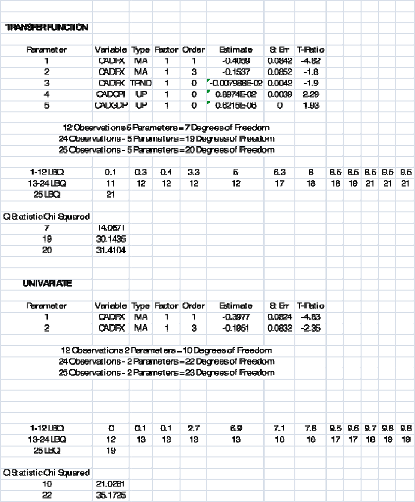
63
Table 4-2

64
Table 4-3

65
Table 4-4

Figure 3-4:
ACF and PACF for a
The diagnostic patterns of ACF and PACF for an AR model are:
ACF: declines in geometric progression from its highest value at lag 1
PACF: cuts off abruptly after lag 1
The opposite types of patterns apply to an MA proc
ACF: cuts off abruptly after lag 1
PACF: declines in geometric progression from its highest value at lag 1
66
ACF and PACF for a
MA(2) process
The diagnostic patterns of ACF and PACF for an AR model are:
ACF: declines in geometric progression from its highest value at lag 1
PACF: cuts off abruptly after lag 1
The opposite types of patterns apply to an MA proc
ess:
ACF: cuts off abruptly after lag 1
PACF: declines in geometric progression from its highest value at lag 1

67
6.0 References
Alsaleh Ahmed Ali, Mohammed. "On Forecasting Exchange Rate: A Time Series
Analysis.”
http://www.statistics.gov.uk/IAOSlondon2002/contributed_papers/downloads/CP
_Alsaleh.pdf (accessed March 16, 2009).
Andrews, Rick L. “Forecasting Performance of Structural Time Series Models.”
Journal of Business & Economic Statistics, Vol. 12, No. 1 (Jan., 1994): 129-133.
Bliemel, Friedhelm, "Theil’s Forecast Accuracy Coefficient: A Clarification." The
Journal of Marketing Research, Vol. 10, No. 4 (Nov., 1973): 444-446.
Bowerman, Bruce L. O’Connell, Richard T. Time Series Forecasting: Unified Concepts
and Computer Implementation. Boston, Massachusetts: PWS Publishers. 1987.
Calderon-Rossell, Jorge R., Ben-Horim, Moshe. “The Behavior of Foreign Exchange
Rates.” Journal of International Business Studies, Vol. 13, No. 2 (Autumn,
1982): 99-111.
Choi, In. “Testing the Random Walk Hypothesis for Real Exchange Rates.” Journal of
Applied Econometrics, Vol. 14, No. 3 (May – Jun., 1999): 293-308.
Eichengreen, Barry and Tamim Bayoumi. “Macroeconomic Adjustment Under Bretton
Woods and the Post-Bretton-Woods Float: An Impulse Response Analysis.” The
Economic Journal, Vol. 104 (1994): 813-827.
Ekern, Steinar. “Adaptive Exponential Smoothing Revisited.” The Journal of the
Operational Research Society, Vol. 32, No. 9 (Sep., 1981): 775-782.
Eun, Cheol, S., and Bruce G. Resnick. International Financial Management:. New Delhi:
McGraw Hill, 2008.
Federal Reserve Bank of St. Louis. “FRED Economic data.”
http://research.stlouisfed.org/fred2 (accessed March 11, 2009).
The Federal Reserve Board. “FRB: Speech, Bernanke—International Monetary Reform
and Capital Freedom—October 14, 2004.”
http://www.federalreserve.gov/boarddocs/speeches/2004/20041014/default.htm
(accessed March 30, 2009).
The Federal Reserve Board. "FRB: Speech, Meyer - The Future of Money and of
Monetary Policy."
http://www.federalreserve.gov/boarddocs/speeches/2001/20011205/default.htm
(accessed March 15,2010).

68
The Federal Reserve Board. Schinasi, Garry, Swamy P.A.V.B. "International Finance
Discussion Papers."
http://www.federalreserve.gov/pubs/ifdp/1987/301/default.htm. (accessed April
4, 2009).
Frenkel, Jacob A. “Flexible Exchange Rates, Prices, and the Role of ‘News’: Lessons
from the 1970s.” The Journal of Political Economy, Vol. 89, No. 4 (Aug., 1981):
665-705.
Giddy, Ian H. and Gunter Dufey. "The Random Behavior of Flexible Exchange Rates:
Implications for Forecasting." Journal of International Business Studies, no. 1
(1975): 1-32. 2003.
Gujarati, Damodar. Basic Econometrics. New Delhi: Tate McGraw-Hill Publishing
Company Limited, 2003.
Johnson, Timothy C. “Volatility, Momentum, and Time-Varying Skewness in Foreign
Exchange Returns.” Journal of Business & Economic Statistics, Vol. 20, No. 3
(July 2002): 390-411.
Kaufman, Perry J. Trading Systems and Methods. New York: John Wiley and Sons,
1998.
Krugman, Paul. International Economics: Theory and Policy. Old Tappan: Pearson
Addison Wesley, 1995.
McCracken, Michael, W. and Stephen G. Sapp. "Evaluating the Predictability of
Exchange Rates Using Long-Horizon Regressions: Mind your p’s and q’s."
Journal of Money, Credit and Banking, Vol. 37, No. 3 (June 2005): 473-494.
U.S. Census Bureau. McElroy, Tucker. "A Modified Model-based Seasonal Adjustment
that Reduces Spectral Troughs and Negative Seasonal Correlation."
http://www.census.gov/srd/www/abstract/rrs2008-12.htm (accessed March 2,
2009).
Mills, Terrence C. Time Series Techniques for Economists. New York: Cambridge
University Press, 2003.
Murphree, Eily, and Anne Koehler. "A comparison of the Akaike and Schwarz Criteria
for Selecting Model Order." Applied Statistics, No. 37 (1988): 187-195.
Mullinex, Andrew W. and Victor Murnide. Handbook of International Banking. London
Edward Elgar Publishing Limited, 2003.350-358.
Mussa, Michael. “A Model of Exchange Rate Dynamics.” The Journal of Political
Economy, Vol. 90, No. 1 (Feb., 1982): 74-104.
69
Rogoff, Kenneth and Richard Meese. "Was it Real? The Exchange Rate-Interest
Differential Relation Over the Modern Floating-Rate Period." The Journal of
Finance, No. 43 (September 1988): 933-948.
SAS Institute Inc., Forecasting Examples for Business and Economics. Cary, NC: 1996.
Sharma, J.K. Business Statistics: New Delhi, India: Dorling Kindersley, 2007.
Vandaele, Walter. Applied Time Series and Box-Jenkins Models. San Diego: Academic
Press Inc., 1983.
Wade, Robert. Governing The Market. Economic Theory and the Role of Government in
East Asian Industrialization. New Jersey: Princeton University Press, 1990. 159-
168.
Wallich, Henry C. “What Makes Exchange Rates Move?” Challenge, Vol. 20, No. 3
(Jul/Aug 1977): 34-40.
West, Kenneth D. and Charles Engel. "Accounting for Exchange-Rate Variability in
Present-Value Models When the Discount Factor Is near 1." The American
Economic Review, No. 94 (2004): 119-125.
Wolff, Christian C.P. “Time-Varying Parameters and the Out-of-Sample Forecasting
Performance of Structural Exchange Rate Models.” Journal of Business &
Economic Statistics, Vol. 5, No. 1 (January, 1987): 87-97.
Zhang, G.P., W. and V.L.Berardi. "Time Series Forecasting with Neural Network
Ensembles: An application for Exchange Rate Prediction." The Journal of the
Operational Research Society , Vol. 52, No. 6 (June, 2001): 652-664.

70
7.0 Appendix
UK Transfer Function Output
SUMMARY OF THE MODEL
OUTPUT VARIABLE -- UKFX
INPUT VARIABLES -- NOISE UKCPI UKGDP
PARAMETER VARIABLE TYPE FACTOR ORDER ESTIMATE ST. ERR. T-RATIO
1 UKFX MA 1 1 -0.3473 0.0864 -4.02
2 UKFX TRND 1 0 -0.9614E-02 0.0135 -0.71
3 UKCPI UP 1 0 -0.3193E-03 0.0103 -0.03
4 UKGDP UP 1 0 0.3512E-05 0.0000 0.76
ESTIMATION BY BACKCASTING METHOD
RELATIVE CHANGE IN RESIDUAL SUM OF SQUARES LESS THAN 0.5000E-04
SUMMARY OF THE MODEL
OUTPUT VARIABLE -- UKFX
INPUT VARIABLES -- NOISE UKCPI UKGDP
PARAMETER VARIABLE TYPE FACTOR ORDER ESTIMATE ST. ERR. T-RATIO
1 UKFX MA 1 1 -0.3471 0.0864 -4.02
2 UKFX TRND 1 0 -0.9669E-02 0.0135 -0.72
3 UKCPI UP 1 0 -0.3259E-03 0.0103 -0.03
4 UKGDP UP 1 0 0.3541E-05 0.0000 0.76
ACF Var is UKFXresidb. Maxlag is 25. lbq./
AUTOCORRELATIONS
1- 12 -.03 -.10 -.04 0.0 -.09 .12 .08 -.04 -.08 -.02 .03 .02
ST.E. .09 .09 .09 .09 .09 .09 .09 .09 .09 .09 .09 .09
L.-B. Q .10 1.4 1.5 1.5 2.5 4.4 5.2 5.3 6.3 6.3 6.4 6.5
13- 24 -.07 .11 -.01 -.25 .02 .07 .02 -.15 .13 -.04 -.19 -.03
ST.E. .09 .09 .10 .10 .10 .10 .10 .10 .10 .10 .10 .11
L.-B. Q 7.1 8.8 8.8 18. 18. 19. 19. 22. 25. 25. 30. 31.
25- 25 .04
ST.E. .11
L.-B. Q 31.
71
PLOT OF AUTOCORRELATIONS
-1.0 -0.8 -0.6 -0.4 -0.2 0.0 0.2 0.4 0.6 0.8 1.0
LAG CORR. +----+----+----+----+----+----+----+----+----+----+
I
1 -0.028 + XI +
2 -0.099 + XXI +
3 -0.037 + XI +
4 0.004 + I +
5 -0.086 + XXI +
6 0.121 + IXXX +
7 0.075 + IXX +
8 -0.036 + XI +
9 -0.082 + XXI +
10 -0.018 + I +
11 0.033 + IX +
12 0.022 + IX +
13 -0.068 + XXI +
14 0.109 + IXXX +
15 -0.008 + I +
16 -0.250 X+XXXXI +
17 0.024 + IX +
18 0.074 + IXX +
19 0.018 + I +
20 -0.148 +XXXXI +
21 0.129 + IXXX +
22 -0.040 + XI +
23 -0.192 XXXXXI +
24 -0.033 + XI +
25 0.040 + IX +
PACF Var is UKFXresidb. Maxlag is 25./
PARTIAL AUTOCORRELATIONS
1- 12 -.03 -.10 -.04 -.01 -.10 .12 .07 -.02 -.06 -.03 .04 .01
ST.E. .09 .09 .09 .09 .09 .09 .09 .09 .09 .09 .09 .09
13- 24 -.09 .10 0.0 -.23 .02 .01 .04 -.17 .09 .01 -.18 -.06
ST.E. .09 .09 .09 .09 .09 .09 .09 .09 .09 .09 .09 .09
25- 25 -.04
ST.E. .09
72
PLOT OF PARTIAL AUTOCORRELATIONS
-1.0 -0.8 -0.6 -0.4 -0.2 0.0 0.2 0.4 0.6 0.8 1.0
LAG CORR. +----+----+----+----+----+----+----+----+----+----+
I
1 -0.028 + XI +
2 -0.100 +XXXI +
3 -0.043 + XI +
4 -0.008 + I +
5 -0.095 + XXI +
6 0.115 + IXXX+
7 0.066 + IXX +
8 -0.015 + I +
9 -0.062 + XXI +
10 -0.031 + XI +
11 0.037 + IX +
12 0.013 + I +
13 -0.086 + XXI +
14 0.105 + IXXX+
15 0.002 + I +
16 -0.231 XX+XXXI +
17 0.017 + I +
18 0.011 + I +
19 0.036 + IX +
20 -0.166 XXXXI +
21 0.091 + IXX +
22 0.006 + I +
23 -0.183 X+XXXI +
24 -0.063 + XXI +
25 -0.044 + XI +
CCF Var are Rx, UKFXresidb. Maxlag is 24./
CORRELATION OF Rx AND UKFXresi IS -0.02
CROSS CORRELATIONS OF Rx (I) AND UKFXresi(I+K)
1- 12 -.06 .09 -.09 .12 .15 -.18 .03 0.0 -.08 -.11 0.0 -.06
ST.E. .09 .09 .09 .09 .09 .09 .09 .09 .10 .10 .10 .10
13- 24 -.04 .05 -.06 -.01 -.08 -.12 .01 0.0 .06 .04 .02 -.11
ST.E. .10 .10 .10 .10 .10 .10 .10 .10 .10 .10 .10 .10
CROSS CORRELATIONS OF UKFXresi(I) AND Rx (I+K)
1- 12 .06 -.01 .08 .04 -.01 .14 .03 -.02 -.22 .11 -.08 .10
ST.E. .09 .09 .09 .09 .09 .09 .09 .09 .10 .10 .10 .10
13- 24 .11 .13 0.0 -.04 .09 .08 -.01 .08 -.05 -.07 -.01 .05
ST.E. .10 .10 .10 .10 .10 .10 .10 .10 .10 .10 .10 .10
73
TRANSFER FUNCTION WEIGHTS
SCCF(X(I),Y(I+K)) SCCF(Y(I),X(I+K))
LAG *SY/SX *SX/SY *SY/SX *SX/SY
0 -0.00292 -0.08726 -0.00292 -0.08726
1 -0.01177 -0.35226 0.01044 0.31248
2 0.01729 0.51751 -0.00243 -0.07266
3 -0.01650 -0.49376 0.01494 0.44713
4 0.02141 0.64055 0.00727 0.21753
5 0.02695 0.80649 -0.00115 -0.03442
6 -0.03338 -0.99881 0.02538 0.75963
7 0.00597 0.17869 0.00608 0.18196
8 0.00079 0.02351 -0.00421 -0.12611
9 -0.01453 -0.43489 -0.04003 -1.19788
10 -0.02062 -0.61699 0.02050 0.61348
11 0.00077 0.02292 -0.01407 -0.42100
12 -0.01052 -0.31485 0.01804 0.53986
13 -0.00703 -0.21048 0.02009 0.60106
14 0.00830 0.24830 0.02301 0.68851
15 -0.01078 -0.32261 -0.00061 -0.01817
16 -0.00233 -0.06978 -0.00821 -0.24557
17 -0.01479 -0.44268 0.01651 0.49405
18 -0.02276 -0.68096 0.01478 0.44236
19 0.00112 0.03341 -0.00260 -0.07775
20 0.00020 0.00602 0.01503 0.44984
21 0.01069 0.32001 -0.00949 -0.28398
22 0.00675 0.20192 -0.01223 -0.36586
23 0.00315 0.09441 -0.00125 -0.03743
24 -0.01924 -0.57572 0.00980 0.29320
WHERE X(I) IS THE FIRST SERIES, Y(I) THE SECOND
SERIES, SX THE STANDARD ERROR OF X(I), AND SY
THE STANDARD ERROR OF Y(I)
74
PLOT OF CROSS CORRELATIONS
-1.0 -0.8 -0.6 -0.4 -0.2 0.0 0.2 0.4 0.6 0.8 1.0
LAG CORR. +----+----+----+----+----+----+----+----+----+----+
I
-24 0.054 + IX +
-23 -0.007 + I +
-22 -0.067 + XXI +
-21 -0.052 + XI +
-20 0.082 + IXX +
-19 -0.014 + I +
-18 0.081 + IXX +
-17 0.090 + IXX +
-16 -0.045 + XI +
-15 -0.003 + I +
-14 0.126 + IXXX +
-13 0.110 + IXXX +
-12 0.099 + IXX +
-11 -0.077 + XXI +
-10 0.112 + IXXX +
-9 -0.219 XXXXXI +
-8 -0.023 + XI +
-7 0.033 + IX +
-6 0.139 + IXXX +
-5 -0.006 + I +
-4 0.040 + IX +
-3 0.082 + IXX +
-2 -0.013 + I +
-1 0.057 + IX +
0 -0.016 + I +
1 -0.064 + XXI +
2 0.095 + IXX +
3 -0.090 + XXI +
4 0.117 + IXXX +
5 0.147 + IXXXX+
6 -0.183 XXXXXI +
7 0.033 + IX +
8 0.004 + I +
9 -0.079 + XXI +
10 -0.113 + XXXI +
11 0.004 + I +
12 -0.058 + XI +
13 -0.038 + XI +
14 0.045 + IX +
15 -0.059 + XI +
16 -0.013 + I +
17 -0.081 + XXI +
18 -0.124 + XXXI +
19 0.006 + I +
20 0.001 + I +
21 0.058 + IX +
22 0.037 + IX +
23 0.017 + I +
24 -0.105 + XXXI +
75
CCF Var are Rz, UKFXresidb. Maxlag is 24./
CORRELATION OF Rz AND UKFXresi IS -0.06
CROSS CORRELATIONS OF Rz (I) AND UKFXresi(I+K)
1- 12 .17 .04 .05 -.11 .07 .05 -.12 -.03 .08 .11 -.14 .11
ST.E. .09 .09 .09 .09 .09 .09 .09 .09 .09 .09 .09 .10
13- 24 0.0 -.08 .07 .02 .09 -.06 .01 .02 -.06 -.06 .17 -.09
ST.E. .10 .10 .10 .10 .10 .10 .10 .10 .10 .10 .10 .10
CROSS CORRELATIONS OF UKFXresi(I) AND Rz (I+K)
1- 12 .12 .04 -.03 .03 -.01 -.14 -.14 .18 .04 -.15 .02 .14
ST.E. .09 .09 .09 .09 .09 .09 .09 .09 .09 .09 .09 .10
13- 24 -.05 -.03 -.05 -.04 -.01 -.13 -.06 -.13 -.05 .08 -.01 -.12
ST.E. .10 .10 .10 .10 .10 .10 .10 .10 .10 .10 .10 .10
TRANSFER FUNCTION WEIGHTS
SCCF(X(I),Y(I+K)) SCCF(Y(I),X(I+K))
LAG *SY/SX *SX/SY *SY/SX *SX/SY
0 0.00000-1045.97168 0.00000-1045.97168
1 0.00001 2964.16382 0.00001 2195.97852
2 0.00000 790.36121 0.00000 781.38202
3 0.00000 848.15997 0.00000 -486.46616
4 -0.00001-1953.31458 0.00000 520.46820
5 0.00000 1278.01343 0.00000 -232.91913
6 0.00000 927.20282 -0.00001-2583.44189
7 -0.00001-2157.64502 -0.00001-2580.37134
8 0.00000 -487.15939 0.00001 3261.94067
9 0.00000 1508.58594 0.00000 702.39929
10 0.00001 1978.64709 -0.00001-2614.45215
11 -0.00001-2484.01025 0.00000 296.38187
12 0.00001 1928.05713 0.00001 2488.11011
13 0.00000 -38.79346 0.00000 -930.44269
14 0.00000-1422.75769 0.00000 -457.82623
15 0.00000 1227.00415 0.00000 -925.75903
16 0.00000 405.16898 0.00000 -662.14160
17 0.00001 1616.67615 0.00000 -219.36798
18 0.00000-1104.38452 -0.00001-2363.70068
19 0.00000 243.61572 0.00000-1159.70154
20 0.00000 431.63895 -0.00001-2369.34058
21 0.00000-1100.03650 0.00000 -953.98151
22 0.00000-1070.74438 0.00000 1359.90308
23 0.00001 3015.40332 0.00000 -181.38884
24 -0.00001-1676.61523 -0.00001-2064.61060
WHERE X(I) IS THE FIRST SERIES, Y(I) THE SECOND
SERIES, SX THE STANDARD ERROR OF X(I), AND SY
THE STANDARD ERROR OF Y(I)
76
PLOT OF CROSS CORRELATIONS
-1.0 -0.8 -0.6 -0.4 -0.2 0.0 0.2 0.4 0.6 0.8 1.0
LAG CORR. +----+----+----+----+----+----+----+----+----+----+
I
-24 -0.116 + XXXI +
-23 -0.010 + I +
-22 0.076 + IXX +
-21 -0.053 + XI +
-20 -0.133 + XXXI +
-19 -0.065 + XXI +
-18 -0.132 + XXXI +
-17 -0.012 + I +
-16 -0.037 + XI +
-15 -0.052 + XI +
-14 -0.026 + XI +
-13 -0.052 + XI +
-12 0.139 + IXXX +
-11 0.017 + I +
-10 -0.147 +XXXXI +
-9 0.039 + IX +
-8 0.183 + IXXXXX
-7 -0.145 +XXXXI +
-6 -0.145 +XXXXI +
-5 -0.013 + I +
-4 0.029 + IX +
-3 -0.027 + XI +
-2 0.044 + IX +
-1 0.123 + IXXX+
0 -0.059 + XI +
1 0.166 + IXXXX
2 0.044 + IX +
3 0.048 + IX +
4 -0.109 + XXXI +
5 0.072 + IXX +
6 0.052 + IX +
7 -0.121 + XXXI +
8 -0.027 + XI +
9 0.085 + IXX +
10 0.111 + IXXX +
11 -0.139 + XXXI +
12 0.108 + IXXX +
13 -0.002 + I +
14 -0.080 + XXI +
15 0.069 + IXX +
16 0.023 + IX +
17 0.091 + IXX +
18 -0.062 + XXI +
19 0.014 + I +
20 0.024 + IX +
21 -0.062 + XXI +
22 -0.060 + XXI +
23 0.169 + IXXXX+
24 -0.094 + XXI +
77
ARIMA VAR IS UKCPI. Dforder is 1.
Arorder is '(4)'.
Maorder is '(5)'./
THE CURRENT MODEL HAS
OUTPUT VARIABLE = UKCPI
INPUT VARIABLE = NOISE
ESTIMATION BY CONDITIONAL LEAST SQUARES METHOD
RELATIVE CHANGE IN RESIDUAL SUM OF SQUARES LESS THAN 0.5000E-04
SUMMARY OF THE MODEL
OUTPUT VARIABLE -- UKCPI
INPUT VARIABLES -- NOISE
PARAMETER VARIABLE TYPE FACTOR ORDER ESTIMATE ST. ERR. T-RATIO
1 UKCPI MA 1 5 0.1262 0.0989 1.28
2 UKCPI AR 1 4 0.8526 0.0457 18.66
Forecast Cases are 25. Join./
FORECAST ON VARIABLE UKCPI
PERIOD FORECASTS ST. ERR. ACTUAL RESIDUAL
125 116.47323 0.45107
126 117.58923 0.63790
127 117.80406 0.78127
128 118.84435 0.90213
129 119.29721 1.22968
130 120.24866 1.45550
131 120.43182 1.65071
132 121.31873 1.82515
133 121.70481 2.13439
134 122.51598 2.38223
135 122.67213 2.60661
136 123.42826 2.81315
137 123.75742 3.11493
138 124.44897 3.37384
139 124.58211 3.61425
140 125.22675 3.83963
141 125.50738 4.13489
142 126.09697 4.39827
143 126.21047 4.64675
144 126.76007 4.88261
145 126.99932 5.17086
146 127.50198 5.43454
147 127.59875 5.68601
148 128.06731 5.92682
149 128.27129 6.20749
STANDARD ERROR = 0.451065 BY CONDITIONAL METHOD
78
ARIMA VAR IS UKGDP. Dforder is 1.
Arorder is '(1)'. /
THE CURRENT MODEL HAS
OUTPUT VARIABLE = UKGDP
INPUT VARIABLE = NOISE
ESTIMATION BY CONDITIONAL LEAST SQUARES METHOD
RELATIVE CHANGE IN EACH ESTIMATE LESS THAN 0.1000E-03
SUMMARY OF THE MODEL
OUTPUT VARIABLE -- UKGDP
INPUT VARIABLES -- NOISE
PARAMETER VARIABLE TYPE FACTOR ORDER ESTIMATE ST. ERR. T-RATIO
1 UKGDP AR 1 1 0.7599 0.0585 13.00
Forecast Cases are 25. Join./
FORECAST ON VARIABLE UKGDP
PERIOD FORECASTS ST. ERR. ACTUAL RESIDUAL
125 327644.12500 1436.66895
126 326470.15600 2908.06494
127 325578.03100 4442.19971
128 324900.12500 5969.99756
129 324384.96900 7456.51367
130 323993.50000 8885.02246
131 323696.03100 10248.77540
132 323469.96900 11546.56150
133 323298.18800 12780.20020
134 323167.65600 13953.08890
135 323068.46900 15069.35550
136 322993.09400 16133.35550
137 322935.81200 17149.38870
138 322892.28100 18121.54490
139 322859.18800 19053.61720
140 322834.06200 19949.08590
141 322814.96900 20811.10350
142 322800.46900 21642.50980
143 322789.43800 22445.85350
144 322781.06200 23223.42190
145 322774.68800 23977.25590
146 322769.84400 24709.19140
147 322766.15600 25420.86130
148 322763.37500 26113.73830
149 322761.25000 26789.14060
STANDARD ERROR = 1436.67 BY CONDITIONAL METHOD
79
ARIMA VAR IS UKFX. Dforder is 1.
MAorder is '(1)'./
THE CURRENT MODEL HAS
OUTPUT VARIABLE = UKFX
INPUT VARIABLE = NOISE
ESTIMATION BY CONDITIONAL LEAST SQUARES METHOD
RELATIVE CHANGE IN EACH ESTIMATE LESS THAN 0.1000E-03
SUMMARY OF THE MODEL
OUTPUT VARIABLE -- UKFX
INPUT VARIABLES -- NOISE
PARAMETER VARIABLE TYPE FACTOR ORDER ESTIMATE ST. ERR. T-RATIO
1 UKFX MA 1 1 -0.3679 0.0841 -4.37
Forecast Cases are 25./
FORECAST ON VARIABLE UKFX
PERIOD FORECASTS ST. ERR. ACTUAL RESIDUAL
125 1.58113 0.07754
126 1.58113 0.13139
127 1.58113 0.16887
128 1.58113 0.19942
129 1.58113 0.22587
130 1.58113 0.24954
131 1.58113 0.27115
132 1.58113 0.29116
133 1.58113 0.30988
134 1.58113 0.32753
135 1.58113 0.34428
136 1.58113 0.36025
137 1.58113 0.37554
138 1.58113 0.39023
139 1.58113 0.40439
140 1.58113 0.41807
141 1.58113 0.43132
142 1.58113 0.44417
143 1.58113 0.45666
144 1.58113 0.46882
145 1.58113 0.48067
146 1.58113 0.49223
147 1.58113 0.50353
148 1.58113 0.51458
149 1.58113 0.52540
STANDARD ERROR = 0.775418E-01 BY CONDITIONAL METHOD
ESTIMATION BY CONDITIONAL LEAST SQUARES METHOD
RELATIVE CHANGE IN RESIDUAL SUM OF SQUARES LESS THAN 0.5000E-04
80
SUMMARY OF THE MODEL
OUTPUT VARIABLE -- UKFX
INPUT VARIABLES -- NOISE UKCPI UKGDP
PARAMETER VARIABLE TYPE FACTOR ORDER ESTIMATE ST. ERR. T-RATIO
1 UKFX MA 1 1 -0.3473 0.0864 -4.02
2 UKFX TRND 1 0 -0.9614E-02 0.0135 -0.71
3 UKCPI UP 1 0 -0.3193E-03 0.0103 -0.03
4 UKGDP UP 1 0 0.3512E-05 0.0000 0.76
Forecast Cases are 25./
FORECAST ON VARIABLE UKFX
PERIOD FORECASTS ST. ERR. ACTUAL RESIDUAL
125 1.57205 0.07822
126 1.55796 0.13124
127 1.54515 0.16831
128 1.53282 0.19858
129 1.52125 0.22481
130 1.50996 0.24828
131 1.49924 0.26972
132 1.48855 0.28958
133 1.47821 0.30816
134 1.46788 0.32568
135 1.45787 0.34230
136 1.44775 0.35816
137 1.43783 0.37334
138 1.42784 0.38793
139 1.41807 0.40199
140 1.40816 0.41557
141 1.39839 0.42872
142 1.38854 0.44148
143 1.37885 0.45389
144 1.36903 0.46596
145 1.35932 0.47773
146 1.34953 0.48921
147 1.33987 0.50043
148 1.33010 0.51141
149 1.32041 0.52215
STANDARD ERROR = 0.782195E-01 BY CONDITIONAL METHOD
BMDP2T - BOX-JENKINS TIME SERIES ANALYSIS
Copyright 1977, 1979, 1981, 1982, 1983, 1985, 1987, 1988, 1990, 1993
by BMDP Statistical Software, Inc.
Statistical Solutions Ltd. | Statistical Solutions
Unit 1A, South Ring Business Park | Stonehill Corporate Center, Suite 104
Kinsale Road, Cork, Ireland | 999 Broadway, Saugus, MA 01906, USA
Phone: + 353 21 4319629 | Phone: 781.231.7680
Fax: + 353 21 4319630 | Fax: 781.231.7684
e-mail: sales@statsol.ie | e-mail: i[email protected]
Website: http://www.statsol.ie | Website: http://www.statsolusa.com
Release: 8.1 (Windows 9x, 2000, Me, Xp) Date: 10/20/12 at 13:25:28
Manual: BMDP Manual Volumes 1, 2, and 3.
81
Digest: BMDP User's Digest.
IBM PC: BMDP PC Supplement -- Installation and Special Features.
JPY Transfer Function Output
SUMMARY OF THE MODEL
OUTPUT VARIABLE -- JPYFX
INPUT VARIABLES -- NOISE JPYCPI JPYGDP
PARAMETER VARIABLE TYPE FACTOR ORDER ESTIMATE ST. ERR. T-RATIO
1 JPYFX MA 1 1 -0.5497 0.0808 -6.81
2 JPYFX TRND 1 0 -1.629 1.1184 -1.46
3 JPYCPI UP 1 0 -1.607 0.7302 -2.20
4 JPYGDP UP 1 0 0.3078E-03 0.0002 2.05
ESTIMATION BY BACKCASTING METHOD
RELATIVE CHANGE IN RESIDUAL SUM OF SQUARES LESS THAN 0.5000E-04
SUMMARY OF THE MODEL
PARAMETER VARIABLE TYPE FACTOR ORDER ESTIMATE ST. ERR. T-RATIO
1 JPYFX MA 1 1 -0.5507 0.0804 -6.85
2 JPYFX TRND 1 0 -1.628 1.1212 -1.45
3 JPYCPI UP 1 0 -1.607 0.7336 -2.19
4 JPYGDP UP 1 0 0.3081E-03 0.0002 2.05
ACF Var is JPYFXresidb. Maxlag is 25. lbq./
AUTOCORRELATIONS
1- 12 -.07 -.05 .13 .01 .03 -.16 -.02 .01 -.02 .07 .04 -.01
ST.E. .09 .09 .09 .10 .10 .10 .10 .10 .10 .10 .10 .10
L.-B. Q .60 .90 2.8 2.8 3.0 6.0 6.1 6.1 6.2 6.8 7.0 7.1
13- 24 -.19 .09 -.13 -.13 .04 -.13 .10 0.0 .02 .05 -.03 -.03
ST.E. .10 .10 .10 .10 .11 .11 .11 .11 .11 .11 .11 .11
L.-B. Q 12. 13. 16. 18. 18. 20. 22. 22. 22. 22. 22. 22.
25- 25 .02
ST.E. .11
L.-B. Q 22.
82
PLOT OF AUTOCORRELATIONS
-1.0 -0.8 -0.6 -0.4 -0.2 0.0 0.2 0.4 0.6 0.8 1.0
LAG CORR. +----+----+----+----+----+----+----+----+----+----+
I
1 -0.073 + XXI +
2 -0.048 + XI +
3 0.126 + IXXX +
4 0.014 + I +
5 0.029 + IX +
6 -0.158 +XXXXI +
7 -0.015 + I +
8 0.014 + I +
9 -0.025 + XI +
10 0.071 + IXX +
11 0.041 + IX +
12 -0.011 + I +
13 -0.193 XXXXXI +
14 0.095 + IXX +
15 -0.131 + XXXI +
16 -0.125 + XXXI +
17 0.041 + IX +
18 -0.129 + XXXI +
19 0.102 + IXXX +
20 -0.003 + I +
21 0.022 + IX +
22 0.049 + IX +
23 -0.025 + XI +
24 -0.034 + XI +
25 0.018 + I +
PACF Var is JPYFXresidb. Maxlag is 25./
PARTIAL AUTOCORRELATIONS
1- 12 -.07 -.05 .12 .03 .04 -.17 -.04 -.01 .02 .09 .07 -.02
ST.E. .09 .09 .09 .09 .09 .09 .09 .09 .09 .09 .09 .09
13- 24 -.24 .04 -.15 -.05 .04 -.09 .06 0.0 .02 -.02 .03 -.09
ST.E. .09 .09 .09 .09 .09 .09 .09 .09 .09 .09 .09 .09
25- 25 .03
ST.E. .09
83
PLOT OF PARTIAL AUTOCORRELATIONS
-1.0 -0.8 -0.6 -0.4 -0.2 0.0 0.2 0.4 0.6 0.8 1.0
LAG CORR. +----+----+----+----+----+----+----+----+----+----+
I
1 -0.073 + XXI +
2 -0.054 + XI +
3 0.120 + IXXX +
4 0.030 + IX +
5 0.045 + IX +
6 -0.170 +XXXXI +
7 -0.043 + XI +
8 -0.015 + I +
9 0.017 + I +
10 0.090 + IXX +
11 0.068 + IXX +
12 -0.022 + XI +
13 -0.242 X+XXXXI +
14 0.042 + IX +
15 -0.155 +XXXXI +
16 -0.054 + XI +
17 0.041 + IX +
18 -0.094 + XXI +
19 0.059 + IX +
20 -0.004 + I +
21 0.021 + IX +
22 -0.016 + I +
23 0.026 + IX +
24 -0.087 + XXI +
25 0.034 + IX +
CCF Var are Rx, JPYFXresidb. Maxlag is 24./
CORRELATION OF Rx AND JPYFXres IS 0.02
CROSS CORRELATIONS OF Rx (I) AND JPYFXres(I+K)
1- 12 -.03 .07 .11 0.0 -.04 -.13 .05 .01 -.03 -.08 .01 -.05
ST.E. .10 .10 .10 .10 .10 .10 .10 .10 .10 .10 .10 .10
13- 24 -.12 -.02 .06 -.05 .07 .02 .12 -.03 -.04 .08 -.08 .05
ST.E. .10 .10 .10 .10 .10 .10 .10 .10 .11 .11 .11 .11
CROSS CORRELATIONS OF JPYFXres(I) AND Rx (I+K)
1- 12 0.0 .04 .11 -.06 .06 -.14 .03 -.02 -.14 .06 .04 -.24
ST.E. .10 .10 .10 .10 .10 .10 .10 .10 .10 .10 .10 .10
13- 24 .15 -.21 -.12 .07 -.06 -.14 0.0 .04 -.02 -.04 -.04 .02
ST.E. .10 .10 .10 .10 .10 .10 .10 .10 .11 .11 .11 .11
84
TRANSFER FUNCTION WEIGHTS
SCCF(X(I),Y(I+K)) SCCF(Y(I),X(I+K))
LAG *SY/SX *SX/SY *SY/SX *SX/SY
0 0.32712 0.00129 0.32712 0.00129
1 -0.45519 -0.00179 0.04122 0.00016
2 1.06297 0.00418 0.68518 0.00269
3 1.80648 0.00710 1.75597 0.00690
4 0.06132 0.00024 -0.92917 -0.00365
5 -0.60187 -0.00236 0.92852 0.00365
6 -2.01049 -0.00790 -2.18333 -0.00858
7 0.73064 0.00287 0.41595 0.00163
8 0.12123 0.00048 -0.25807 -0.00101
9 -0.42877 -0.00168 -2.17425 -0.00854
10 -1.31059 -0.00515 0.91730 0.00360
11 0.19535 0.00077 0.61070 0.00240
12 -0.82290 -0.00323 -3.74991 -0.01473
13 -1.89470 -0.00744 2.42988 0.00955
14 -0.39404 -0.00155 -3.41082 -0.01340
15 0.90936 0.00357 -1.83708 -0.00722
16 -0.80811 -0.00317 1.09116 0.00429
17 1.12752 0.00443 -0.89791 -0.00353
18 0.33669 0.00132 -2.20531 -0.00866
19 1.92400 0.00756 -0.05447 -0.00021
20 -0.42394 -0.00167 0.68925 0.00271
21 -0.68885 -0.00271 -0.36278 -0.00143
22 1.29024 0.00507 -0.68394 -0.00269
23 -1.29312 -0.00508 -0.57641 -0.00226
24 0.73830 0.00290 0.39286 0.00154
WHERE X(I) IS THE FIRST SERIES, Y(I) THE SECOND
SERIES, SX THE STANDARD ERROR OF X(I), AND SY
THE STANDARD ERROR OF Y(I)
85
PLOT OF CROSS CORRELATIONS
-1.0 -0.8 -0.6 -0.4 -0.2 0.0 0.2 0.4 0.6 0.8 1.0
LAG CORR. +----+----+----+----+----+----+----+----+----+----+
I
-24 0.025 + IX +
-23 -0.036 + XI +
-22 -0.043 + XI +
-21 -0.023 + XI +
-20 0.043 + IX +
-19 -0.003 + I +
-18 -0.138 + XXXI +
-17 -0.056 + XI +
-16 0.068 + IXX +
-15 -0.115 + XXXI +
-14 -0.214 XXXXXI +
-13 0.152 + IXXXX+
-12 -0.235 X+XXXXI +
-11 0.038 + IX +
-10 0.057 + IX +
-9 -0.136 + XXXI +
-8 -0.016 + I +
-7 0.026 + IX +
-6 -0.137 + XXXI +
-5 0.058 + IX +
-4 -0.058 + XI +
-3 0.110 + IXXX +
-2 0.043 + IX +
-1 0.003 + I +
0 0.021 + IX +
1 -0.029 + XI +
2 0.067 + IXX +
3 0.113 + IXXX +
4 0.004 + I +
5 -0.038 + XI +
6 -0.126 + XXXI +
7 0.046 + IX +
8 0.008 + I +
9 -0.027 + XI +
10 -0.082 + XXI +
11 0.012 + I +
12 -0.052 + XI +
13 -0.119 + XXXI +
14 -0.025 + XI +
15 0.057 + IX +
16 -0.051 + XI +
17 0.071 + IXX +
18 0.021 + IX +
19 0.121 + IXXX +
20 -0.027 + XI +
21 -0.043 + XI +
22 0.081 + IXX +
23 -0.081 + XXI +
24 0.046 + IX +
86
CCF Var are Rz, JPYFXresidb. Maxlag is 24./
CORRELATION OF Rz AND JPYFXres IS -0.04
CROSS CORRELATIONS OF Rz (I) AND JPYFXres(I+K)
1- 12 -.07 .04 -.04 -.07 .05 .08 .05 -.03 .02 .03 -.12 -.08
ST.E. .09 .10 .10 .10 .10 .10 .10 .10 .10 .10 .10 .10
13- 24 .07 -.11 -.10 .01 .01 -.01 .01 .02 -.02 -.09 .08 .08
ST.E. .10 .10 .10 .10 .10 .10 .10 .10 .10 .11 .11 .11
CROSS CORRELATIONS OF JPYFXres(I) AND Rz (I+K)
1- 12 -.11 .11 .01 -.01 -.04 -.16 -.06 -.09 .04 -.16 .06 .19
ST.E. .09 .10 .10 .10 .10 .10 .10 .10 .10 .10 .10 .10
13- 24 -.17 -.02 -.08 0.0 -.05 0.0 -.06 -.03 .21 .05 .09 -.07
ST.E. .10 .10 .10 .10 .10 .10 .10 .10 .10 .11 .11 .11
TRANSFER FUNCTION WEIGHTS
SCCF(X(I),Y(I+K)) SCCF(Y(I),X(I+K))
LAG *SY/SX *SX/SY *SY/SX *SX/SY
0 -0.00007 -23.96902 -0.00007 -23.96902
1 -0.00013 -41.32352 -0.00019 -62.14023
2 0.00007 22.62374 0.00020 65.91998
3 -0.00006 -20.98981 0.00002 7.08367
4 -0.00012 -40.16748 -0.00001 -4.13804
5 0.00008 27.02754 -0.00006 -20.86771
6 0.00014 44.56573 -0.00028 -93.08356
7 0.00008 26.07324 -0.00011 -35.79874
8 -0.00005 -18.10973 -0.00016 -54.01652
9 0.00004 13.75161 0.00008 24.73916
10 0.00006 18.87581 -0.00028 -91.66356
11 -0.00021 -67.80497 0.00010 32.11078
12 -0.00013 -44.41050 0.00033 108.56485
13 0.00012 39.79807 -0.00029 -95.37443
14 -0.00020 -65.31018 -0.00004 -13.04819
15 -0.00017 -56.27103 -0.00014 -46.45267
16 0.00001 4.70671 0.00001 2.66644
17 0.00002 8.07820 -0.00009 -29.41980
18 -0.00002 -5.45219 0.00000 -0.36783
19 0.00001 3.37085 -0.00011 -36.15593
20 0.00004 12.15178 -0.00005 -17.41155
21 -0.00003 -10.79318 0.00036 118.65149
22 -0.00015 -49.00639 0.00009 28.47079
23 0.00013 43.53536 0.00015 50.03826
24 0.00013 43.28736 -0.00013 -41.71620
WHERE X(I) IS THE FIRST SERIES, Y(I) THE SECOND
SERIES, SX THE STANDARD ERROR OF X(I), AND SY
THE STANDARD ERROR OF Y(I)
87
PLOT OF CROSS CORRELATIONS
-1.0 -0.8 -0.6 -0.4 -0.2 0.0 0.2 0.4 0.6 0.8 1.0
LAG CORR. +----+----+----+----+----+----+----+----+----+----+
I
-24 -0.073 + XXI +
-23 0.087 + IXX +
-22 0.050 + IX +
-21 0.207 + IXXXXX
-20 -0.030 + XI +
-19 -0.063 + XXI +
-18 -0.001 + I +
-17 -0.051 + XI +
-16 0.005 + I +
-15 -0.081 + XXI +
-14 -0.023 + XI +
-13 -0.166 +XXXXI +
-12 0.189 + IXXXXX
-11 0.056 + IX +
-10 -0.160 +XXXXI +
-9 0.043 + IX +
-8 -0.094 + XXI +
-7 -0.062 + XXI +
-6 -0.162 +XXXXI +
-5 -0.036 + XI +
-4 -0.007 + I +
-3 0.012 + I +
-2 0.115 + IXXX +
-1 -0.108 + XXXI +
0 -0.042 + XI +
1 -0.072 + XXI +
2 0.039 + IX +
3 -0.037 + XI +
4 -0.070 + XXI +
5 0.047 + IX +
6 0.078 + IXX +
7 0.045 + IX +
8 -0.032 + XI +
9 0.024 + IX +
10 0.033 + IX +
11 -0.118 + XXXI +
12 -0.077 + XXI +
13 0.069 + IXX +
14 -0.114 + XXXI +
15 -0.098 + XXI +
16 0.008 + I +
17 0.014 + I +
18 -0.009 + I +
19 0.006 + I +
20 0.021 + IX +
21 -0.019 + I +
22 -0.085 + XXI +
23 0.076 + IXX +
24 0.075 + IXX +
88
ARIMA VAR IS JPYCPI. Dforder is 1.
Arorder is '(4)'.
Maorder is '(2,3,5)'./
THE CURRENT MODEL HAS
OUTPUT VARIABLE = JPYCPI
INPUT VARIABLE = NOISE
ESTIMATION BY CONDITIONAL LEAST SQUARES METHOD
RELATIVE CHANGE IN RESIDUAL SUM OF SQUARES LESS THAN 0.5000E-04
SUMMARY OF THE MODEL
OUTPUT VARIABLE -- JPYCPI
INPUT VARIABLES -- NOISE
PARAMETER VARIABLE TYPE FACTOR ORDER ESTIMATE ST. ERR. T-RATIO
1 JPYCPI MA 1 2 -0.2311 0.0986 -2.34
2 JPYCPI MA 1 3 -0.9222E-01 0.1018 -0.91
3 JPYCPI MA 1 5 -0.3505E-01 0.1033 -0.34
4 JPYCPI AR 1 4 0.5931 0.0738 8.04
Forecast Cases are 25. Join./
FORECAST ON VARIABLE JPYCPI
PERIOD FORECASTS ST. ERR. ACTUAL RESIDUAL
125 102.03491 0.46268
126 102.37516 0.65433
127 102.88356 0.86751
128 102.47814 1.06181
129 102.54932 1.38333
130 102.75111 1.65190
131 103.05262 1.91376
132 102.81218 2.15539
133 102.85439 2.44503
134 102.97407 2.70794
135 103.15289 2.96254
136 103.01029 3.20260
137 103.03532 3.46133
138 103.10630 3.70405
139 103.21236 3.93935
140 103.12778 4.16424
141 103.14263 4.39558
142 103.18472 4.61638
143 103.24762 4.83097
144 103.19746 5.03791
145 103.20627 5.24606
146 103.23123 5.44679
147 103.26853 5.64242
148 103.23878 5.83229
149 103.24401 6.02114
STANDARD ERROR = 0.462682 BY CONDITIONAL METHOD
89
ARIMA VAR IS JPYGDP. Dforder is 1.
Arorder is '(1,2,3)'./
THE CURRENT MODEL HAS
OUTPUT VARIABLE = JPYGDP
INPUT VARIABLE = NOISE
ESTIMATION BY CONDITIONAL LEAST SQUARES METHOD
RELATIVE CHANGE IN EACH ESTIMATE LESS THAN 0.1000E-03
SUMMARY OF THE MODEL
OUTPUT VARIABLE -- JPYGDP
INPUT VARIABLES -- NOISE
PARAMETER VARIABLE TYPE FACTOR ORDER ESTIMATE ST. ERR. T-RATIO
1 JPYGDP AR 1 1 0.2204 0.0950 2.32
2 JPYGDP AR 1 2 0.1731 0.0956 1.81
3 JPYGDP AR 1 3 0.3292 0.0948 3.47
Forecast Cases are 25. Join./
FORECAST ON VARIABLE JPYGDP
PERIOD FORECASTS ST. ERR. ACTUAL RESIDUAL
125 531094.62500 4245.46631
126 524555.50000 6698.43457
127 516342.25000 9074.92871
128 511322.84400 12024.95700
129 506641.90600 14871.55270
130 502037.43800 17676.85550
131 498559.78100 20541.68750
132 495455.15600 23342.54490
133 492653.00000 26086.61130
134 490353.03100 28788.51370
135 488338.93800 31423.25000
136 486574.37500 33992.31250
137 485079.59400 36498.65620
138 483781.59400 38938.22270
139 482655.81200 41312.77730
140 481690.87500 43624.45700
141 480856.00000 45874.19920
142 480134.34400 48064.27340
143 479513.09400 50197.01950
144 478976.37500 52274.56250
145 478512.93800 54299.28130
146 478113.34400 56273.51560
147 477768.34400 58199.52340
148 477470.56200 60079.53520
149 477213.65600 61915.70700
STANDARD ERROR = 4245.47 BY CONDITIONAL METHOD
90
ARIMA VAR IS JPYFX. Dforder is 1.
MAorder is '(1)'./
THE CURRENT MODEL HAS
OUTPUT VARIABLE = JPYFX
INPUT VARIABLE = NOISE
ESTIMATION BY CONDITIONAL LEAST SQUARES METHOD
RELATIVE CHANGE IN RESIDUAL SUM OF SQUARES LESS THAN 0.5000E-04
SUMMARY OF THE MODEL
OUTPUT VARIABLE -- JPYFX
INPUT VARIABLES -- NOISE
PARAMETER VARIABLE TYPE FACTOR ORDER ESTIMATE ST. ERR. T-RATIO
1 JPYFX MA 1 1 -0.4188 0.0859 -4.87
Forecast Cases are 25./
FORECAST ON VARIABLE JPYFX
PERIOD FORECASTS ST. ERR. ACTUAL RESIDUAL
125 90.88712 7.52841
126 90.88712 13.06772
127 90.88712 16.87760
128 90.88712 19.97352
129 90.88712 22.65016
130 90.88712 25.04232
131 90.88712 27.22510
132 90.88712 29.24541
133 90.88712 31.13490
134 90.88712 32.91611
135 90.88712 34.60576
136 90.88712 36.21666
137 90.88712 37.75891
138 90.88712 39.24058
139 90.88712 40.66831
140 90.88712 42.04758
141 90.88712 43.38303
142 90.88712 44.67858
143 90.88712 45.93761
144 90.88712 47.16304
145 90.88712 48.35742
146 90.88712 49.52301
147 90.88712 50.66179
148 90.88712 51.77552
149 90.88712 52.86580
STANDARD ERROR = 7.52841 BY CONDITIONAL METHOD
91
SUMMARY OF THE MODEL
OUTPUT VARIABLE -- JPYFX
INPUT VARIABLES -- NOISE JPYCPI JPYGDP
PARAMETER VARIABLE TYPE FACTOR ORDER ESTIMATE ST. ERR. T-RATIO
1 JPYFX MA 1 1 -0.5497 0.0808 -6.81
2 JPYFX TRND 1 0 -1.629 1.1184 -1.46
3 JPYCPI UP 1 0 -1.607 0.7302 -2.20
4 JPYGDP UP 1 0 0.3078E-03 0.0002 2.05
Forecast Cases are 25./
FORECAST ON VARIABLE JPYFX
PERIOD FORECASTS ST. ERR. ACTUAL RESIDUAL
125 87.71048 7.33469
126 83.52147 13.52783
127 78.54692 17.66937
128 76.02389 21.00978
129 72.83924 23.88756
130 69.46825 26.45411
131 66.28389 28.79279
132 64.08519 30.95527
133 61.52542 32.97626
134 58.99577 34.88034
135 56.45908 36.68573
136 54.51568 38.40634
137 52.38596 40.05311
138 50.24300 41.63479
139 48.09668 43.15855
140 46.30619 44.63031
141 44.39598 46.05507
142 42.47684 47.43705
143 40.55519 48.77990
144 38.84121 50.08675
145 37.05505 51.36037
146 35.26258 52.60315
147 33.46709 53.81725
148 31.79387 55.00455
149 30.07703 56.16676
STANDARD ERROR = 7.33469 BY CONDITIONAL METHOD
BMDP2T - BOX-JENKINS TIME SERIES ANALYSIS
Copyright 1977, 1979, 1981, 1982, 1983, 1985, 1987, 1988, 1990, 1993
by BMDP Statistical Software, Inc.
Statistical Solutions Ltd. | Statistical Solutions
Unit 1A, South Ring Business Park | Stonehill Corporate Center, Suite 104
Kinsale Road, Cork, Ireland | 999 Broadway, Saugus, MA 01906, USA
Phone: + 353 21 4319629 | Phone: 781.231.7680
Fax: + 353 21 4319630 | Fax: 781.231.7684
e-mail: sales@statsol.ie | e-mail: info@statsolusa.com
Website: http://www.statsol.ie | Website: http://www.statsolusa.com
Release: 8.1 (Windows 9x, 2000, Me, Xp) Date: 07/11/12 at 18:52:30
Manual: BMDP Manual Volumes 1, 2, and 3.
Digest: BMDP User's Digest.
92
IBM PC: BMDP PC Supplement -- Installation and Special Features.
CAD Transfer Function Output
SUMMARY OF THE MODEL
OUTPUT VARIABLE -- CADFX
INPUT VARIABLES -- NOISE CADCPI CADGDP
PARAMETER VARIABLE TYPE FACTOR ORDER ESTIMATE ST. ERR. T-RATIO
1 CADFX MA 1 1 -0.4039 0.0844 -4.78
2 CADFX MA 1 3 -0.1518 0.0856 -1.77
3 CADFX TRND 1 0 -0.8067E-02 0.0042 -1.93
4 CADCPI UP 1 0 0.8966E-02 0.0039 2.29
5 CADGDP UP 1 0 0.6268E-06 0.0000 1.94
ESTIMATION BY BACKCASTING METHOD
RELATIVE CHANGE IN RESIDUAL SUM OF SQUARES LESS THAN 0.5000E-04
SUMMARY OF THE MODEL
OUTPUT VARIABLE -- CADFX
INPUT VARIABLES -- NOISE CADCPI CADGDP
PARAMETER VARIABLE TYPE FACTOR ORDER ESTIMATE ST. ERR. T-RATIO
1 CADFX MA 1 1 -0.4059 0.0842 -4.82
2 CADFX MA 1 3 -0.1537 0.0852 -1.80
3 CADFX TRND 1 0 -0.7988E-02 0.0042 -1.90
4 CADCPI UP 1 0 0.8974E-02 0.0039 2.29
5 CADGDP UP 1 0 0.6215E-06 0.0000 1.93
ACF Var is CADFXresidb. Maxlag is 25. lbq./
AUTOCORRELATIONS
1- 12 -.02 -.04 -.04 -.15 -.11 .10 .11 .06 .01 -.02 .08 .01
ST.E. .09 .09 .09 .09 .09 .09 .09 .10 .10 .10 .10 .10
L.-B. Q .10 .30 .40 3.3 5.0 6.3 8.0 8.5 8.5 8.5 9.5 9.5
13- 24 -.10 .07 -.05 .01 .02 .18 -.08 -.07 -.06 -.10 .01 .01
ST.E. .10 .10 .10 .10 .10 .10 .10 .10 .10 .10 .10 .10
L.-B. Q 11. 12. 12. 12. 12. 17. 18. 18. 19. 21. 21. 21.
25- 25 .01
ST.E. .10
L.-B. Q 21.
93
PLOT OF AUTOCORRELATIONS
-1.0 -0.8 -0.6 -0.4 -0.2 0.0 0.2 0.4 0.6 0.8 1.0
LAG CORR. +----+----+----+----+----+----+----+----+----+----+
I
1 -0.024 + XI +
2 -0.041 + XI +
3 -0.036 + XI +
4 -0.149 XXXXI +
5 -0.112 + XXXI +
6 0.101 + IXXX +
7 0.113 + IXXX +
8 0.057 + IX +
9 0.009 + I +
10 -0.016 + I +
11 0.084 + IXX +
12 0.011 + I +
13 -0.100 + XXXI +
14 0.074 + IXX +
15 -0.051 + XI +
16 0.005 + I +
17 0.019 + I +
18 0.178 + IXXXX+
19 -0.077 + XXI +
20 -0.067 + XXI +
21 -0.061 + XXI +
22 -0.105 + XXXI +
23 0.008 + I +
24 0.006 + I +
25 0.009 + I +
PACF Var is CADFXresidb. Maxlag is 25./
PARTIAL AUTOCORRELATIONS
1- 12 -.02 -.04 -.04 -.15 -.13 .08 .10 .04 -.01 .01 .15 .06
ST.E. .09 .09 .09 .09 .09 .09 .09 .09 .09 .09 .09 .09
13- 24 -.11 .05 -.03 .04 -.03 .15 -.06 -.07 -.06 -.09 0.0 -.06
ST.E. .09 .09 .09 .09 .09 .09 .09 .09 .09 .09 .09 .09
25- 25 -.07
ST.E. .09
94
PLOT OF PARTIAL AUTOCORRELATIONS
-1.0 -0.8 -0.6 -0.4 -0.2 0.0 0.2 0.4 0.6 0.8 1.0
LAG CORR. +----+----+----+----+----+----+----+----+----+----+
I
1 -0.024 + XI +
2 -0.041 + XI +
3 -0.038 + XI +
4 -0.153 XXXXI +
5 -0.128 +XXXI +
6 0.080 + IXX +
7 0.103 + IXXX+
8 0.044 + IX +
9 -0.007 + I +
10 0.008 + I +
11 0.149 + IXXXX
12 0.059 + IX +
13 -0.107 +XXXI +
14 0.052 + IX +
15 -0.027 + XI +
16 0.036 + IX +
17 -0.028 + XI +
18 0.151 + IXXXX
19 -0.064 + XXI +
20 -0.069 + XXI +
21 -0.063 + XXI +
22 -0.088 + XXI +
23 0.004 + I +
24 -0.062 + XXI +
25 -0.074 + XXI +
CCF Var are Rx, CADFXresidb. Maxlag is 24./
CORRELATION OF Rx AND CADFXres IS 0.07
CROSS CORRELATIONS OF Rx (I) AND CADFXres(I+K)
1- 12 .02 -.06 .12 -.05 -.03 -.11 .01 .15 .04 -.02 -.12 .03
ST.E. .09 .09 .09 .09 .09 .09 .09 .09 .10 .10 .10 .10
13- 24 -.08 .03 -.05 -.09 .05 -.03 .13 .06 .13 -.03 -.22 -.13
ST.E. .10 .10 .10 .10 .10 .10 .10 .10 .10 .10 .10 .10
CROSS CORRELATIONS OF CADFXres(I) AND Rx (I+K)
1- 12 -.11 .11 .26 .05 -.09 0.0 -.12 -.06 .01 .08 .01 -.03
ST.E. .09 .09 .09 .09 .09 .09 .09 .09 .10 .10 .10 .10
13- 24 -.05 0.0 .09 -.01 -.18 .03 .05 -.04 .04 -.04 -.14 -.05
ST.E. .10 .10 .10 .10 .10 .10 .10 .10 .10 .10 .10 .10
95
TRANSFER FUNCTION WEIGHTS
SCCF(X(I),Y(I+K)) SCCF(Y(I),X(I+K))
LAG *SY/SX *SX/SY *SY/SX *SX/SY
0 0.00280 1.54633 0.00280 1.54633
1 0.00079 0.43473 -0.00456 -2.51905
2 -0.00270 -1.49456 0.00488 2.69772
3 0.00520 2.87761 0.01097 6.06684
4 -0.00211 -1.16475 0.00209 1.15322
5 -0.00147 -0.81035 -0.00371 -2.05311
6 -0.00466 -2.57445 0.00002 0.01004
7 0.00062 0.34156 -0.00511 -2.82806
8 0.00629 3.47921 -0.00235 -1.30210
9 0.00159 0.88002 0.00036 0.19727
10 -0.00087 -0.48367 0.00332 1.83550
11 -0.00503 -2.78003 0.00053 0.29094
12 0.00132 0.72857 -0.00133 -0.73640
13 -0.00334 -1.84591 -0.00193 -1.06796
14 0.00120 0.66484 -0.00003 -0.01558
15 -0.00219 -1.20927 0.00387 2.13932
16 -0.00392 -2.16985 -0.00031 -0.17165
17 0.00212 1.17258 -0.00754 -4.17040
18 -0.00108 -0.59682 0.00122 0.67649
19 0.00561 3.09983 0.00224 1.23798
20 0.00248 1.37044 -0.00173 -0.95485
21 0.00547 3.02730 0.00153 0.84876
22 -0.00116 -0.64140 -0.00177 -0.97698
23 -0.00953 -5.26942 -0.00596 -3.29873
24 -0.00559 -3.09005 -0.00205 -1.13317
WHERE X(I) IS THE FIRST SERIES, Y(I) THE SECOND
SERIES, SX THE STANDARD ERROR OF X(I), AND SY
THE STANDARD ERROR OF Y(I)
96
PLOT OF CROSS CORRELATIONS
-1.0 -0.8 -0.6 -0.4 -0.2 0.0 0.2 0.4 0.6 0.8 1.0
LAG CORR. +----+----+----+----+----+----+----+----+----+----+
I
-24 -0.048 + XI +
-23 -0.140 +XXXXI +
-22 -0.042 + XI +
-21 0.036 + IX +
-20 -0.041 + XI +
-19 0.053 + IX +
-18 0.029 + IX +
-17 -0.177 +XXXXI +
-16 -0.007 + I +
-15 0.091 + IXX +
-14 -0.001 + I +
-13 -0.045 + XI +
-12 -0.031 + XI +
-11 0.012 + I +
-10 0.078 + IXX +
-9 0.008 + I +
-8 -0.055 + XI +
-7 -0.120 + XXXI +
-6 0.000 + I +
-5 -0.087 + XXI +
-4 0.049 + IX +
-3 0.258 + IXXXX+X
-2 0.115 + IXXX +
-1 -0.107 + XXXI +
0 0.066 + IXX +
1 0.018 + I +
2 -0.064 + XXI +
3 0.122 + IXXX +
4 -0.050 + XI +
5 -0.034 + XI +
6 -0.109 + XXXI +
7 0.015 + I +
8 0.148 + IXXXX+
9 0.037 + IX +
10 -0.021 + XI +
11 -0.118 + XXXI +
12 0.031 + IX +
13 -0.078 + XXI +
14 0.028 + IX +
15 -0.051 + XI +
16 -0.092 + XXI +
17 0.050 + IX +
18 -0.025 + XI +
19 0.132 + IXXX +
20 0.058 + IX +
21 0.129 + IXXX +
22 -0.027 + XI +
23 -0.224 X+XXXXI +
24 -0.131 + XXXI +
97
CCF Var are Rz, CADFXresidb. Maxlag is 24./
CORRELATION OF Rz AND CADFXres IS 0.01
CROSS CORRELATIONS OF Rz (I) AND CADFXres(I+K)
1- 12 -.10 .05 .02 -.14 -.04 -.11 .12 .06 .04 .07 .03 0.0
ST.E. .09 .09 .09 .09 .09 .09 .09 .09 .09 .09 .09 .09
13- 24 .04 .07 .08 .04 .01 -.09 .10 -.07 .06 .08 .07 .05
ST.E. .10 .10 .10 .10 .10 .10 .10 .10 .10 .10 .10 .10
CROSS CORRELATIONS OF CADFXres(I) AND Rz (I+K)
1- 12 .13 .13 0.0 .02 -.16 -.13 -.13 .09 .08 -.08 0.0 -.12
ST.E. .09 .09 .09 .09 .09 .09 .09 .09 .09 .09 .09 .09
13- 24 -.03 -.03 .07 -.09 -.08 -.01 -.03 .03 0.0 -.11 -.13 .02
ST.E. .10 .10 .10 .10 .10 .10 .10 .10 .10 .10 .10 .10
TRANSFER FUNCTION WEIGHTS
SCCF(X(I),Y(I+K)) SCCF(Y(I),X(I+K))
LAG *SY/SX *SX/SY *SY/SX *SX/SY
0 0.00000 3098.00610 0.00000 3098.00610
1 0.00000*********** 0.0000035103.94530
2 0.0000013831.81540 0.0000035990.76560
3 0.00000 5675.46436 0.00000-1029.91260
4 0.00000*********** 0.00000 6171.89404
5 0.00000*********** 0.00000***********
6 0.00000*********** 0.00000***********
7 0.0000032130.59770 0.00000***********
8 0.0000017233.61910 0.0000025442.22270
9 0.0000010664.80270 0.0000020898.15630
10 0.0000019886.11520 0.00000***********
11 0.00000 7265.21729 0.00000 1103.87256
12 0.00000 -574.97473 0.00000***********
13 0.0000010535.85740 0.00000-9210.75781
14 0.0000018545.57230 0.00000-8923.31152
15 0.0000020332.32810 0.0000018818.08010
16 0.0000010211.62700 0.00000***********
17 0.00000 1701.98303 0.00000***********
18 0.00000*********** 0.00000-1487.45825
19 0.0000026398.92970 0.00000-8693.40625
20 0.00000*********** 0.00000 7321.97900
21 0.0000016794.19920 0.00000 1287.10168
22 0.0000020421.75780 0.00000***********
23 0.0000017611.66020 0.00000***********
24 0.0000012364.33500 0.00000 6138.26807
WHERE X(I) IS THE FIRST SERIES, Y(I) THE SECOND
SERIES, SX THE STANDARD ERROR OF X(I), AND SY
THE STANDARD ERROR OF Y(I)
98
PLOT OF CROSS CORRELATIONS
-1.0 -0.8 -0.6 -0.4 -0.2 0.0 0.2 0.4 0.6 0.8 1.0
LAG CORR. +----+----+----+----+----+----+----+----+----+----+
I
-24 0.023 + IX +
-23 -0.128 + XXXI +
-22 -0.105 + XXXI +
-21 0.005 + I +
-20 0.027 + IX +
-19 -0.032 + XI +
-18 -0.006 + I +
-17 -0.078 + XXI +
-16 -0.089 + XXI +
-15 0.070 + IXX +
-14 -0.033 + XI +
-13 -0.034 + XI +
-12 -0.123 + XXXI +
-11 0.004 + I +
-10 -0.080 + XXI +
-9 0.078 + IXX +
-8 0.095 + IXX +
-7 -0.128 + XXXI +
-6 -0.131 + XXXI +
-5 -0.159 +XXXXI +
-4 0.023 + IX +
-3 -0.004 + I +
-2 0.134 + IXXX+
-1 0.131 + IXXX+
0 0.012 + I +
1 -0.095 + XXI +
2 0.052 + IX +
3 0.021 + IX +
4 -0.136 +XXXI +
5 -0.040 + XI +
6 -0.106 + XXXI +
7 0.120 + IXXX +
8 0.064 + IXX +
9 0.040 + IX +
10 0.074 + IXX +
11 0.027 + IX +
12 -0.002 + I +
13 0.039 + IX +
14 0.069 + IXX +
15 0.076 + IXX +
16 0.038 + IX +
17 0.006 + I +
18 -0.091 + XXI +
19 0.098 + IXX +
20 -0.072 + XXI +
21 0.063 + IXX +
22 0.076 + IXX +
23 0.066 + IXX +
24 0.046 + IX +
99
ARIMA VAR IS CADCPI. Dforder is 1.
Arorder is '(4)'.
Maorder is '(5)'./
THE CURRENT MODEL HAS
OUTPUT VARIABLE = CADCPI
INPUT VARIABLE = NOISE
ESTIMATION BY CONDITIONAL LEAST SQUARES METHOD
RELATIVE CHANGE IN RESIDUAL SUM OF SQUARES LESS THAN 0.5000E-04
SUMMARY OF THE MODEL
OUTPUT VARIABLE -- CADCPI
INPUT VARIABLES -- NOISE
PARAMETER VARIABLE TYPE FACTOR ORDER ESTIMATE ST. ERR. T-RATIO
1 CADCPI MA 1 5 -0.4222E-01 0.0999 -0.42
2 CADCPI AR 1 4 0.6629 0.0681 9.74
Forecast Cases are 25. Join./
FORECAST ON VARIABLE CADCPI
PERIOD FORECASTS ST. ERR. ACTUAL RESIDUAL
125 110.21146 0.54108
126 110.69722 0.76521
127 111.09259 0.93718
128 111.53264 1.08217
129 111.82208 1.40735
130 112.14407 1.68280
131 112.40615 1.91911
132 112.69785 2.12936
133 112.88970 2.42499
134 113.10314 2.69487
135 113.27686 2.94008
136 113.47021 3.16636
137 113.59739 3.43554
138 113.73887 3.68875
139 113.85402 3.92566
140 113.98219 4.14907
141 114.06648 4.39434
142 114.16026 4.62872
143 114.23660 4.85178
144 114.32155 5.06503
145 114.37743 5.28919
146 114.43959 5.50545
147 114.49019 5.71353
148 114.54650 5.91429
149 114.58354 6.12010
STANDARD ERROR = 0.541084 BY CONDITIONAL METHOD
100
ARIMA VAR IS CADGDP. Dforder is 1.
MAorder is '(1,2,3)'./
THE COMPONENT HAS BEEN ADDED TO THE MODEL.
THE CURRENT MODEL HAS
OUTPUT VARIABLE = CADGDP
INPUT VARIABLE = NOISE
ESTIMATION BY CONDITIONAL LEAST SQUARES METHOD
RELATIVE CHANGE IN RESIDUAL SUM OF SQUARES LESS THAN 0.5000E-04
SUMMARY OF THE MODEL
OUTPUT VARIABLE -- CADGDP
INPUT VARIABLES -- NOISE
PARAMETER VARIABLE TYPE FACTOR ORDER ESTIMATE ST. ERR. T-RATIO
1 CADGDP MA 1 1 -0.8286 0.0861 -9.63
2 CADGDP MA 1 2 -0.4643 0.1082 -4.29
3 CADGDP MA 1 3 -0.3360 0.0864 -3.89
Forecast Cases are 25. Join./
FORECAST ON VARIABLE CADGDP
PERIOD FORECASTS ST. ERR. ACTUAL RESIDUAL
125 1344924.00000 5991.94922
126 1349502.00000 12488.38670
127 1351353.38000 18566.56250
128 1351353.38000 24348.29880
129 1351353.38000 28999.34380
130 1351353.38000 33001.27730
131 1351353.38000 36567.83590
132 1351353.38000 39816.19140
133 1351353.38000 42818.82030
134 1351353.38000 45624.26560
135 1351353.38000 48266.92580
136 1351353.38000 50772.22270
137 1351353.38000 53159.57810
138 1351353.38000 55444.23440
139 1351353.38000 57638.40230
140 1351353.38000 59752.05470
141 1351353.38000 61793.44920
142 1351353.38000 63769.52730
143 1351353.38000 65686.18750
144 1351353.38000 67548.48440
145 1351353.38000 69360.79690
146 1351353.38000 71126.94530
147 1351353.38000 72850.28910
148 1351353.38000 74533.79690
149 1351353.38000 76180.10940
STANDARD ERROR = 5991.95 BY CONDITIONAL METHOD
101
ARIMA VAR IS CADFX. Dforder is 1.
MAorder is '(1,3)'./
THE CURRENT MODEL HAS
OUTPUT VARIABLE = CADFX
INPUT VARIABLE = NOISE
ESTIMATION BY CONDITIONAL LEAST SQUARES METHOD
RELATIVE CHANGE IN RESIDUAL SUM OF SQUARES LESS THAN 0.5000E-04
SUMMARY OF THE MODEL
OUTPUT VARIABLE -- CADFX
INPUT VARIABLES -- NOISE
PARAMETER VARIABLE TYPE FACTOR ORDER ESTIMATE ST. ERR. T-RATIO
1 CADFX MA 1 1 -0.3961 0.0827 -4.79
2 CADFX MA 1 3 -0.1938 0.0835 -2.32
Forecast Cases are 25./
FORECAST ON VARIABLE CADFX
PERIOD FORECASTS ST. ERR. ACTUAL RESIDUAL
125 0.96018 0.02105
126 0.95982 0.03615
127 0.95769 0.04659
128 0.95769 0.05737
129 0.95769 0.06642
130 0.95769 0.07437
131 0.95769 0.08156
132 0.95769 0.08816
133 0.95769 0.09430
134 0.95769 0.10006
135 0.95769 0.10551
136 0.95769 0.11069
137 0.95769 0.11564
138 0.95769 0.12039
139 0.95769 0.12496
140 0.95769 0.12936
141 0.95769 0.13362
142 0.95769 0.13775
143 0.95769 0.14176
144 0.95769 0.14565
145 0.95769 0.14945
146 0.95769 0.15315
147 0.95769 0.15677
148 0.95769 0.16030
149 0.95769 0.16376
STANDARD ERROR = 0.210523E-01 BY CONDITIONAL METHOD
102
SUMMARY OF THE MODEL
OUTPUT VARIABLE -- CADFX
INPUT VARIABLES -- NOISE CADCPI CADGDP
PARAMETER VARIABLE TYPE FACTOR ORDER ESTIMATE ST. ERR. T-RATIO
1 CADFX MA 1 1 -0.4039 0.0844 -4.78
2 CADFX MA 1 3 -0.1518 0.0856 -1.77
3 CADFX TRND 1 0 -0.8067E-02 0.0042 -1.93
4 CADCPI UP 1 0 0.8966E-02 0.0039 2.29
5 CADGDP UP 1 0 0.6268E-06 0.0000 1.94
Forecast Cases are 25./
FORECAST ON VARIABLE CADFX
PERIOD FORECASTS ST. ERR. ACTUAL RESIDUAL
125 0.95765 0.02061
126 0.95665 0.03553
127 0.95109 0.04582
128 0.94697 0.05593
129 0.94150 0.06447
130 0.93632 0.07200
131 0.93060 0.07882
132 0.92515 0.08509
133 0.91880 0.09093
134 0.91265 0.09642
135 0.90614 0.10161
136 0.89981 0.10655
137 0.89288 0.11127
138 0.88608 0.11580
139 0.87905 0.12016
140 0.87213 0.12437
141 0.86482 0.12843
142 0.85760 0.13238
143 0.85021 0.13620
144 0.84291 0.13993
145 0.83534 0.14356
146 0.82783 0.14709
147 0.82022 0.15055
148 0.81266 0.15392
149 0.80492 0.15723
STANDARD ERROR = 0.206117E-01 BY CONDITIONAL METHOD
BMDP2T - BOX-JENKINS TIME SERIES ANALYSIS
Copyright 1977, 1979, 1981, 1982, 1983, 1985, 1987, 1988, 1990, 1993
by BMDP Statistical Software, Inc.
Statistical Solutions Ltd. | Statistical Solutions
Unit 1A, South Ring Business Park | Stonehill Corporate Center, Suite 104
Kinsale Road, Cork, Ireland | 999 Broadway, Saugus, MA 01906, USA
Phone: + 353 21 4319629 | Phone: 781.231.7680
Fax: + 353 21 4319630 | Fax: 781.231.7684
e-mail: sales@statsol.ie | e-mail: info@statsolusa.com
Website: http://www.statsol.ie | Website: http://www.statsolusa.com
Release: 8.1 (Windows 9x, 2000, Me, Xp) Date: 02/20/12 at 17:36:12
Manual: BMDP Manual Volumes 1, 2, and 3.
Digest: BMDP User's Digest.
IBM PC: BMDP PC Supplement -- Installation and Special Features.

103
104
