DSGE Models for Monetary Policy Analysis

NBER WORKING PAPER SERIES

DSGE MODELS FOR MONETARY POLICY ANALYSIS

Lawrence J. Christiano

Mathias Trabandt

Karl Walentin

Working Paper 16074

http://www.nber.org/papers/w16074

NATIONAL BUREAU OF ECONOMIC RESEARCH

1050 Massachusetts Avenue

Cambridge, MA 02138

June 2010

We are grateful for advice from Michael Woodford and for comments from Volker Wieland. We are

grateful for assistance from Daisuke Ikeda and Matthias Kehrig. The views expressed in this paper

are solely the responsibility of the authors and should not be interpreted as reflecting the views of the

European Central Bank, or of Sveriges Riksbank, or of the National Bureau of Economic Research.

NBER working papers are circulated for discussion and comment purposes. They have not been peer-

reviewed or been subject to the review by the NBER Board of Directors that accompanies official

NBER publications.

sections of text, not to exceed two paragraphs, may be quoted without explicit permission provided

that full credit, including © notice, is given to the source.

DSGE Models for Monetary Policy Analysis

Lawrence J. Christiano, Mathias Trabandt, and Karl Walentin

NBER Working Paper No. 16074

June 2010

JEL No. E2,E3,E5,J6

ABSTRACT

Monetary DSGE models are widely used because they fit the data well and they can be used to address

important monetary policy questions. We provide a selective review of these developments. Policy

analysis with DSGE models requires using data to assign numerical values to model parameters. The

chapter describes and implements Bayesian moment matching and impulse response matching procedures

for this purpose.

Lawrence J. Christiano

Department of Economics

Northwestern University

2003 Sheridan Road

Evanston, IL 60208

and NBER

[email protected]

Mathias Trabandt

European Central Bank

Kaiserstrasse 29

60311 Frankfurt am Main

GERMANY

and Sveriges Riksbank

[email protected]

Karl Walentin

Sveriges Riksbank

103 37 Stockholm

Sweden

[email protected]

An online appendix is available at:

http://www.nber.org/data-appendix/w16074

Conten ts

1 Introduction....................................... 3

2 SimpleModel ...................................... 5

2.1 Private Economy ................................. 7

2.1.1 Households ................................ 7

2.1.2 Firms ................................... 7

2.1.3 Aggregate Resources and the Priv ate Sector Equilibrium Conditions . 11

2.2 Log -lin ea rized Equ ilibrium with Taylor Rule . . . ............... 12

2.3 FrischLaborSupplyElasticity.......................... 16

3 SimpleModel:SomeImplicationsforMonetaryPolicy ............... 18

3.1 Taylor Principle .................................. 20

3.2 Monetary Policy and IneﬃcientBooms ..................... 25

3.3 UsingUnemploymenttoEstimatetheOutputGap .............. 27

3.3.1 AMeasureoftheInformationContentofUnemployment....... 27

3.3.2 TheCTWModelofUnemployment................... 28

3.3.3 LimitedInformationBayesianInference................. 31

3.3.4 EstimatingtheOutputGapUsingtheCTWModel.......... 34

3.4 UsingHPFilteredOutputtoEstimatetheOutputGap............ 37

4 Medium-Sized DSGE Model .............................. 39

4.1 Goods Production ................................. 40

4.2 Households .................................... 43

4.2.1 HouseholdsandtheLaborMarket.................... 44

4.2.2 Wages,EmploymentandMonopolyUnions............... 47

4.2.3 CapitalAccumulation .......................... 49

4.2.4 HouseholdOptimizationProblem .................... 52

4.3 FiscalandMonetaryAuthorities,andEquilibrium............... 52

4.4 AdjustmentCostFunctions ........................... 53

5 Estimation Strategy................................... 53

5.1 VARStep ..................................... 53

5.2 ImpulseResponseMatchingStep ........................ 55

5.3 Com putation of V (θ

,ζ

,T) ........................... 56

5.4 Laplace Approximation of the Posterior Distrib ution . . . .......... 58

6 Medium-SizedDSGEModel:Results ......................... 59

6.1 VARResults.................................... 59

6.1.1 MonetaryPolicyShocks ......................... 60

6.1.2 TechnologyShocks ............................ 62

6.2 Model Results ................................... 62

6.2.1 Parameters . ............................... 62

6.2.2 ImpulseResponses ............................ 63

6.3 Assessin g VAR Robustn ess and Accuracy of the Laplace Approxima tion . . . 65

7 Conclusion........................................ 65

1. Introduction

There has been enormous progress in recent years in the development of dynam ic, stocha stic

general equilibrium (DSGE) models for the purpose of monetary policy analysis. These

models have been sho w n to ﬁt aggreg ate data well b y conven tional econom etric m easu res.

For example, they ha ve been sho w n to do as well or better than simple atheoretical statistical

models at forecasting outside the sample of data on whic h they were estimated. In part

because of these successes, a consensus has formed around a par ticular m odel structure, the

New Keyn esian model.

Our objectiv e is to present a selective review of these developments. We presen t sev e ral

exam p les to illustrate the kind of policy questions the models can be used to addr ess. We

also con vey a sense of how w ell the models ﬁt the data. In all cases, our discussion tak es

place in the simplest version of the model required to make our point. As a result, w e do

not dev elop one single model. Instead, w e w ork with sever al models.

We begin by presenting a detailed derivation of a version of the standard New Keyn esian

model with price setting frictions and no capital or other com plica tions. We then use v e rsions

of this simple model to address several importan t policy issues. For examp le, the past few

decades have witnessed the emergence of a consensus that monetary policy ought to respond

aggressively to changes in actual or expected inﬂation. This prescription for mon eta ry policy

is known as the ‘Tay lor principle’. The standar d version of the simple model is used to

articulate wh y this prescription is a good one. Ho wever, alternative v ersion s of the model

can be used to identify potential pitfalls for the Tay lor principle. In particular, a policy-

induced rise in the nominal interest rate m ay destabilize the economy by perversely giving a

direct boost to inﬂation. This can happen if the standard model is modiﬁed to incorporate

a so-called working capital c hannel, which corresponds to the assumption that ﬁrms m ust

borro w to ﬁnance their variable inputs.

We then turn to the m uch-discussed issue of the in teraction between m oneta ry policy

and volatility in asset prices and other aggregate economic variables. Here, we explain ho w

vigorous application of the Taylor principle could inadvertently trigger an ineﬃcient boom

in output and asset prices.

Finally, w e discuss the use of DSGE models for addressing a k ey policy question, “how

big is the gap between the level of economic activity and the best level that is achievable

b y policy?” An estimate of the output gap not only pro vides an indication about how eﬃ-

cien tly resources are being used. In the New Keynesian framework, the output gap is also

asignalofinﬂatio n pressure. Informally, the unemployme nt rate is thought to provide a

direct observation on the eﬃciency of resource allocation. For example, a large increase in

the nu mber of people reporting to be ‘ready and willing to w or k ’ but not em ployed sug-

gests, at least at a casual lev el, that resources are being w asted and that the output gap is

negative. DS G E models can be used to formalize and assess these informal hun ches. We

do this b y introducing unemplo yment in to the standard New Keynesian model along the

lines recen tly proposed in Christiano, Trabandt and Walen tin (2010a) (CTW). We use the

model to describe circumstance in whic h w e can expect the unemplo yment rate to pro vid e

useful information about the output gap. We also report evidence whic h suggests that these

condition s may be satisﬁed in the US data.

Although the creators of the Hodrick and Prescott (1997) (HP) ﬁlter never intend ed it

to be used to estimate the New Keynesian output gap concept, it is in fact often used for

this purpose. We show that whether the HP ﬁlter is a good estimator of the gap depends

sensitively on the details of the under lying model economy. This discussion involves a careful

review of the in tuition of ho w the New Keynesian model responds to shoc ks. Interestingly,

a New Keynesian model ﬁt to US data suggests the conditions are satisﬁed for the HP ﬁlter

to be a good estim ator of the output gap. In our discussion, we explain that there are

several ca veats that must be taken in to accoun t before concluding that the HP ﬁlte r is a

good estimator of the output gap.

Policy analysis with DSGE models, even the simple analyses summa rized above, require

assigning values to model para m eters. In recent yea rs, the Ba yesian approach to eco nom e trics

has taken o ver as the dominan t one for this purpose. In conven tional applications, the

Bay esian approac h is a so-called full information procedure because the analyst speciﬁes

the join t likelihood of the available observations in complete detail. As a result, many

of the limited information tools in macroeconomists’ econo m etric toolbo x ha ve been de-

emph asized in recent times. Th ese tools includ e meth ods that matc h model and data second

mom e nts and that m atch model and emp irical imp ulse response functions. Follo w ing the

w ork of Chernozhukov and Hong (2003), Kim (2002), Kwan (1999) and others, we sho w ho w

the Bay esia n approach can be applied in limited information con texts after all. We apply

a Ba yesian moment matching approach in section 3.3.3 and a Bay esia n impulse response

function matching approac h in section 5.2.

The new monetary DS G E models are of interest not just because they represent laborato-

ries for the analysis of important m onetary policy questions. They are also of interest because

they appear to resolve a classic empirical puzzle about the eﬀects of monetary policy. It has

long been thought that it is virtually impossible to explain the very slo w response of inﬂation

to a moneta ry disturbance without appealing to completely implausible assumptions about

price frictions (see, e.g., Mankiw (2000)). How ev er, it turns out that modern DSGE models

do pro vide an accoun t of the inertia in inﬂation and the strong response of real variables to

mon etary policy disturbances, without appealing to seemingly implausible parameter values.

Moreover, the m odels sim u ltaneo usly explain the dynamic response of the economy to other

shocks. We review these important ﬁndin gs. We explain in detail the contribution of each

feature of the consensus medium -sized New Keynesian model in ac h ieving this result. This

discussion follo w s closely the analysis in Christiano, Eic h enbaum and Evans (2005) (CEE)

and Altig, Christiano, Eic henbaum and Linde (2005) (A C EL ).

The econom etric technique that is particularly suited to the shock-based analysis de-

scribed in the previous paragraph, is the one that matc hes impu lse response functions esti-

mated by vector autoregressions (VARs) with the corresponding objects in a model. Using

US macroeconom ic data, we sho w ho w the parameters of the consensus DSGE model are

estimated b y this impu lse-response matc hing procedure. Th e advan tage of this econometric

approach is transparen cy and focus. The transparency reﬂects that the estimation strategy

has a sim ple graphical representation, inv olving objects - impulse response functions - about

which econom ists have stron g intuition. The advantage of focus comes from the possibil-

ity of studying the empirical properties of a model without ha ving to specify a full set of

shocks. As noted above, w e show how to im plem ent the imp ulse response m atching strategy

using Ba yesian m ethods. In particular, w e are able to im plemen t all the machinery of priors

and posteriors, as well as the marginal lik elihood as a measure of model ﬁt in our impulse

response function matching exercise.

The paper is organized as follows. Section 2 describes the simple New Keynesian model

withou t capital. The follo w in g section reviews some policy im plication s of that model.

The medium -sized v ersion of the model, designed to econom etrically address a ric h set of

macroeconomic data, is described in section 4. Section 5 reviews our Bayesian impulse

response matching strategy. Section 6 reviews the results and conclusions are oﬀered in

Section 7. Many algebraic derivations are relegated to a separate tec h nical appendix.

2. Simple Model

This section analyzes v ersion s of the standard Calvo-stic ky price New K eyn esian m odel with-

out capital. In practice, the analysis of the standard New Keynesian model often begins with

the familiar three equations: the linearized ‘Phillips curve’, ‘IS curve’ and monetar y policy

rule. We cannot simply begin with these three equations here because w e also study depar-

tures from the standard model. For this reason, we must derive the equilibrium conditions

from their foundations.

The ver sion of the New Keynesian model studied in this section is the one considered

in Clarida, Gali and Gertler (1999) and Woodford (2003), modiﬁed in two ways. First, we

in troduce the wo rking capital channel emphasized b y CEE and Barth and Ramey (2002).

The technical appendix can be found at

h t tp://www.faculty.econ.northwestern.edu/faculty/christiano/research/Handbook/technical_appendix.pdf.

The ﬁ rst monetary DSGE model we are aware of that incorporates a working capital channel is Fuerst

The working capital chann el results from the assum p tion that ﬁrms’ variable inputs m u st be

ﬁnanced by short term loans. With this assumption, c hanges in the interest rate aﬀect the

economy by c han ging ﬁrm s’ variable production costs, in addition to operating through the

usual spending mec hanism. There are sev eral reasons to take the working capital c hannel

seriously. Using US Flow of Funds data, Barth and Ramey (2002) argue that a substan tial

fraction of ﬁrm s’ variable input costs are borrowed in advance. Ch ristiano , Eic h enbaum , and

Evans (1997) provide v ecto r autoregression evidence suggesting the presence of a w orkin g

capital channel. Cho wdhury, Hoﬀmann and Schabert (2006) and Ra venna and Walsh (2006)

provide additional evidence supporting the working capital c han nel, based on instrumental

variables estimates of a suitably modiﬁed Phillips cur ve. Finally, section 4 below shows that

incorporating the working capital chan nel helps to explain the ‘price puzzle’ in the v ecto r

autoregr ession literatur e and provides a response to Ball (1994)’s ‘dis-inﬂationary boom’

critique of stic k y price models.

We explore a second modiﬁcation to the classic New Keynesian model by incorporating

the assumption about materials inputs proposed in Basu (1995). Basu argues that a large

part - as much as half - of a ﬁrm ’s output is used as inputs by other ﬁrms. The working

capital channel introduces the interest rate in to costs while the mater ials assum p tion makes

those costs big. In the next section of this paper we sho w that these t wo factors hav e

potentially far-reaching consequences for monetary policy.

This section is organize d as follows. We begin by describing the pr ivate sector o f the ec on-

omy, and deriving equilibrium conditions associated with optimization and market clearing.

In the next subsection, w e specify the monetary policy rule and deﬁnetheTaylorruleequi-

librium. The last subsection discusses the interp retatio n of a k ey parameter in our utility

function. T he parameter controls the elasticity with which the labor input in our model

econom y adjusts in response to a c hange in the real w age. Traditionally, this parameter

has been view ed as being restricted by microeconomic evidence on the Frisch labor supply

elasticit y. We summ arize recent thinking stim ulated by the semin al w o rk of Rogerson (1988)

and Hansen (1985), according to whic h this parameter is in fact not restricted by evidence

on the Frisch elasticity.

(1992). Other early examples include Christiano (1991) and Christiano and Eichenbaum (1992a).

2.1. Private Economy

2.1.1. Households

We suppose there is a large n umber of identical households. The representa tive household

solves the following problem:

max

t+1

}

∞

t=0

log C

−

1+φ

, 0 <β<1,φ≥ 0, (2.1)

subject to

+ B

t+1

≤ B

t−1

+ W

+ Transfers and proﬁts

. (2.2)

Here, C

and H

denote household consumption and market wo rk, respectiv ely. In (2.2),

t+1

denotes the quantity of a nominal bond purchased by the household in period t and

denotes the one-period gross nominal rate of in terest on a bond purchased in period t.

Finally, W

denotes the competitively determined nominal w age rate. The parameter, φ, is

discussed in section 2.3 belo w .

The representativ e ho usehold equates the m arg inal cost of working, in consumption units,

with the marginal beneﬁt, the real w a ge:

. (2.3)

The representative household also equates the utility cost of the consumption foregone in

acquiring a bond with the corresponding beneﬁt:

= βE

t+1

. (2.4)

Here, π

t+1

denotes the gross rate of inﬂation from t to t +1.

2.1.2. Firms

A k ey feature of the N ew Keyn esian model is its assumption that there are price-setting

frictions. These frictions are in troduced in order to accom m odate the evidence of inertia in

aggregate inﬂation. Obviously, the presence of price-setting frictions requires that ﬁrms hav e

the po wer to set prices, and this in turn requires the presence of monopoly power. A challenge

is to create an en v ironm ent in which there is monopoly power, without con tr ad icting the

obvious fact that actual econo mies hav e a v ery large n umber of ﬁrms. The Dixit-Stiglitz

framework of production handles this challenge very nicely, because it has a v ery large

n u mber of price-setting monopolist ﬁrms. In particular, gross output is produced using a

representative, competitive ﬁrm using the follow ing tec hnology:

i,t

,λ

> 1, (2.5)

where λ

gov erns the degree of substitution between the diﬀerent inputs. The represen tative

ﬁrm takes the price of gross output, P

, and the price of in termediate inputs, P

, as giv en.

Proﬁt ma x imization leads to the following ﬁrst order condition:

i,t

= Y

i,t

−

−1

. (2.6)

Substituting (2.6) in to (2.5) yields the follo wing relation between the aggregate price lev el

and the prices of intermediate goods:

−

−1

i,t

−

(

−1

)

. (2.7)

The i

intermediate good is produced by a single mon opolist, who takes (2.6) as its

demand curve. The value of λ

determines ho w muc h monopoly pow er the i

producer has.

If λ

is large, then in term edia te goods are poor substitutes for each other, and the monopoly

supplier of good i has a lot of market po wer. Consistent with this, note that if λ

is large,

then the demand for Y

i,t

is relatively price inelastic (see (2.6)). If λ

is close to unity, so that

each Y

i,t

is alm o st a perfect sub stitute for Y

j,t

,j6= i,theni

ﬁrm faces a demand curve that

is almo st perfectly elastic. In this case, the ﬁrm has virtually no market po wer.

The production function of the i

mono polist is:

i,t

= z

i,t

1−γ

, 0 <γ≤ 1, (2.8)

where z

is a tec hnology shock whose stoch astic properties are speciﬁed below. Here, H

denotes the lev el of employment by the i

monopolist. We follow Basu (1995) in supposing

that the i

mono polist uses the quan tity of materials, I

, as inputs to production. Th e

materials, I

, are converted one-for-one from Y

in (2.5). For γ<1, each inter m ed iate good

producer in eﬀect uses the output of all the other in termediate produces as input. W h en

γ =1, then materials inputs are not used in production.

The nom in al mar gin al cost of the intermediate good producer is the follow ing Co bb-

Douglasfunctionofthepriceofitstwoinputs:

marginal cost

1 − γ

1−γ

Here,

and

are the eﬀectiv e prices of H

and I

, respectively:

=(1− ν

)(1− ψ + ψR

) W

(2.9)

=(1− ν

)(1− ψ + ψR

) P

In this expression, ν

denotes a subsidy to intermediate good ﬁrms and the term involving

the interest rate reﬂects the presence of a ‘working capital chan nel’. For examp le, ψ =1

corresponds to the case where the full amoun t of the cost of labor and materials m u st be

ﬁnanced at the beginning of the period. W hen ψ =0, no advanced ﬁnancing is required. A

k ey variable in the model is the ratio of nominal marginal cost to the price of gross output,

=(1− ν

)

1 − γ

1−γ

¯w

(1 − ψ + ψR

) , (2.10)

where ¯w

denotes the scaled real wage rate:

¯w

≡

. (2.11)

If in te rm ed iate good ﬁrms faced no price-setting frictions, they wou ld all set their price

as a ﬁxed markup over nominal marginal cost:

. (2.12)

In fact, w e assume there are price-setting frictions along the lines proposed by Ca lvo (198 3).

An intermediate ﬁrm can set its price optimally with probability 1−ξ

, and with probability

it m ust k eep its price unchanged relativ e to what it wa s in the previous period:

i,t

= P

i,t−1

Consider the 1 − ξ

intermediate good ﬁrms that are able to set their prices optimally in

period t. There are no state variables in the in ter m ediate good ﬁrm problem and all the

ﬁrms face the same demand curve. A s a result, all ﬁrms able to optim iz e their pr ices in

period t choose the same price, whic h we denote b y

. It is clear that optim izing ﬁrms do

not set

equal to (2.12). Setting

to (2.12) would be optimal from the perspective of the

current period, but it does not tak e in to account the possibilit y that the ﬁrm may be stuck

with

for several periods into the future. Instead, the intermediate good ﬁrms that have

an opportunity reoptimize their price in the current period, do so to solve:

max

∞

j=0

t+j

i,t+j

− P

t+j

i,t+j

, (2.13)

subject to the demand curv e, (2.6), and the deﬁnition of margin al cost, (2.10). In (2.13),

t+j

is the multiplier on the household’s nominal period t + j budget constrain t. Becau se

they are the own ers of the intermediate good ﬁrms, households are the recipien ts of ﬁrm

proﬁts. In this w ay, it is natural that the ﬁrm should weigh proﬁts in diﬀerent dates and

states of nature using β

t+j

. Intermediate good ﬁrms take υ

t+j

as giv en. The nature of the

family’s preferences, (2.1), implies:

t+j

In (2.13) the presence of ξ

reﬂects that in termediate good ﬁrms are only concerned with

future scenarios in which they are not able to reoptim ize the price c h osen in period t.

The ﬁrst order condition associated with (2.13) is:

˜p

∞

j=0

βξ

t,j

)

−

−1

t+j

∞

j=0

βξ

t,j

)

−

−1

, (2.14)

where K

and F

denote the num erator and denominator of the ratio after the ﬁrst equalit y,

respectively. Also,

˜p

≡

t,j

≡

t+j

···π

t+1

j>0

1 j =0

Not surprisingly, (2.14) implies

is set to (2.12) when ξ

=0.Whenξ

> 0, optimizing

ﬁrm s set their prices so that (2.12) is satisﬁed on average. It is useful to write the numerator

and denomin ator in (2.14) in recursive form . Thus,

= λ

+ βξ

−1

t+1

, (2.15)

=1+βξ

−1

t+1

. (2.16)

Expression (2.7) simpliﬁes when we take in to account that (i) the 1 − ξ

intermediate

good ﬁrms that set their price optimally all set it to

and (ii) the ξ

ﬁrm s that cannot

reset their price are selected at random from the set of all ﬁrm s. Doing so,

˜p

⎡

⎣

1 − ξ

−1

1 − ξ

⎤

⎦

−

(

−1

)

. (2.17)

It is convenient to use (2.17) to eliminate ˜p

in (2.14):

= F

⎛

⎝

1 − ξ

−1

1 − ξ

⎞

⎠

−

(

−1

)

. (2.18)

When γ<1, cost minim ization by the i

intermediate good producer leads it to equate

the relative price of its labor and materials inputs to the corresponding relative marginal

productivities:

1 − γ

. (2.19)

Evidently, eac h ﬁrm uses the same ratio of inputs, regardless of its output price, P

2.1.3. Aggregate Resources and the Private Sector Equilibrium Conditions

A notable feature of the New Keynesian model is the absence of an aggregate production

function. That is, given information about aggregate inputs and technology, it is not possible

to sa y wha t aggregate output, Y

, is. ThisisbecauseY

also depends on how inputs are

distributed among the various in termediate good producers. For a giv en amoun t of aggregate

inputs, Y

is maximized by distributing the inpu ts equally across producers. A n unequ al

distribution of inputs results in a low er level of Y

. In the New K eynesian model with Calvo

price frictions, resources are unequally allocated across in term ediate good ﬁrms if, and only

if, P

diﬀers across i. Price dispersion in the model is caused b y the interaction of inﬂation

with price-setting frictions. With price dispersion, the price mechanism ceases to allocate

resources eﬃcien tly, as too m uch production is done in ﬁrm s with low prices and too little

in the ﬁrm s with high prices. Yun (1996) derived a very simple formula that chara cterizes

the loss of output due to price dispersion. We rederiv e the analog of Yun (1996)’s formula

that is relevant for our setting.

Let Y

∗

denote the unw eighted in tegral of gross output across interm ed iate good produc-

ers:

∗

≡

i,t

di =

di = z

= z

1−γ

Here, w e have used linear homogeneity of the production function function, as w ell as the

result in (2.19), that all intermediate good producers use the same labor to materials ratio.

An alternativ e representa tion of Y

∗

makesuseofthedemandcurve,(2.6):

∗

= Y

i,t

−

−1

di = Y

−1

i,t

)

−

−1

di = Y

−1

∗

)

−

−1

. (2.20)

Th us,

= p

∗

1−γ

where

∗

≡

∗

−1

. (2.21)

Here, p

∗

≤ 1 denotes Yun (1996)’s measure of the output lost due to price dispersion. From

(2.20),

∗

∙

i,t

)

−

−1

−

−1

. (2.22)

Accordingto(2.21),p

∗

is a monotone function of the ratio of two diﬀerent weigh ted averages

of interm ediate good prices. Th e ratio of these t wo weigh ted aver ages can only be at its

maximum of unity if all prices are the same.

Taking in to accoun t observations (i) and (ii) after (2.16), (2.22) reduces (after dividing

by P

and taking into accoun t (2.21)) to:

∗

⎡

⎢

⎣

1 − ξ

⎛

⎝

1 − ξ

−1

1 − ξ

⎞

⎠

+ ξ

−1

∗

t−1

⎤

⎥

⎦

−1

. (2.23)

Accord ing to (2.23), there is price dispersion in the curren t period if there was dispersion

in the previous period and/or if there is a curren t shock to dispersion. Such a shock must

operate through the aggregate rate of inﬂation .

We conclude that the relation bet ween aggregate inputs and gross output is given b y:

+ I

= p

∗

1−γ

. (2.24)

Here, C

+ I

represents total gross output, while C

represents value added.

The private sector equilibrium conditions of the model are (2.3), (2.4), (2.10), (2.15),

(2.16), (2.18), (2.19), (2.23) and (2.24). This represents 9 equations in the follo wing 11

unkno wns:

,π

∗

,ν

. (2.25)

As it stands, the system is underdetermined. T h is is not surprising, since we have said

nothing about monetary policy or how ν

is determ ine d. We turn to this in the follo w ing

section.

2.2. Log-line ar ize d Equ ilib r ium with Taylor Rule

We log-linear ize the equilibrium conditio ns of the m odel about its nonstoch astic steady

state. We assume that monetary policy is governed by a Tay lor rule which responds to the

deviation between actual inﬂation and a zero inﬂation target. As a result, inﬂation is zero in

the nonstoc ha stic steady state. In addition, we suppose that the intermediate good subsidy,

, is set to the constan t value that causes the price of goods to equal the social marginal

cost of production in steady state. To see wh at this implies for ν

, recall that in steady state

ﬁrm s set their price as a markup, λ

, o ver marginal cost. Th at is, they equate the object in

(2.12) to P

, so that

s =1.

The distortion, p

∗

, is of interest in its own righ t. It is a sort of ‘endogenous Solow residual’ of the kind

called for by Prescott (1998). Whether the magnitude of ﬂuctuations in p

∗

are quan titatively important

given the actual price dispersion in data is something that deserves exploration. A diﬃcultythatmustbe

overcome, in such an exploration, is determining what the benchmark eﬃcient dispersion of prices is in the

data. In the model it is eﬃcient for all prices to be exactly the same, but that is obviously only a convenient

normalization.

Using (2.10) to substitute out for the steady state value of s, the latter expression reduces,

in steady state, to:

(1 − ν)(1− ψ + ψR)

1 − γ

1−γ

¯w

=1.

Because we assume competitiv e labor markets, the object in square brac kets is the ratio of

social marg inal cost to price. As a result, it is socially eﬃcient for this expression to equal

unity. Th is is accomplished in the steady state by setting ν as follows:

1 − ν =

(1 − ψ + ψR)

. (2.26)

Our treatment of policy implies that the steady state allocations of our model economy

are eﬃcient in the sense that they coincide with the solution to a particular planning problem.

To deﬁn e this problem, it is conv en ient to adopt the follow in g scaling of variables:

≡

1/γ

≡

1/γ

. (2.27)

The plannin g problem is:

max

}

∞

t=0

log c

−

1+φ

, subject to c

+ i

= H

1−γ

. (2.28)

The problem , (2.28), is that of a planner who allocates resources eﬃcien tly across interme-

diate goods and who does not permit monopoly po wer distortions. Because there is no state

variable in the proble m , it is obvious that the choice variables that solve (2.28) are constan t

o ver time. This implies that the C

and I

that solve the planning problem are a ﬁxed pro-

portion of z

1/γ

o ver time. It turns out that the allocations that solv e (2.28) also solve the

Ramsey optimal policy problem of maximizing (2.1) with respect to the 11 variables listed

in (2.25) subject to the 9 equations listed before equation (2.25).

Because inﬂation, π

, ﬂuctuates in equilibrium , (2.23) suggests that p

∗

ﬂuctu ates too. It

turns out, howev er, tha t p

∗

is consta nt to a ﬁrst order appro x im ation. To see this, note that

the absence of inﬂation in the steady state also guarantees there is no price dispersion in

steady state in the sense that p

∗

is at its maxim al value of unit y (see (2.23)). With p

∗

at its

maximum in steady state, small perturbations ha ve a zero ﬁrst-order impact on p

∗

. This can

be seen b y noting that π

is absent from the log-linear expansion of (2.23) about p

∗

=1:

ˆp

∗

= ξ

ˆp

∗

t−1

. (2.29)

The statement in the text is strictly true only in the case where the initial distortion in prices is zero,

that is p

∗

t−1

=1. If this condition does not hold, then it does hold asymptotically and may even hold as an

approximation after a small number of periods.

Here, a hat o ver a variable indicates:

ˆ

d



where  denotes the steady state of the variable, 

, and d

= 

−  denotes a small

perturbation in 

from steady state. We suppose that in the initial period, ˆp

∗

t−1

=0, so

that, to a ﬁrst order approximation, ˆp

∗

=0for all t.

Log-linear izing (2.15), (2.16) and (2.18) we obtain the usual representation of the Phillips

curve:

ˆπ

1 − βξ

¢¡

1 − ξ

ˆs

+ βE

ˆπ

t+1

. (2.30)

Combining (2.3) with (2.10), taking in to accoun t (2.27) and our the setting of ν in (2.26),

real marginal cost is:

1 − ψ + ψR

1 − γ

1−γ

Then,

ˆs

= γ

+ˆc

(1 − ψ) β + ψ

. (2.31)

Substituting out for the real wage in (2.19) using (2.3) and applying (2.27),

φ+1

1 − γ

. (2.32)

Similarly, scaling (2.24):

+ i

= H

1−γ

Using (2.32) to substitute out for i

in the abo ve expression, w e obtain:

1 − γ

φ+1

= H

∙

1 − γ

φ+1

1−γ

Log-linearizing this expression around the steady state implies, after some algebra,

ˆc

. (2.33)

Substituting the latter into (2.31), we obtain:

ˆs

= γ (1 + φ)ˆc

(1 − ψ) β + ψ

. (2.34)

In (2.34), ˆc

is the percent deviatio n of c

from its steady state value. Since this steady state

value coincides with the constant c

that solv es (2.28) for each t, ˆc

also corresponds to the

output gap. The notation w e use to denote the output gap is x

. Using this notation for th e

output gap and substituting out for ˆs

into the Phillips curve, we obtain:

ˆπ

= κ

∙

γ (1 + φ) x

(1 − ψ) β + ψ

+ βE

ˆπ

t+1

, (2.35)

where

≡

1 − βξ

¢¡

1 − ξ

When γ =1and ψ =0, (2.35) reduces to the ‘Phillips curve’ in the classic New Keynesian

model. W hen materials are an important factor of production, so that γ is small, then a

givenjumpintheoutputgap,x

, has a smaller impact on inﬂation. Th e reason is that in this

case the aggregate price index is part of the input cost for in term ediate good producers. So, a

small price response to a given output gap is an equilibrium because individua l interm e diate

good ﬁrm s ha ve less of an incentiv e to raise their prices in this case. With ψ>0, (2.35)

indicates that a jump in the in terest rate drives up prices. This is because with an activ e

working capital chann el a rise in the interest rate driv es up marginal cost.

Now consider the in tertem poral Euler equation. Expressing (2.4) in term s of scaled

variables,

1=E

βc

t+1

z,t+1

t+1

,μ

z,t+1

≡

t+1

Log-linearly expand ing about steady state and recalling that ˆc

corresponds to the output

gap:

0=E

∙

− x

t+1

−

ˆμ

z,t+1

− ˆπ

t+1

or,

= E

t+1

−

− bπ

t+1

−

∗

´i

, (2.36)

where

∗

≡

ˆμ

z,t+1

. (2.37)

We suppose that monetary policy, when linearized about steady state, is char acterized

by the following Ta ylor rule:

= r

ˆπ

t+1

+ r

. (2.38)

The equilibrium of the log-linearly expa nd ed economy is giv e n by (2.37), (2.35), (2.36) and

(2.38).

Equation (2.35) resembles equation (13) in Ravenna and Walsh (2006), except that we also allow for

materials inputs, i.e., γ<1.

2.3. Frisch Labor Supply Elasticity

The magnitude of the parameter, φ, in the household utilit y function plays an important role

in the analysis in later sections. This paramete r has been the focus of m uch debate in macro-

econom ics. Note from (2.3) that the elasticity of H

with respect to the real wage, holding C

constant, is 1/φ. The condition, “holding C

constant”, could mean that the elasticity refers

to the response of H

to a change in the real w age that is of very short duration, so short

that the household’s wealth - and, hence, consumption - is left unaﬀected. Alternatively, the

elasticity could refer to the response of H

to a chang e in the real w a ge that is associated with

an oﬀsetting lump sum transfer payment that k eep s wealth unch ang ed. The debate about

φ centers on the in ter pretation of H

. Under one interp retation , H

represents the amoun t

of hours w o rked b y a t y pical person in the labor force. W ith this in terpreta tion, 1/φ is the

Frisch labor supply elasticit y.

This is perhaps the most straigh t for ward int erpreta tion of

1/φ given our assump tion that the economy is populated by identical households, in whic h

is the labor eﬀort of the t yp ical household. An alternative in terpretation of H

is that it

represents the number of people working, and that 1/φ mea sures the elasticity with whic h

marginal people substitute in and out of employ m ent in response to a change in the wage.

Under this interpretation, 1/φ need not correspond to the labor supply elasticit y of any

particular person. The t wo diﬀeren t in terpretations of H

give rise to very diﬀerent views

about ho w data ought to be used to restrict the value of φ.

Thereisaninﬂuen tial labor m arket literature that estim ates the Frisch labor supply

elasticity using household level data. The general ﬁn din g is that, although the Frisch elas-

ticit y varies somewha t across diﬀerent t ypes of people, on the whole the elasticities are v ery

small. Some hav e in terpreted this to mean that only large values of φ (say, larger than

unity) are consistent with the data. Initially, this int rep retat ion w as widely accepted by

macroeconom ists. How ever, the in terp retatio n ga ve rise to a puzzle for equilibrium models

of the business cycle. Ov er the business cycle, employment ﬂu ctuates a great deal more

than real w a ges. W h en view ed through the prism of equilibrium models the aggregate data

appeared to suggest that people respond elastically to changes in the w age. But, this seemed

inconsisten t with the microeconomic evidence that individual labor supply elasticities are in

fact small. At the present time, a consensus is emerging that what initially appeared to be

aconﬂict between micro and macro data is in fact no conﬂictatall. Theideaisthatthe

Frisc h elasticity in the micro data and the labor supply elasticit y in the macro data represent

The Frisch labor supply elasticit y refers to the substitution eﬀect associated with a change in the wage

rate. It is the percent change in a person’s labor supply in response to a ch ange in the real wage, holding

the marginal utility of consumption ﬁxed. Throughout this paper, we assume that utility is additively

separable in consumption and leisure, so that constancy of the marginal utility of consumption translates

into constancy of consumption.

at best distan tly related objects.

It is well know n that much of the business cycle variation in em ployment reﬂects changes

in the quantity of people w o rkin g, not in the num ber of hours w orked by a typical household.

Beginning at least with the w ork of Rogerson (1988) and Hansen (1985), it has been argued

that eve n if the individual’s labor supply elasticity is zero o ver most values of the wage,

aggrega te employment could nev erth eless respond highly elastically to small chan ge s in the

real w age. This can occur if there are many people who are near the margin bet ween w orking

in the ma rket and dev o ting their time to other activities. An example is a spouse who is

doing productive w ork in the home, and y et who might be tempted by a small rise in the

market wage to substitute in to the mar ket. Anoth er exam p le is teenagers who m ay be close

to the margin between pursuing additional education and work ing, w ho could be indu ced to

switch to working by a small rise in the wage. F inally, there is the elderly person wh o might

be induced b y a small rise in the market w age to dela y retirement. These examples suggest

that aggregate emplo y m ent m ight ﬂuctuate substantially in response to sm all c h an ges in the

real w age, ev e n if the individual household’s Frisch elasticity of labor supply is zero o ver all

values of the w a ge, except the one value that induces a shift in or out of the labor market.

The ideas in the previous paragrap hs can be illustrated in our model. Such an illustration

obviously requires that households have several members (e.g., teenagers, elderly, middle-

aged work ing spouses). The realistic assumption is to suppose that ‘sev eral’ means 3 or 4,

but this w ou ld embroil us in technica l comp lication s which would tak e us a way from the

main idea. Instead, we adopt the techn ically conv en ient assumption that the househo ld has

a large nu mber of members, one for each of the poin ts on the line bounded b y 0 and 1.

addition, w e assume that a household mem ber only has the option to w ork full time or not

at all. Their Frisc h labor supply elasticit y is zero for most values of the wage. Let l ∈ [0, 1]

index a particular member in the family. Suppose this member enjoy s the follo w ing utility

if emp loyed:

log (C

) − l

,φ>0,

and the following utility if not emp loyed:

log (C

) .

Househ old members are ordered according to their degree of aversion to wo rk. Those with

high values of l ha ve a high a version (for example, sma ll c h ild ren, and elder ly or chronically

ill people) to wo rk , and those with l near zero hav e v ery little a version. We suppose that

househ old decisions are made on a utilita rian basis, in a w ay that ma xim izes the equally

See Rogerson and Wallenius (2009) for additional discussion and analysis.

Our approach is most similar to the approach of Gali (2010), though it also resembles the recent work

of Mulligan (2001) and Krusell, Mukoyama, Rogerson and Sahin (2008).

weigh ted in tegra l of utility across all household members. Under these circumstances, eﬃ-

ciency dictates that all members receiv e the same lev el of consumptio n, whether employed or

not. In addition, if H

members are to be em ployed, then those with 0 ≤ l ≤ H

should work

and those with l>H

should not. For a household with consumption, C

, and em ployment,

, utility is, after in tegratin g o ver all l ∈ [0, 1] :

log (C

) −

1+φ

, (2.39)

which coincides with the period utility functio n in (2.1). Under this interpreta tion of the

utility function, (2.3) remains the relevant ﬁrst order condition for labor. In this case, given

the wa ge, W

, the household sends out a nu mber of members, H

, to work until the utility

cost of work for the marg inal w orker, H

, is equated to the corresponding utility beneﬁtto

the household, (W

) /C

Note that under this in terpretation of the utilit y function, H

denotes a quantity of

workers and φ dictates the elasticit y with which diﬀerent members of the households enter

orleaveemploymentinresponsetoshocks. Thecaseinwhichφ is large corresponds to the

case where household members diﬀer relatively sharply in terms of their a version to w ork.

In this case there are not many members w ith disutility of w ork close to tha t of the margin al

w orker. As a result, a given change in the wage induces only a small c hange in emplo yment.

If φ is v ery small, then there is a large n umber of househ old members close to indiﬀeren t

bet ween working and not wo rk ing, and so a sma ll ch ange in the real wage elicits a large labor

supply response.

Given that most of the business cycle variation in the labor input is in the form of

n u mbers of people em ployed, we think the m ost sensib le in terpr etation of H

is that it

measur es n umbers of people working. Accord ingly, 1/φ is not to be interpreted as a Frisch

elasticit y, whic h we instead assume to be zero.

3. Sim ple Model: Some Im p lic a tio n s for Mon e t a r y Policy

Monetary DSGE models ha ve been used to gain insigh t into a variet y of issues that are

importan t for monetary policy. We discuss some of these issues using variants of the simple

model developed in the previous section. A key feature of that model is that it is ﬂexible, and

can be adjusted to suit diﬀer ent questions and poin ts of view. The classic New Keynesian

model, the one with no working capital c hannel and no materials inputs (i.e., γ =1, ψ =0)

can be used to articu late the rationale for the Taylor prin ciple. But, varian ts of the New

Key nesian framework can also be used to articulate c ha llen ges to that principle. The ﬁrst two

subsections belo w describe t wo suc h c ha llenges. The fact that the New Keynesian framework

can accommodate a variety of perspectives on important policy questions is an importan t

strength. This is because the framework helps to clarify debates and to mo tivate econometric

analyses so that data can be used to resolve those debates.

The last two subsections address the problem of estimating the output gap. The output

gap is an important variable for policy analysis because it is a measure of the eﬃciency

with whic h economic resources are allocated. In addition , New Keynesian models imply that

theoutputgapisanimportantdeterminantofinﬂation, a variable of particular concern

to monetary policy makers. We deﬁne the output gap as the percen t deviation between

actual output and potentia l output, where potentia l output is output in the Ram sey-eﬃcient

equilib r iu m .

We use the classic New Keynesian model to study three w ays of estimating the output

gap. The ﬁrst uses the structure of the simple New K eyn esian model to estimate the output

gap as a laten t variable. The second approac h modiﬁes the New Keynesian model to include

unemploymen t along the lines indicated by CTW. This modiﬁcation of the model allow s us to

in vestigate the information con tent of the unemployment rate for the output gap. In addition,

b y sho w in g one wa y that unem ployment can be in teg ra ted into the model, the discussion

represents anot her illustration of the v ersa tility of the New Keynesian framework.

The last

section below explores the Hodric k-P rescott (HP) ﬁlter as a device for estimating the output

gap. In the course of the analysis, we illustrate the Baye sian limited information moment

matching procedure discussed in the introduction.

For example, the Chowdhury, Hoﬀmann and Schabert (2006) and Ravenna and Walsh (2006) papers

cited in the previous section, sho w how the assumptions of the New Keynesian model can be used to develop

an empirical characterization of the importance of the working capital channel.

In our model, the Ramsey-equilibrium turns out to be what is often called the ‘ﬁrst-best equilibrium’,

the one that is not distorted by monopoly power (and, hence, shocks to the Phillips curve, to the extent that

they represent markup disturbances, i.e., shocks to λ

in (2.5)) or ﬂexible prices.

For an alternative recent approach to the introduction of unemployment into a DSGE model, see Gali

(2010). Gali demonstrates that with a modest reinterpretation of variables, the standard DSGE model with

sticky wages summarized in the next section contains a theory of unemployme nt. In the model of the labor

market used there (it was proposed by Erceg, Henderson and Levin (2000)) wages are set by a monopoly

union. As a result, the wage rate is higher than the marginal cost of working. Under these circumstances, one

can deﬁne the unemployed as the diﬀerence between the number of people actually working and the number

of people that would be working if the cost of work for the marginal person were equated to the wage rate.

Gali (2010a) shows how unemployment data can be used to help estimate the output gap, as we do here. The

CTW and Gali models of unemployment are quite diﬀerent. For example, in the text we analyze a version of

the CTW model in whic h labor markets are perfectly competitive, so Gali’s ‘monopoly power’ concept of un-

employment is zero in this model. In addition, the eﬃcient level of unemployment in the sense that we use the

term here, is zero in Gali’s deﬁnition, but positive in our deﬁnition. This is because in our model, unemploy-

men t is an inevitable by-product of an activity that must be undertaken to ﬁnd a job. For an extensive discus-

sion of the diﬀerences between our model and Gali’s see section F in the technical appendix to CTW, which

can be found at http://faculty.wcas.northwestern.edu/~lchrist/research/Riksbank/technicalappendix.pdf.

3.1. Taylor Principle

A key objective of m one tary policy is the maintenance of low and stable inﬂation . The

classic New Keynesian model deﬁned by γ =1and ψ =0can be used to articulate the

risk that inﬂation expectations might become self-fulﬁlling unless the monetary authorities

adopt the appropriate monetary policy. The classic model can also be used to explain the

widesprea d consensus that ‘appropriate monetary’ policy means a monetary policy that

embeds the Tay lor principle: a 1% rise in inﬂation should be met by a greater than 1%

rise in the nominal interest rate. This subsection explains ho w the classic New Keynesian

model rationalizes the wisdo m of imp lem enting the Ta ylor principle. Howev er, wh en we

incorporate the assump tion of a working capital c han nel - par ticularly when the share of

mater ials in gross output is as high as it is in the data - the Ta y lor princip le becom es a

source of instability. This is perhaps not surprising. W hen the wo rking capital cha nn el

is strong, if the monetary authorit y raises the inter est rate in response to rising inﬂation

expectations, the resulting rise in costs produces the higher inﬂation that people expect.

It is convenient to summarize the linearized equations of our model here:

∗

= E

ˆμ

z,t+1

(3.1)

ˆπ

= κ

γ (1 + φ) x

+ α

+ βE

ˆπ

t+1

(3.2)

= E

t+1

−

− ˆπ

t+1

−

∗

´i

(3.3)

= r

ˆπ

t+1

+ r

, (3.4)

where

(1 − ψ) β + ψ

The speciﬁcation of the model is complete when we take a stand on the la w of motion for

the exogenous shoc k. We do this in the follow in g subsections as needed.

We begin by reviewing the case for the Ta ylo r principle using the classic New Keyn esian

model, with γ =1,ψ=0. We get to the heart of the argumen t using the deterministic

v e rsion of the model, in which

∗

≡ 0. In addition, it is conv enient to suppose that monetary

policy is characterized by r

=0. Throughout, w e adopt the presumption that the only valid

equilib ria are paths for ˆπ

and x

that converge to steady state, i.e., 0.

Under these

Bruc kner and Schabert (2003) make an argument similar to ours, though they do not consider the impact

of materials inputs, which we ﬁnd to be important.

Although our presumption is standard, justifying it is harder than one might have thought. For example,

Benhabib, Schmitt-Grohe and Uribe (2002) have presented examples in which some explosive paths for the

linearized equilibrium conditions are symptomatic of perfectly sensible equilibria for the actual econom y

underlying the linear approximations. In these cases, focusing on the non-explosive paths of the linearized

economy may be valid after all if we imagine that monetary policy is a Taylor rule with a particular escape

circumstan ces, (3.2) and (3.3) can be solved forward as follo w s:

ˆπ

= κ

γ (1 + φ) x

+ βκ

γ (1 + φ) x

t+1

+ β

γ (1 + φ) x

t+2

+ ... (3.5)

and

= −

− ˆπ

t+1

−

t+1

− ˆπ

t+2

−

t+2

− ˆπ

t+3

− ... (3.6)

In (3.6) we have used the fact that in our setting a path con verges to zero if, and only if, it

convergesfastenoughsothatasumliketheonein(3.6)iswelldeﬁned.

Equa tion (3.5)

shows that inﬂation is a function of the presen t and future output gap. Equatio n (3.6) sho w s

that the curren t output gap is a function of the long term real interest rate (i.e., the sum on

the righ t of (3.6)) in the model.

Unde r the Taylor principle, the classic New Keynesian model implies that a rise in inﬂa-

tion expectations launch es a sequence of ev ents whic h ultimately leads to a moderation in

actual inﬂation. Seeing this moderation in actual inﬂatio n, people’s higher inﬂation expec-

tations w ould quic kly dissipate before they can be a source of economic instability. The way

this works is that the rise in the real rate of interest slow s spending, causing the output gap

to shrink (see (3.6)). The fall in actual inﬂation occurs as the reduction in output reduces

pressure on resources and driv es do wn the mar ginal cost of production (see (3.2)). Strictly

speaking, we have just described a rationale for the Ta ylor principle that is based on learning

(for a formal discussion, see McC allum (2009)). Under rational expectations, the posited

rise in inﬂationexpectationswouldnotoccurintheﬁrst place if policy obeys the Taylor

principle.

A similar argument shows that if the monetary authority does not obey the Ta ylor

principle, i.e., r

< 1, then a rise in inﬂation expectations can be self-fulﬁlling. T h is is not

surprising, since in this case the rise in expected inﬂation is associated with a fall in the

real interest rate. According to (3.6) this produces a rise in the output gap. By raising

marg in al cost, the Phillips cur ve, (3.5), implies that actu al inﬂation rises. Seeing higher

actual inﬂatio n , people’s higher inﬂation expectations are conﬁrmed. In this wa y, with

< 1 ariseininﬂation expectations becomes self-fulﬁlling b y triggering a boom in output

and actual inﬂation. It is easy to see that with r

< 1 many equilibria are possible. A drop

in inﬂation expectations can cause a fall in outpu t and inﬂation. Inﬂation expectations could

clause. The escape clause speciﬁes that in the event the economy threatens to follow an explosive path, the

monetary authority commits to switch to a monetary policy of targeting the money growth rate. There are

examples of monetary models in which the escape clause monetary policy justiﬁes the type of equilibrium

selection we adopt in the text (see Benhabib, Schmitt-Grohe and Uribe (2002), and Christiano and Rostagno

(2001) for further discussion). For a more recent debate about the validity of the equilibrium selection

adopted in the text, see McCallum (2009) and Cochrane (2009) and the references they cite.

The reason for this can be seen below, where we show that the solution to this equation is a linear

combination of terms like aλ

. Such an expression converges to zero if, and only if, it is also summable.

be random, causing random ﬂu ctu ations bet ween booms and recessions.

In this way, the classic New Keynesian model has been used to articulate the idea that the

Ta y lor principle prom o tes stability, while absence of the Ta y lo r principle makes the economy

vulnerab le to ﬂu ctu ations in self-fulﬁlling expectations.

The preceding results are particularly easy to establish formally under the assumption

of rational expectations. We con tinue to main tain the simplifying assumption, r

=0. We

reduce the model to a single second order diﬀeren ce equation in inﬂation. Substitute ou t for

in (3.2) and (3.3) using (3.4). Then, solv e (3.2) for x

and use this to substitute out for

in (3.3). These operations result in the follo w ing second order diﬀerence equation in ˆπ

ˆπ

+[κ

γ (1 + φ)(r

− 1) − (κ

+ β) − 1] ˆπ

t+1

+(κ

+ β)ˆπ

t+2

=0.

The general set of solutions to this diﬀerence equation can be written as follow s:

ˆπ

= a

+ a

for arbitrary a

. Here, λ

, i =1, 2, are the roots of the following second order polynomial:

1+[κ

γ (1 + φ)(r

− 1) − (κ

+ β +1)]λ +(κ

+ β) λ

=0.

Thus, there is a two dimensiona l space of solutions to the equilibrium conditions (i.e., one

for each possible value of a

and a

). We continue to apply our presumption that among

these solutions, only the ones in whic h the variables converge to zero (i.e., to steady state)

correspond to equilibria. Th us, uniqueness of equilibrium requires that both λ

and λ

larger than unit y in absolute value. In this case, the un iqu e equilibrium is the solution

associated with a

= a

=0. If one or both of λ

,i=1, 2 are less than unit y in absolute

value, then there are many solutions to the equilibrium conditions that are equilibria. We

can think of these equilibria as corresponding to diﬀerent, self-fulﬁlling, expectations.

The follo w in g result can be established for the classic New Keyn esian m odel, with γ =1

and ψ =0. The model economy has a unique equilibrium if, and only if r

> 1 (see, e.g.,

Clarida, Gali and Gertler (1999) argue that the high inﬂation of the 1970s in many countries can be

explained as reﬂecting the failure to respect the Taylor principle in the early 1970s. Christiano and Gust

(2000) criticize this argument on the ground that one did not observe a boom in employment in the 1970s.

Christiano and Gust argue that even if one thought of the 1970s as also a time of bad technology shoc ks (fuel

costs and commodity prices soared then), the CGG analysis predicts that employmen t should have boomed.

Christiano and Gust present an alternative model, a ‘limited participation’ model, which has the same

implications for the Taylor principle that the CGG model has. However, the Christiano and Gust model has

averydiﬀerent implication for what happens to real allocations in a self-fulﬁlling inﬂation episode. Because

ofthepresenceofanimportantworking capital channel, the self-fulﬁlling inﬂation episode is associated with

a recession in output and employment. Thus, Christiano and Gust conclude that the 1970s might well reﬂect

the failure to implement the Taylor principle, but only if the analysis is done in a model diﬀerent from the

CGG model.

Bulla r d and Mitra (2002)). This is consistent with the int uitio n about the Taylo r principle

discussed above.

We now re-examin e the case for the Ta ylor principle when there is a w orking capital

c ha nn el. The reason the Taylor principle works in the classic New Keynesian model is that

a rise in the interest rate leads to a fall in inﬂat ion b y curtailing aggregate spending. But,

with a working capital channel, ψ>0, an increase in the interest rate has a second eﬀect.

By raising marginal cost (see (3.2)), a rise in the interest rate places upward pressure on

inﬂation. If the working capital channel is strong enough, then monetary policy with r

> 1

may ‘add fuel to the ﬁre’ when inﬂa tion expectations rise. The sharp rise in the nomin al

rate of interest in response to a rise in inﬂation expectations may actually cause the inﬂation

that people expected. In this way the Tay lor principle could actually be destabilizing. Of

course, for this to be true requires that the working capital channel be strong enough. For a

small enough working capital c hannel (i.e., small ψ) imp lemen tin g the Taylo r principle wo u ld

still have the eﬀect of inoculating the economy from destabilizing ﬂuctuations in inﬂation

expectations.

Whether the presence of the w orking capital channel in fact overturns the wisdom of

implem enting the Ta y lor principle is a nu m er ical question. We m ust assign values to the

model parameters and in vestigate whether one or both of λ

and λ

are less than unity in

absolu te value. If this is the case, then implem enting the Taylor principle does not stabilize

inﬂation expectations. Throughout, we set

β =0.99,ξ

=0.75,r

=1.5.

The discoun t rate is 4 percent, at an annual rate and the value of ξ

implies an average tim e

betw een price reoptim izatio n of one ye ar. In addition, monetary policy is cha ract erized b y

a strong commitmen t to the Ta ylor principle. We consider two values for the interest rate

response to the output gap, r

=0and r

=0.1. For robustness, w e also consider a version

of (3.4) in which the monetary authorit y reacts to current inﬂation.

We do not ha ve a strong prior about the parameter, φ, that con tro ls the disutilit y of

labor (see section 2.3 above), so we consider two values, φ =1and φ =0.1. To have a sense

of the appropriate value of γ, we follo w Basu (1995). He argues, using man u facturing data,

that the share of materials in gross output is roughly 1/2. Recall that the steady state of

our model coincides with the solution to (2.28), so that

c + i

=1− γ.

Th us, Basu’s empirical ﬁn din g suggests a value for γ in a neighborhood of 1/2.

The

Actually, this is a conservativ e estimate of γ.Hadwenotselectedν to extinguish monopoly power in

the steady state, our estimate of γ would have been lower. See Basu (1995) for more discussion of this point.

instrumental variables results in Ravenn a and Walsh (2006) sugg ests that a value of the

working capital share, ψ, in a neigh borhood of unity is consistent with the data.

Figure 1 display s our results. The upper ro w of ﬁgures pro vides results for the case in

(3.4), in which the policy author ity reacts to the one-quarter-a head expectation of inﬂation,

ˆπ

t+1

.Thelowerrowofﬁgures corresponds to the case where the policy mak er responds

instead to curren t inﬂation, ˆπ

. The horizon tal and vertical axes indicate a range of values

for γ and ψ, respectively. The grey areas correspond to the parameter v alues where one

or both of λ

,i=1, 2 are less than unity in absolute value. Tec hnica lly, the steady state

equilibr ium of the economy is said to be ‘indeterminate’ for parame teriza tion s in the grey

area. In t uitively, the grey area corresponds to parameterizations of our econom y in whic h

the Ta y lor principle does not stabilize inﬂation expectations. The white areas in the ﬁg-

ures correspond to parameter izations where implementing the Ta ylor principle successfully

stabilizes the economy.

Consider the upper two left sets of graphs in Figure 1 ﬁrst. N ote that in eac h case, ψ =0

and γ =1are poin ts in the white area, consisten t with the discussion above. Ho wever, a

v ery small increase in the value of ψ puts the model in to the grey area. Moreover, this is

true regardless of the value of γ. For these parameterization s the aggressive response of the

in terest rate to higher inﬂation expectations only produces the higher inﬂation that people

anticipate. We can see in the right two ﬁgures of the ﬁrst row, that r

> 0 greatly reduces

the extent of the grey area. Still, for γ =0.5 and ψ near unity the model is in the grey area

and implem enting the Ta ylor principle would be counterproductive.

Now consider the bottom row of graphs. Note that in all cases, if γ =1then the model is

alw a ys in the determinacy region. That is, for the economy to be vulnerable to self-fulﬁlling

expectations, it m ust not only be that there is a substan tial w orkin g capital chan nel, but

it m ust also be that materials are a substan tial fraction of gross output. The second graph

fromtheleftshowsthatwithγ =0.5,φ=0.1 and ψ above rough ly 0.6,themodelisin

the grey area. When φ is substantially higher, the ﬁrstgraphfromtheleftindicatesthat

the grey area is smaller. Note that with r

> 0, the grey area has almost shrunk to zero,

accordingtothetwolastgraphs.

We conclud e from this analysis that in the presence of a working capital c han nel, sharply

raising the interest rate in response to higher inﬂation could actually be counterp roductive.

This is more likely to be the case when the share of materials inputs in gross output is

high. Wh en this is so, one cannot rely exclusively on the Ta ylor principle to ensure stable

inﬂation and output performance. In the example, responding strongly to the output gap

could restore stabilit y. How ever, in practice the output gap is hard to measure.

At best, the

policy authority can respond to variables that are correlated with the output gap. Studying

For further discussion of this point, see sections 3.3 and 3.4 below .

the imp lication s for determina cy of responding to such variables w ou ld be an in ter estin g

project, but w ould tak e us beyond the scope of this paper. Still, the discussion illustrates

ho w DSGE models can be useful for thinking about important monetary policy questions.

3.2. Monetary P olicy and Ineﬃcien t Booms

In recent years, ther e has been extensiv e discussion about the inter action of mon etary policy

and econo m ic volatilit y, in particular, asset price volatility. Prior to the recent ﬁnancial

turmo il, a consensus had developed that monetary policy should not activ ely seek to stabilize

asset prices. The view was that in any case, a serious commitm ent to inﬂation targeting -

one that imp lem ents the Taylor principle - would stabilize asset markets automa tica lly.

The idea is that an asset price boom is basically a demand boom, the presump tion being

that the boom is driv en by optimism about the future, and not primarily by current actual

developments. A boom that is driven by dem and should - according to the conventional

wisdom - raise production costs and, hence, inﬂation. The monetary authorit y that reacts

vigorously to inﬂa tion then autom a tic ally raises in terest rates and helps to stabilize asset

prices.

W hen this scenario is evaluated in the classic New Keynesian model, we ﬁnd that the

boom is not necessarily associated with a rise in prices. In fact, if the optimism about the

future concerns the expectations about cost sa ving new techn ologies, forw a rd-looking price

setters may actually reduce their prices. This is the ﬁnding of Christiano, Ilut, Motto and

Rostagno (2007), which w e brieﬂy summarize here.

To capture the notion of optimism about the future, suppose that the time series repre-

sen tation of the log-lev el of technology is as follows:

log z

= ρ

log z

t−1

+ u

= ε

+ ξ

t−1

, (3.7)

so that the steady state of z

is unity. In (3.7), u

is an iid shock, uncorrelated with past

log z

. The innovation in tec hnology gro w th, u

, is the sum of two orthogonal processes, ε

and ξ

t−1

. The time subscript on these t wo variables represents the date when they are kno w n

to private agen ts. Th us, at time t − 1 agents become a ware of a component of u

, namely

t−1

. At time t they learn the rest, ε

. For example, the initial ‘news’ about u

,ξ

t−1

, could

in principle be ent irely false, as would be the case when ε

= −ξ

t−1

Substitu tin g (3.7) into (3.1):

∗

= E

[log z

t+1

− log z

]=(ρ

− 1) log z

+ ξ

, (3.8)

See Bernanke and Gertler (2000).

where γ =1since we now consider the classic New Keynesian m odel.

Our system of

equilibr ium conditions is (3.8) with (3.2), (3.3) and (3.4). We set ψ =0(i.e., no w ork in g

capital channel) and r

=0. We adopt the follow ing parameter values:

β =0.99,φ=1,r

=0,r

=1.5,ρ

=0.9,ξ

=0.75.

We perform a sim u lation in whic h news arrives in period t that techn o logy will jump one

percent in period t +1, i.e., ξ

=0.01.Thevalueofε

is set to zero. We ﬁnd that hours

work ed in period t increases by 1 percen t. This rise is en tirely ineﬃcien t because in the ﬁrst

best equilibrium hours does not respond at all to a tec hno logy shoc k, whether it occurs in

the presen t or it is expected to occur in the future (see (2.28)). Interestingly, inﬂation falls in

period t by 10 basis poin ts, at an ann ual rate.

Current marginal cost does rise (see (2.34)),

but curren t inﬂation nev ertheless falls because of the fall in expected future marginal costs.

The eﬃcient monetary policy sets

∗

which, according to (3.8), means the in terest

rate should rise when a positive signal about the economy occurs. A policy that applies the

Ta ylo r principle in this example mo ves policy in exactly the wrong direction in response to

. By responding to the fall in inﬂation, policy not only does not raise the in terest rate

- as it should - but it actually reduces the in terest rate in response to the fall in inﬂation.

By reducing the interest rate in the period of a positiv e signal about the future, policy o ver

stimulates the economy and thereb y creates excessiv e v ola tility.

So, the classic New Keynesian model can be used to c h alleng e the con ventiona l wisdom

that an inﬂation -ﬁghtin g central bank autom atically moderates economic volatility. But, is

this just an abstract example without any relevance? In fact, the typical boom-bust episode

is ch ara cterized by low or falling inﬂation (see Ad alid and De tken (2007)). For example,

during the US booms of the 1920s and the 1980s and 1990s, inﬂation was lo w . This fact

turns the con ventional wisdom on its head and leads to a conclusion that matches that of

our num erical example: an inﬂation-ﬁghtin g cen tral bank ampliﬁes boom/bust episodes.

A full evaluation of the ideas in this subsection requires a more elaborate model, prefer-

ably one with ﬁn ancia l variables suc h as the stoc k m arket. In this wa y, one could assess the

impact on a broader set of variables in boom/bust episodes. In addition, one could evaluate

To see why we replaced ˆμ

z,t+1

in (3.1) by log z

t+1

− log z

, note ﬁrst

ˆμ

z,t

− μ

= μ

z,t

− 1,

because in steady state μ

≡ z

t−1

=1/1=1. Then,

1+ˆμ

z,t

= μ

z,t

Take the log of both sides and note, log μ

z,t

=log

1+ˆμ

z,t

' ˆμ

z,t

. But, log μ

z,t

=logz

− log z

t−1

Because inﬂation is zero in steady state, ˆπ

= π

− 1. This was converted to ann ualized basis points by

multiplying by 40,000.

what other variables the monetary authorit y might look at in order to a void contribu ting

to the type of v o latility described in this example. We presum e that it is not helpfu l to

simply say that the monetary authority should set

∗

, because in practice this may

require mo re inform a tion than is actually available. A more fruitful approach may be to ﬁnd

variables that are correlated with

∗

, so that these may be included in the monetary policy

rule. For further discussion of these issues, see Ch ristiano, Ilut, Motto and Rostagno (2007).

3.3. Using Une m p loyment to Estima te the Outp u t Gap

Here,weinvestigatetheuseofDSGEmodelstoestimatetheoutputgapasalatentvariable.

We explore the usefulness of including data on the rate of unem p loyment in this exercise.

The ﬁrst subsection describes a scalar statistic for characterizing the information conten t

of the unemployment rate for the output gap. The second subsection describes the model

used in the analysis. As in the previous subsection, we wo rk with a versio n of the classic

New Keynesian model. In particular, w e assume in termediate good producers do not use

materials inputs or working capital.

We in troduce unemployment in to the model following

the approach in CTW.

The third subsection below describes how we use data to assign values to the model

parameters. This section may be of independen t interest because it sho ws how a moment

matching procedure lik e the one proposed in Christiano and Eichen baum (1992) can be

recast in Ba yesian terms. The fourth subsectio n presen ts our substantive results. Ba sed on

our simple estimated model with unemp loyment, we ﬁnd that including unem ployment has

a substan tial impact on our estimate of the output gap for the US econom y. We summarize

our ﬁndings at end of this section, where w e also indicate several caveats to the analysis.

3.3.1. A Measure of the Information Conten t of Unem ployment

As a benchmark, w e compute the projection of the output gap on presen t, future and past

observations on output grow th:

∞

j=−∞

∆y

t−j

+ ε

, (3.9)

where h

is a scalar for each j and ε

is uncorrelated with ∆y

t−s

for all s.

The projection

that also in volves unemploym ent can be expressed as follo w s:

∞

j=−∞

∆y

t−j

∞

j=−∞

t−j

+ ε

y,u

That is, we set γ =1and ψ =0.

In practice only a ﬁnite amount of data is a vailable. As a result, the projection in volves a ﬁnite number

of lags where the number of lags varies with t. The Kalman smoother solves the projection problem in this

case.

Here, h

is a scalar for each j and ε

y,u

is unc o rrelate d with ∆y

t−s

for all s. We deﬁne

the information con t ent of unemplo ym ent for the output gap b y the ratio,

two-sided

≡

E (ε

y,u

)

E (ε

)

Thelowertheratio,thegreatertheinformationinunemploymentforthegap. Wealso

compute the analogous variance ratio, r

one-sided

, corresponding to the one-sided projection

in volving only curren t and past observations on the explanatory variables.

The one-sided

projection is the one that is relevant to assess the informatio n content of unemployment

for policy mak ers w orking in real time. Our measure of information does not incorporate

samp ling uncertainty in parameters. The variances used to construct r

two-sided

and r

one-sided

assume the param eters are kno w n with certainty and that the only uncertainty stems from

the fact that the gap cannot be constructed using the data available to the econom etricia n.

3.3.2. The CTW Model of Unemplo ym en t

We convert the usual three equation log-linear representation of the New Keynesian model

into a model of unemplo ymen t by adding one equation. This reduced form log-linear system

is deriv ed from explicit microeconomic foundation s in CT W. That paper also sho w s how our

model of unemployment can be in teg ra ted into a medium-sized DSG E model such as the one

in section 4.

In the CTW model, ﬁnding a job requires exerting eﬀort. Because eﬀort only increases

the probability of ﬁnding a job, not ev eryone who looks for a job actually ﬁnds one. The

unemp loy ed are people who look for a job without success. The unemployment rate is the

n u mber unem ploy ed , expressed as fraction of the labor force. As in the oﬃcial deﬁnition,

the labor force is the n u mber of people emplo yed plus the n u mber unemployed.

Since eﬀort is unobserved and privately costly, perfect insura nce against idiosyncratic

labor market outcom es is not possible. As a result, the unemploy ed are worse oﬀ than the

employed. In this wa y, the model captures a k ey reason that policymakers care about unem-

ployment: a rise in unem ploym ent imposes a direct w e lfare cost on the fam ilies in volved . In

this respect, our model diﬀers from other w or k that in tegrates unemp loyment into moneta ry

DSGE models.

In those models, individuals ha ve perfect insurance against labor market

outcomes.

In the analysis below, we compute the projections in two ways. When w e apply the ﬁlter to the data to

extract a time series of x

, we use the Kalman smoother. To compute the weights in the inﬁnite projection

problem, we use standard spectral methods described in, for example, Sargent (1979, chapter 11). The

spectral weights can also be computed by numerical diﬀerentiation of the output of the Kalman smoother

with respect to the input data. We veriﬁed that the two methods produce the same results as long as the

n umber of observatoins is large and t lies in the middle of the data set.

For a long list of references, see Christiano, Trabandt and Walentin (2010a).

We now describe the shocks and the linearized equilibrium conditions of the model. In

previous sections of this paper, the eﬃcient level of hours worked is constan t, and so the

output gap can be expressed simply as the deviation of the nu mber of people w orkin g from

that constan t (see (2.33)). In this section, the eﬃcient n u mber of people w or king is stocha stic.

We denote the deviation of this number from steady state b y h

∗

. Wecontinuetoassumethat

the steady state of our economy is eﬃcient, so that

and h

∗

represen t percen t deviations

from the same steady state values. The output gap is no w:

− h

∗

The object, h

∗

, is driv en by disturban ces to the disutility of work, as as w ell as by disturban ces

to the techn ology that con verts household eﬀo rt into a probab ility of ﬁnding a job. These

various disturbances to the eﬃcien t level of employment cannot be disentangled using the

data we assume is available to the econometrician . We refer to h

∗

as a labor supply shock.

We hope that this label does not generate confusion. In our con text this shock summarizes a

broade r set of disturbances tha n simply the one that shifts the disutility of labor. We adopt

the follow ing time series represen ta tion for the labor supply shock :

∗

= λh

∗

t−1

+ ε

∗

, (3.10)

where ε

∗

is a zero mean, iid process uncorrelated with h

∗

t−s

,s>0 and E

∗

= σ

∗

. In

the version of the CTW model studied here, h

∗

is orthogonal to all the other shoc ks.

We assume the tec hn ology shoc k is a logarithmic random w alk:

∆ log z

= ε

, (3.11)

where ∆ denotes the ﬁrst diﬀerence operator. The object, ε

, is a m ean -zero , iid disturbanc e

that is not correlated with log z

t−s

,s>0. We denote its variance by E (ε

)

= σ

. The

empirica l rationale for the random walk assum ptio n is discussed in section 4.1 below.

Accord ing to CTW, the in te rest rate in the ﬁrst-best equilibrium is giv e n b y :

∗

= E

∆ log z

t+1

+ h

∗

t+1

− h

∗

. (3.12)

Log consum ption in the ﬁrstbestequilibriumis(apartfromaconstantterm)thesumof

log z

and h

∗

. So, according to (3.12),

∗

corresponds to the an ticipa ted gro w th rate of (log)

Another way to assess the empirical basis for the random walk assumption exploits the simple model’s

implication that the technology shock can be measured using labor productivity. One measure of labor

productivit y is given by the ratio of real US GDP to a measure of total hours. The ﬁrst order autocorrelation

of the quarterly logarithmic growth rate of this variable for the period, 1951Q1 to 2008Q4 is −0.02. The same

ﬁrst order autocorrelation is 0.02 when calculated using output per hour for the nonfarm business sector.

These results are consistent with our random walk assumption.

consumption. This reﬂects the CTW assump tion that utilit y is additively separable and

logarithmic in consum ption. We also suppose there is a disturbance, μ

, that enters the

Phillip s curve as follow s :

ˆπ

= κ

+ βE

ˆπ

t+1

+ μ

, (3.13)

where κ

> 0.Here,κ

denotes the slope of the Phillips curve in terms of the output gap.

Thisisnottobeconfusedwithκ

in (3.2) and (2.35), which is the slope of the Phillips curv e

in terms of marg inal cost. Our representation of the Phillips curve shock is giv en b y

= χμ

t−1

+ ε

, (3.14)

where E (ε

)

= σ

. The intertemporal equation, (3.3), is unch an ged from before. Finally,

w e suppose that there is an iid disturbance, M

, that en ters the monetary policy rule in the

following way:

= ρ

t−1

+(1− ρ

)[r

ˆπ

t+1

+ r

]+M

, (3.15)

where E

= σ

. The four exogenous shocks in the model are orthogonal to eac h other

at all leads and lags.

Let the unemploymen t gap, u

, denote the deviation between actual unemployment and

eﬃcien t unem ploymen t, when both are expressed in percent deviation from their (comm on )

nonstoch astic steady state. The CTW model implies

= −κ

,κ

> 0, (3.16)

where κ

is a function of underlying structural parameters. The previous expression resem-

bles ‘Okun’s la w’. If actual unem p loyment is one percentage point higher than its eﬃcien t

level, then outpu t is 1/κ

percen t belo w its eﬃcient level. Discussions of Okun’s la w often

suppose that 1/κ

lies in a range of 2 to 3 (see, e.g., Abel and Berna nke (2005)). The

unemploymen t rate in the eﬃcient equilibrium , u

∗

, has the follo wing representation:

∗

= −ωh

∗

,ω>0.

In the CTW model, the factors that increase labor supply also increase the intensit y of job

search, and this is the reason unemplo ym en t in the eﬃcient equilibrium falls. The harder

people look for a job, the sooner they ﬁnd what they are looking for. According to the

previous t w o equations, the actual unemployment rate, u

,satisﬁes the follow ing equation:

= −[κ

+ ωh

∗

] . (3.17)

Absent the presence of the labor supply shock, the eﬃcient level of unemployment wo uld

be constant and the actual unemp loyment rate w ould represen t a direct observation on the

output gap.

In sum, the log-linearized equations of the CTW model consist of the usual three equa-

tions of the standard New Keynesian model, (3.3), (3.13) and (3.15), plus an equation that

c ha racterizes unemployment, (3.17). In addition, there are the equations that c hara cterize

thelawsofmotionoftheexogenousshocksandoftheeﬃcient rate of interest.

3.3.3. Limited Information Ba yesian Inference

To inve stiga te the quantitativ e im plica tion s of the model, we must assign values to its para-

meters. We set values of the economic parameters of the model,

,ω,κ

,φ

,ρ

,β,

as indicated in Table 1a. Let θ denote the 6 × 1 column vector consisting of the param eters

go verning the stochastic processes:

θ =(λ, χ, σ

,σ

∗

,σ

)

. (3.18)

We use data on output growth and unemplo ymen t to select values for the elemen ts of θ.

We do this using a version of the limited inform a tion Baye sian procedure described in Kim

(2002) and in section 5.2 below .

Let γ denote the 11 × 1 column v ecto r of the j

order

autocovariance m atrix of output growth and unemployment, for j =0, 1, 2. Let ˆγ denote the

corresponding sample estimate based on T =232quarterly observations, 1951Q1-2008Q 4.

Hansen (1982)’s generalized method of moments analysis (GM M ) establishes that for suﬃ-

cien tly large T, ˆγ is a realization from a Normal distribution with mean equal to the true

value of the second moments, γ

, and variance, V/T. TheresultsalsoholdwhenV is replaced

by a consisten t sam ple estim ate,

Our model provides a mapping from θ to γ, which we

The seasonally adjusted unemploy ment rate for people 16 years and older was obtained from the Bureau

of Labor Statistics and has mnemonic LNS14000000. We use standard real per capita GDP data, as described

in section A of the technical appendix.

The procedure is the Bayesian analog of the moment matching estimation procedure described in Chris-

tiano and Eichenbaum (1992).

We compute

V as follows. Let θ

denote the true, but unknown, values of the model parameters.

Let h (γ, w

) denote the 11 × 1 GMM error vector having the property, Eh

=0, where w

∆y

.Letg

(γ) ≡ (1/T )

h (γ,w

) and deﬁne ˆγ by g

(ˆγ)=0. Then,

√

ˆγ − γ

converges

in distribution as T →∞to N (0,V) . Here, V =(D

)

−1

, where S denotes the spectral density at

frequency zero of h

, and D

= lim

T →∞

∂g

(γ) /∂γ

, where the derivative is evaluated at γ =ˆγ (for

a discussion of these convergence results of GMM see, for example, Hamilton 1994.) Our estimator of V

is given by

V =

−1

. We estimate

S by

+(1− 1/3)

+(1−2/3)

, where

h (ˆγ,w

) h (ˆγ,w

t−j

)

/ (T − j) ,j=0, 1, 2. Also,

D is D with unknown true parameters replaced

b y consistent estimates. An alternative version of our limited information Bayesian strategy, which we did

not explore, works with V (θ) , which is the V matrix constructed with the D and S matrices implied by the

model when its paramet er values are given by θ.

denote by γ (θ) . Han sen’s result suggests that, for suﬃciently large T, the likelihood of ˆγ

conditiona l on θ and

V is given by the follow ing multivariate Norm a l distribution:

ˆγ|θ;

(2π)

6/2

−

exp

−

(ˆγ − γ (θ))

−1

(ˆγ − γ (θ))

. (3.19)

Given a set of priors for θ, p (θ) , the posterior distribution of θ conditional on ˆγ and

V is,

for suﬃcien tly large T ,

θ|ˆγ;

ˆγ|θ;

p (θ)

ˆγ;

The marginal density, p

ˆγ;

V/T

, as w ell as the margin al posterior distribution of indi-

vidual elements of θ can be computed using a standard random w alk metropolis algorithm

or b y using the Laplace approximation.

In the present application, w e use the Laplace

approximation. Our momen t-ma tching Bay esian approach has several attractive features.

First, it has the advan tage of transparency because it focuses on a small number of features

of the data. Second, it does not require the assumpion that the underlying data are real-

izations from a Normal distributio n, as is the case in conventio nal Bayesian analyses.

The

Normality in (3.19) depends on the validity of the cen tra l limit theorem, not on Norm ality

of the underlying data. Third , the method has the advantage of computation al speed. Th e

matrix inversion and log determ in ant in (3.19) need only be comp uted once. In addition,

evaluating a quadratic form like the one in (3.19) is com putation ally very eﬃcien t. These

We performed a small Monte Carlo experiment to investigate whether Hansen’s asymptotic results

are likely to be a good approximation with a sample size, T = 232. Theresultsoftheexperimentmakeus

cautiously optimistic. Our Monte Carlo study used the classic New Keynesian model without unemployment

(i.e., equations (3.3), (3.11), (3.12) with h

∗

≡ 0, (3.13), (3.14) and (3.15)). With one exception, we set the

relevant economic parameters as in Table 1a. The exception is ρ

, which w e set to zero. In addition,

the parameters in θ were set as in the posterior mode for the partial information procedure in Table 1b.

With this parameterization, the model implies (after rounding) σ

=0.021,ρ

= ρ

= −0.039. Here,

≡

E (∆y

)

1/2

,ρ

≡ E (∆y

∆y

t−i

) /σ

,i=1, 2. We then simulated 10,000 data sets, each with

T =232artiﬁcial observations on output growth, ∆y

. The mean, across simulated samples, of estimates of

,ρ

, is, respectively, 0.021, -0.039, and -0.033. Th us, the results are consistent with the notion that our

second moment estimator is essentially unbiased. To investigate the accuracy of Hansen’s Normality result,

we examined the coverage of 80 conﬁdence intervals computed in the usual way (i.e., the point estimate plus

and minus 1.28 times the corresponding sample standard deviation computed in exactly the way speciﬁed

in the previous footnote). In the case of σ

,ρ

the 80 conﬁ dence interval excluded the true values of the

parameters 22.35, 21.87 and 21.39 percent of the time, respectively. We found these to be reasonably close

to the 20 percent numbers suggested b y the asymptotic theory. Related to this, we found little bias in our

estimator of the sample standard deviation estimator. In particular, the actual standard deviation of the

estimator of σ

,ρ

across the 10,000 samples is 0.00098, 0.064, 0.065. The mean of the corresponding

sample estimates is 0.00095, 0.062, 0.064, respectively. Evidently, the estimator of the sampling standard

deviation is roughly unbiased.

For additional discussion of the Laplace approximation, see section 5.4 below.

Failure of Normality in aggregate macroeconomic data is discussed in Christiano (2007).

computational advantages are likely to be important when searc hing for the mode of the

posterior distribution. Mo reover, the advan tages may be overwhelmingly important when

computing the whole posterior distribution using a standard random walk Metropolis al-

gorithm . In this case, (3.19) must be evaluated on the order of h u ndr eds of thousan ds of

times.

Because our econometric method ma y be of independent interest, we comp are the results

obtained using it with results based on a con ventional full information Ba yesian approach.

In particular, let Y denote the data on unemploym en t and output gro wth used to compute

ˆγ for our limited informa tion Bay esia n procedure. In this case, the posterior distribution of

θ given Y is:

p (θ|Y )=

p (Y |θ) p (θ)

p (Y )

where p (Y |θ) is the Norma l likelihood function and p (Y ) is the marginal densit y of the data.

The priors, p (θ) , used in the two econometric procedures are the same and they are listed

in Table 1b.

Table 1b reports posterior modes and posterior standard deviations for the parameters,

θ. Note how similar the results are bet ween the full and limited informat io n methods. The

one diﬀeren ce has to do with λ, the autoregressive parameter for the labor supply shock.

The posterior mode for this parameter is somew hat sensitiv e to which econome tric method

is used. T he standard deviation of the posterior mode of λ is more sensitive to the method

used. In all but one case, there appears to be substantial information in the data about

the param eter s, as measu red by the reduction in stand ard deviation from prior to posterior.

The exception is λ. Un der the limited informa tion procedure, there is little information in

the data about this parameter.

We analyze the properties of the model at the mode of the posteriors of θ. Because the

Table 1b results are so similar between limited and full information methods, the correspond-

ing model properties are also essen tially the same. As a result, we only report properties

based on the posterior mode implied b y the limited informatio n procedure.

Table1creportsˆγ, the empirical second mom ents underlying the limited information

estimator, as well as the corresponding second mom ents implied by the model. The empirical

and model mo m ents are reasonably close. The variance decomposition im plied by the model

is reported in Table 1d. Most of the variance in output is due to technology shocks and to the

disturbance in the Phillips curv e. Note that technology shoc k s ha ve no impact on any of the

other variables. This reﬂects that with our policy rule, the economy’s response to a random

walk tec h nolog y shoc k is eﬃcient and in volves no response in the interest rate, inﬂation or

any labor market variable. The economics of this result is discussed in section 3.4 below .

In the case of unemployment, the disturbance to the Phillips curv e is the principle source

of ﬂuctuations. Labor supply shocks turn out to be relativ ely unimportant as a source of

ﬂuc tuat ions. The implications of the latter ﬁnd ing for our results are discussed below .

3.3.4. Estimating the Output Gap Using the CTW Model

Theimplicationsofourmodelfortheinformationintheunemploymentratefortheoutput

gap is displa yed in Table 1e. The ro w called ‘posterior mode’ reports

two-sided

=0.11 and r

one-sided

=0.09.

Thus, in the case of the t wo-sided projection, the variance of the projection error in the

output gap is reduced by 89 percen t when the unemplo ymen t rate is included in the data

used to estimate the output gap. The 95 percent conﬁdence interval for the percen t output

gap is the poin t estimate plus and minus 4.4 percen t when the estimate is based only on the

output gro wth data. That in terval shrinks b y o v er 60 percent, to plus and min us 1.5 percent

with the introduction of unemploymen t.

Figure 2 displays observations 475 to 525 in a

simulation of 1,000 observations from our model. The ﬁgure sho w s the actual gap as well as

estimates based information sets that include only output gro w th and output gro w th plus

unemploym en t. In addition, we displa y 95 percen t conﬁdence tunnels corresponding to the

t wo information sets.

Note ho w mu ch wider the tunnel is for estimates based on output

growth alone.

Our optimal linear estimator of the output gap based on output growth alone (see (3.9))

is directly comp ar able to the HP ﬁlter as an estimator of the gap.

Thelatterisalsobased

on output data alone. The information in Figure 3 allo ws us to compare these two ﬁlters.

The 1,1 panel shows the ﬁlter weights as they apply to the level of output, y

Note how

similar the pattern of weigh ts is, though they certainly are not iden tical. The ﬁlter weights

for the HP ﬁlter are know n to be exactly symmetric. This is not a propert y of the optimal

w eigh ts. Ho wev er, the 1,1 panel of Figure 3 sho ws that the optimal ﬁlter w eig hts are v ery

These observations are based on the following calculations: 1.5=0.0074 × 1.96 × 100 and 4.4=0.0226 ×

1.96 × 100 using the information in Table 1e. Here, 1.96 is the 2.5 percent critical value for the standard

Normal distribution.

The conﬁdence tunnels are constructed by adding and subtracting 1.96 times the standard deviation of

the projection error standard deviation implied by the Kalman smoother to the smoothed estimates of the

gap. The assumption of Normality implicit in multiplying b y 1.96 is justiﬁed here because the disturbances

in the underlying sim u lation are drawn from a Normal distribution.

We set the smoothing parameter in the HP ﬁlter to 1600.

We computed the ﬁlter weights for the HP ﬁlter as well as for (3.9) by expressing the ﬁlters in the

frequency domain and applying the inverse Fourier transform. In the case of (3.9), we compute the

’s in

∞

j=−∞

∆y

t−j

+ ε

∞

j=−∞

t−j

+ ε

We use the result in King and Rebelo (1993) to express the HP ﬁlter in the frequency domain.

nearly symmetr ic. So, while the phase angle of the HP ﬁlter is exactly zero, the phase

angle of the optimal ﬁlter implied b y our model is nearly zero. The 1,2 panel in Figure 3

compares the gain of the two ﬁlters over a subset of frequencies that includes the business

cycle frequencies, whose boundaries are indicated in the ﬁgure by stars. Evidently, both are

approximately high pass ﬁlters. Ho wever, the optim al ﬁlter lets through lower frequency

components of the output data and also slightly attenuates the higher frequencies. The

1,3 panel displa ys the cross correlations of the actual output gap with the HP and optimal

ﬁlters, respectively. This was done in a sam ple of 1,000 artiﬁcial observations on output

simulated from our model (the optimal ﬁlter in a ﬁnite samp le of data is obtained using the

Kalm a n smoother). Note that both estimates are positiv ely correlated with the actual gap.

Of course, the gap is more highly correlated with the optimal estimate of that gap than with

the HP ﬁlter estimate. The bottom panel of Figure 3 displays our artiﬁcial data sample. We

can see directly how sim ilar the two ﬁlters are. However, note that there is a substan tial lo w

frequency componen t in the actual gap and this lo w frequency componen t is better tracked

by the optimal ﬁlter. Th is is consistent with the result in the 1,2 panel, whic h indicates that

the optimal ﬁlter allo w s lower frequency componen ts of output to pass through.

Next, we applied the same statistical procedure to the US data that we used to estimate

the output gap in the artiﬁcial data. The results are displayedinFigure4. Thatﬁgure

displays HP ﬁltered, log, real, per cap ita Gross Domestic Pr oduct (GDP), as w ell as the

t wo-sided estimate of the output gap when unemplo ym en t is and is not included in the data

set used in the projections.

We ha v e not included conﬁdence tunnels, to a void further

cluttering the diagram. In addition, the grey areas in the ﬁgu re brac kets the start and

end date of recessions, according to the National Bureau of Econom ic Research (NBER).

Several observations are w o rth making about the results in Figure 4. First, the estimated

output gap is alwa ys relatively low in a neighborhood of N B ER recessions. Second, the

gap sho w s a tendency to begin falling before the onset of an NB ER recession . Th is is to be

expected. The NBER t ypica lly dates the start of a recession b y the ﬁrst quarter in whic h the

economy undergoes two quar ters of negative gro w th. Giv en that growth in the US econ omy

is positiv e on average, the start date of an NBER recession occurs after econom ic activity

has already been winding do wn for at least a few quarters. This also explains wh y the HP

ﬁlter estimate of the gap also typically starts to fall one or t wo quarters before an NBER

recession. Third, consisten t with the results in the previous paragrap h, the gap estimates

based on the HP ﬁlter and our estimate based on output data alone produce very similar

results. Fourth, the inclusion of unemploymen t in the data used to estimate the output gap

has a quantitativ ely large imp act on the results. The estimated gap is substantially more

volatile when unemplo y m ent is used and it is also more volatile than the HP ﬁlter gap.

Our calculations for Figure 4 are based on the Kalman smoother.

That the incorporation of unemployment has a big impact is perhaps not surprising, giv en

the posterior mode of our parameters, which implies that labor supply shocks are relatively

unim portant. As a result, the eﬃcient unemployment rate, u

∗

, is not very volatile and the

actual unemplo ymen t rate is a good indicator of the output gap (see (3.16)).

We gain additional insight int o our measures of the gap by examining the implied es-

timates of poten tial output. These are presented in Figure 5. That ﬁgure displa ys actual

output, as well as our measures of potential output based on using just output and using

outpu t and unem ployme nt. Not surprisingly, in view of the results in Figure 4, the estim a te

of potential that uses unemploymen t is the smoother one of the two. Our results are similar

to the results presented b y Justiniano and Prim iceri (2008), who also conclude that potential

output is smooth.

Our model is w ell suited to shed light on the question, “Under what circumstances

can w e expect unemploym en t to con tain useful information about the output gap?” The

general answ er is that if the eﬃcient level of un emp loyment is constant, then the actual

unemploymen t rate is highly informativ e because in this case it represen ts a direct observation

on the output gap. This is documen ted in three ways in Table 1e. First, w e consider the case

where the total v ariance in the labor supply shock, h

∗

, is k ept constant, but is reallocated

into the very low frequencies. A motivation for this is the ﬁnding in Christiano (1988, pp.

266-268) that a lo w frequency labor supply shock is required to accommodate the beha vior

of aggregate hours w o rked. We set λ =0.99999 and adjust σ

∗

so that the variance of h

∗

equal to what is implied by the model at the posterior mode. In this case, the eﬃcien t lev el

of employment is a variable that ev olves slo w ly ov e r time .

As a result, the eﬃcientrateof

unemployment itself is slow -mo ving, so that most of the short-term ﬂuctuations in the actual

unemp loyment rate correspond to movements in the unemployment gap, u

, and, hence in

the output gap (recall (3.16).) Consistent with this in tuition, Table 1e indicates that the

increase in λ causes r

two-sided

and r

one-sided

to fall to 0.09 and 0.07, respectiv ely. Similarly,

Table1ealsoshowsthatifw e reduce the m agnitude of ω or of the variance of the labor

supply shock itself, then the use of unemployment data essentially remo ves all uncertainty

about the output gap. Finally, the table also sho ws what happens when w e increase the

importance of the labor supply shock. In particular, we increased the inno vation variance in

∗

by a factor of 4, from 0.24 percent to 1.0 percen t. The result of this cha ng e on the model

is that labor supply shocks now accoun t for 10 percent of the variance of output growth and

41 percent of the variance of unemplo ym ent. With the eﬃcient level of unemploym ent more

v o latile, we can expect that the value of the unemployme nt rate for estimating the output

Estimates of potential GDP reported in the literature are often more volatile than what see ﬁnd. See, for

example, Walsh (2005)’s discussion of Levin, Onatski, Williams and Williams (2005). See also Kiley (2010)

and the sources he cites.

This capures the view that the evolution of h

∗

represen ts demographic and other slowly-moving factors.

gap is reduced . In ter estingly, according to Table 1e, unemployment is still ve ry informative

for the output gap. Despite the relatively high v olatility in the labor supply shock, the

unemploym en t rate still reduces the variance of the prediction error for the output gap b y

o ver 45 percent.

In sum, the results reported here suggest the possibilit y that the unemploym ent rate

might be ver y useful for estimating the outpu t gap. We ﬁnd that this is likely to be par-

ticularly true if the eﬃcient lev el of unemployment evolves slo wly o ver time. In addition,

w e found in our estimated model that the HP ﬁlter estimate of the gap closely resembles

the estimate of the gap that is optimal conditional on our model. All these observations

oughttobeviewedassuggestiveatbest. Becausepartofourobjectivehereispedagogic,

the observations w ere made in a very simple setting. It would be in teresting to in vestigate

whether they are also true in more complicated enviro nm ents with more shocks, in whic h

moredataareavailabletotheeconometrician.Thenextsubsectionshowsthattheoptimal

ﬁlter for extracting the output gap is very sensitive to the details of the underlying model.

As a consequence, the similarit y between the HP ﬁlter and the optimal ﬁlter found in this

section ough t to only be treated as suggestive. A ﬁnal assessment of the relationship bet ween

the two ﬁlters requires additional experience with a variety of models.

3.4. Using HP Filtered Output to Estimate the Output Gap

The previous subsection displayed a model environ m ent with the propert y that the HP ﬁlter

is nearly optimal as a device for estimating the output gap. This section shows that the

accuracy of the HP ﬁlter for extracting the output gap is very sensitive to the details about

the underlying model. We demonstrate this point in a simple version of the classic New

Key ne sian model (i.e., γ =1,ψ=0) in whic h there is only one shock, the tech nology shoc k.

We show that the HP ﬁlter may be positively or negatively correlated with the true output

gap, depending on the time series properties of the shock. W hen the shock triggers strong

wealth eﬀects, then output overreacts to the shoc k, relativ e to the eﬃcient equilibrium . In

this case, the HP ﬁltered estimate of the gap is positive ly correlated with the true output

gap. If the shock triggers only a w eak wealth eﬀect, that correlation is negative.

Our analysis requires a careful review of the economics of the response of employment

and output to a tec h no log y shoc k. This is a topic that is of independent interest because it

has attracted widespread attention, primarily in response to the prov ocative paper by Gali

(1999).

The linearized equilibrium conditions of the model are given b y (3.1)-(3.4), with ψ =0,

γ =1. We consider the follo wing t wo law s of motion for tec hnology:

∆ log z

= ρ

∆ log z

t−1

+ ε

‘AR(1) in gro w th rate’

log z

= ρ

log z

t−1

+ ε

‘AR (1 ) in levels’.

These t wo la w s of motion have the same implicatio n for what happens to z

in the period

of a positiv e realization of ε

. But, they diﬀer sharply in their implica tion s for the ev entual

impact of a shock on z

. In the AR(1) in growth rate, a 0.01 shock in ε

drives up z

by 1

percent, but creates the expectation that z

will ev entually rise by 1/(1 − ρ

) percen t. In

the AR(1) in lev els representation, a jump in z

is associated with the expectation that z

will be lo wer in later periods. We adopt the follo wing param eter ization:

β =0.99,ρ

=0.5,ρ

=0,r

=0.2,r

=1.5,φ=0.2,ξ

=0.75.

In the case of the AR(1) in growth rate, a one percen t shock up in tec hno logy is follo wed

b y additional increases, with techn ology eventu ally settling at a level that is permanently

higher b y 2 percen t (see the 2,1 panel in Figure 6). The response of the eﬃcient level of con-

sump tion coincides with the response of the tech no logy shoc k. H ou sehold s in this economy

experience a big rise in w ealth in the moment of the shock. The motive to smooth consu m p -

tion intertem porally makes them wan t to set their consump tion to its permanently higher

level righ t away. The rise in the rate of interest in the eﬃcient equilibrium is designed to re-

strain this poten tial surge in consumption. This is why it is that in the eﬃcien t equilib r iu m ,

output (see the 2,2 panel of the ﬁgure)risesbythesameamountasthetechnologyshock,

while employme nt remains unchanged. No w consider the actual equilibrium . Accordin g to

the 1,3 panel of the ﬁgure, the interest rate rule generates an ineﬃciently small rise in the

rate of in t erest. As a result, mone tary policy fails to fully reign in the surge in consu m ption

demand triggered by the shock. Emplo ymen t rises and so output itself rises by more than the

tec h no logy shock. The increase in employment leads to an increase in costs and, therefor e,

inﬂation. The output gap responds positively to the shock and so the poten tial output (i.e.,

the eﬃcient level of output) is less v olatile than the actual lev el. We can expect that the

output gap estimated by the HP ﬁlter, whic h estimates potential output smoothing actual

output, will at least be positively correlated with the true output gap.

We simulated a large n umber of artiﬁcial observations using the model and we then HP

ﬁltered the output data.

Figure 7a displa ys actual, potential and HP smoothed output.

We can see that the HP ﬁlter substantially ov er sm ooths the data. Howev er, consistent with

the presumption implicit in the HP ﬁlter, the actual level of output is (somew h at) more

v o latile than the corresponding eﬃcient level. Figure 7b displa ys the actual gap and the

We used the usual smoothing parameter value for quarterly data, 1,600.

HP-estim ated gap. Note that they are positiv ely correlated, though the HP ﬁltered gap is

too volatile.

Now consider the AR(1) in lev els speciﬁcation of tec hnology. The dynamic response of

technology to a one percent disturbance in ε

is displayed in the 2,1 panel of Figure 8. The

state of technology is high in the period of the shock, compared to its level anticipated

for later periods. As before, the eﬃcient lev el of consumption mirrors the time path of the

technology shoc k. In the eﬃcient equilibrium, agents expect low e r future consum pt ion and so

in tertem poral smoothing motivates them to cut curren t consumption relativ e to its eﬃcient

level. The drop in the intere st rate in the eﬃcient equilibrium is designed to resist this relativ e

w eakness in consumption (see the 1,3 panel). Put diﬀer ently, a sharp drop in the in terest rate

is needed in order to ensure that demand expands by enough to keep employ men t unchanged

in the face of the tec hn olo gy improvement. In the actual equilibrium , the monet ary policy

rule cuts the interest rate less aggressively than in the eﬃcient equilibrium . The relatively

small drop in the in terest rate fails to rev erse the weakn ess in demand. As a result, the

response of outpu t is relativ ely wea k and em p loyme nt falls. T he fall in employment is

associated with a fall in marginal production costs and this explains wh y inﬂation falls in

response to the tec hn olo gy shoc k. Figure 9a display s the implications of the A R (1) in levels

speciﬁcation of technology for the HP ﬁlter as a w ay to estimate the output gap. Note

how potential output is substantially more volatile than actual output. As an estimator of

potential output, the HP ﬁlter goes in precisely the wrong direction, b y smoothing. Figu re

9b compares the HP ﬁlter estimate of the output gap with the corresponding actual value.

Note ho w the two are now negatively correlated.

A by-p roduct of the abo ve discussion is an exploration of the econom ics of the response

of hours w o rked to a tec hno logy shock in the classic New Keynesian model. In that model,

hours work ed rise in response to a technolo gy shock that triggers a big wealth eﬀect, and

falls in response to a technology shoc k that implies a weak w ea lth eﬀec t. The principle that

the hours wor ked response is greater when a technolog y shock triggers a large wealth eﬀect

survives in more complicated New Keynesian models such as the one discussed in the next

section.

4. Medium-Sized DSG E Model

A classic question in economics is, “w hy do prices take so long to respond to a m oneta ry

disturbance and wh y do real variables react so strongly?” Mankiw writing in the y ear 2000,

maintained that an empirically successful explanation of monetary non-neutrality has con-

founded economists at least since Da vid Hum e wrote ‘Of Money’ in 1752. M oreover, at the

time that Mankiw w as writing, it looked as though the question remained unanswered. A

reason that monetary DSGE models ha ve been so successful in the past decade is that, with

a combination of modest price and w ag e stickiness and various ‘real frictions’, they roughly

reproduce the evidence of monetary non-neutrality that had seemed so hard to match. The

purpose of this section and the next two is to spell out the basis for this observation in detail.

Inevitab ly, doing so requires a model that is more complica ted than the various versions of

the simple model studied in the previous sections. In describing the model in this section,

w e explain the rationale for each departure from the simple model.

ThemodeldevelopedhereisaversionoftheoneinCEE.Wedescribetheobjectivesand

constraints of the agents in the model, and leav e the derivation of the equilib rium conditions

to the tec hn ical appendix. The model includes monetary policy shock s, so that it can be

used to address the monetary non-neutrality question. In addition, the model includes t wo

tec h no logy shocks. A later section studies the model’s quan titative implications for moneta ry

non-neutr ality. A s a further check on the model, that section follo w s A C E L in also evaluating

the model’s abilit y to match the estimated dynamic response of economic variables to the

two technology shocks.

4.1. Goods Production

An aggregate homogeneous good is produced using the technology, (2.5). The ﬁrst order

condition of the representativ e, competitive producer of the homogeneo us good is giv e n b y

(2.6). Substituting this ﬁrst order condition bac k into (2.5) yields the restriction across

prices, (2.7). Each interm edia te good, i ∈ (0, 1) , is produced b y a mo nopolist who treats

(2.6) as its demand curve. The interm ediate good producer takes the aggregate quantities,

and Y

as exogenous.

We use a production function for intermediate good producers that is standard in the

literature. It does not use materials inputs, but it does use the services of capital, K

i,t

=(z

i,t

)

1−α

i,t

− z

ϕ. (4.1)

Here, z

is a technology shoc k whose logarithmic ﬁrst diﬀeren ce has a positive mean and ϕ

denotes a ﬁxed production cost. The econom y has two sources of gro wth: the positiv e drift

in log (z

) and a positive drift in log (Ψ

) , where Ψ

is the state of an in vestment speciﬁc

tec h no logy shoc k discussed belo w . Th e object, z

, in (4.1) is deﬁned as follo ws:

= Ψ

1−α

Along a non-stochastic steady state gro w th path, Y

and Y

i,t

conv erge to constants.

The t w o shoc ks, z

and Ψ

, are speciﬁed to be unit root processes in order to be consisten t

with the assumptio ns w e use in our VAR analysis to identify the dynam ic response of the

economy to neutra l and inv estm ent speciﬁc tec hnology shocks. We adopt the following time

series representatio ns for the shoc ks:

∆ log z

= μ

+ ε

,E(ε

)

= σ

(4.2)

∆ log Ψ

= μ

+ ρ

∆ log Ψ

t−1

+ ε

= σ

. (4.3)

Our assumption that the neutral technology shock follo w s a ran dom w alk with drift matc h es

closely the ﬁnd ing in Smets and Wouters (2007) who estim ate log z

to be highly autocorre-

lated. Th e direct emp irical analysis of Prescott (1986) also supports the notion that log z

a random w alk with drift. Finally, Fernald (2009) constructs a direct estimate of total fac-

tor productivit y growth for the business sector. Th e ﬁrst order autocorrelation of quarterly

observations covering the period 1947Q2 to 2009Q3 is 0.0034, consistent with the idea of a

random w alk.

We assume that there is no entry or exit b y in term ediate good producers. The no entry

assum ptio n w ou ld be im pla usib le if ﬁrmsenjoyedlargeandpersistentproﬁts. The ﬁxed cost

in (4.1) is introduced to minimize the incen tive to enter. We set ϕ so that in ter m ed iate good

producer proﬁts are zero in steady state. This requires that the ﬁxed cost gro ws at the same

rate as the gro wth rate of economic output, and this is why ϕ is m u ltip lie d by z

in (4.1). A

potential empirical advan tag e of including ﬁxed costs of production is that, b y in troducing

some increasing returns to scale, the model can in principle account for evidence that labor

productivit y rises in the w ake of a positiv e monetary policy shoc k.

In (4.1), H

i,t

denotes homogeneous labor services hired b y the i

intermediate good

producer. F irm s m ust borrow the wage bill. We follo w CEE in sup posing that ﬁrm s borrow

the entire w a g e bill (i.e., ψ =1in (2.9)) so that the cost of one unit of labor is given by

. (4.4)

Here, W

denotes the aggregate wage rate and R

denotes the gross nominal interest rate on

working capital loans. The assum ption that ﬁrms require w orking capital was introduced by

CEE as a wa y to help dampen the rise in inﬂation after an expa nsiona ry shock to m oneta ry

policy. An expan sion ar y shock to monetary policy drives R

do wn and - other things the

same - this reduces ﬁrm marginal cost. Inﬂation is dampened because marginal cost is the k ey

input into ﬁrms’ price-setting decision. Indirect evidence consistent with the w orking capital

assumptio n includes the frequently-found VAR -based results, suggesting that inﬂation drops

for a little while after a positiv e monetary policy shock. It is hard to think of an alternative

to the working capital assumption to explain this evidence, apart from the possibilit y that

the estimated response reﬂects some kind of econome tric speciﬁcation error.

This possibility was suggested b y Sims (1992) and explored further in Christiano, Eichenbaum and Evans

(1999). See also Bernanke, Boivin and Eliasz (2005).

Another motivation for treating interest rates as part of the cost of production has to

do with the ‘dis-inﬂationary boom’ critique made b y Ball (1994) of models that do not

include in ter est rates in costs. Ball’s critique focuses on the Phillips curve in (2.30), which

we reproduce here for con venience:

ˆπ

= βE

ˆπ

t+1

+ κ

ˆs

where ˆπ

and ˆs

denote inﬂation and marginal cost, respectiv ely. Also, κ

> 0 is a reduced

form param eter and β is sligh tly less than unity. Accord ing to the Phillip s curve, if the

mon etar y authority an no un ce s it will ﬁght inﬂation by strategies which (plausibly) bring

do wn future inﬂa tion more than present inﬂation, then ˆs

must jump. In simple models ˆs

is directly related to the v olu m e of output (see, e.g., (2.34 )). High output requires more

intense utilization of scarce resources, their price goes up, driving up marginal cost, ˆs

. Ball

criticized theories that do not include the interest rate in margin al cost on the ground s that

w e do not observe booms during disinﬂations. Including the interest rate in marginal cost

potentially av oid s the Ball critique because the high ˆs

maysimplyreﬂect the high in terest

rate that corresponds to the disinﬂationary policy, and not higher output.

We adopt the Ca lvo model of price frictions. W ith probability ξ

, the in termediate good

ﬁrm cannot reoptim ize its price, in which case it is assumed to set its price accordin g to the

following rule:

i,t

= πP

i,t−1

. (4.5)

Note that in steady state, ﬁrm s that do not optimize their prices raise prices at the general

rate of inﬂation. Firm s that optimize their prices in a steady state growth path raise their

prices b y the same amount. This why there is no price dispersion in steady state. Accordin g

to the discussion near (2.29), the fact that we analyze the ﬁrst order appro xim ation of DSGE

model in a neigh borhood of steady state means that w e can impose the analog of p

∗

=1.

With probabilit y 1 −ξ

the intermediate good ﬁrm can reoptimize its price. Apart from

the ﬁxed cost, the i

intermediate good producer’s proﬁts are the analog of (2.13):

∞

j=0

t+j

i,t+j

− s

t+j

i,t+j

] ,

where s

denotes the marginal cost of production, den om ina ted in units of the homogeneou s

good. The object, s

, is a function only of the costs of capital and labor, and is described

in section C of the tec h nical appendix. Margina l cost is independen t of the level of Y

i,t

because of the linear homog eneity of the ﬁrst expression on the righ t of (4.1). The ﬁrst order

Equation (4.5) excludes the possibility that ﬁrms index to past inﬂation. We discuss the reason for this

speciﬁcation in section 6.2.2 below.

necessary conditions associated with this optimization problem are reported in section E of

the technical appendix.

Goods market clearing dictates that the hom oge neou s output good is allocated amon g

alternative uses as follow s:

= G

+ C

. (4.6)

Here, C

denotes household consumption, G

denotes exogenous go vernment consumption

and

is a homogenous in vestment good which is deﬁned as follows:

+ a (u

)

. (4 .7)

The in vestmen t goods, I

, are used by households to add to the ph ysica l stock of capital,

The remaining investmen t goods are used to co ver maintenance costs, a (u

)

, arising

from capital utilization, u

. The cost function, a (·) , is increasing and convex, and has the

property that in steady state, u

=1and a (1) = 0. The relationship between the utilization

of capital, u

, capital services, K

, and the physical stoc k of capital,

, is as follows:

= u

The in vestment and capital utilization decisions are discussed in section 4.2. See section 4.4

below for the functional form of the capital utilization cost function. Finally, Ψ

in (4.7 )

denotes the unit root in vestment speciﬁc technology shock deﬁned in (4.3).

4.2. Households

In the model, households supply the factors of production, labor and capital. The model

incorporates Calv o -style wag e setting frictions along the lines spelled out in Erceg, Henderson

and Levin (2000). Because w ag es are an important componen t of costs, wag e setting frictions

helpslowtheresponseofinﬂation to a monetary policy shock . As in the case of prices, wage

setting frictions require that there be market power. To ensure that this market power is

suﬀused through the economy and not, sa y, concentrated in the hands of a single labor union,

w e adopt the framew ork that is now standard in monetary DSGE models. In particular, w e

adopt a variant of the model in Erceg, Henderson and Levin (2000) b y using the analog of

the Dixit-Stiglitz type framework used to model price-setting frictions. Th e assumption that

prices are set by producers of specialized goods appears here in the form of the assumption

that there are man y diﬀerent specialized labor inputs, h

j,t

, for j ∈ (0, 1). There is a single

mon o polist which sets the wa ge for eac h type, j, of labor service. Ho wev er, that monopolist’s

The notation, I

, used here should not be confused with materials inputs in section 2. Our medium-sized

DSGE model does not include materials inputs.

market power is severely limited b y the presence of other labor services, j

6= j, that are

substitutable for h

j,t

The variant of the Erceg, Hend erson and Levin (2000) model that we w or k with follows

the discussion in section 2.3 in supposing that labor is indivisible: people wo rk either full

timeornotatall.

That is, h

j,t

represents a quantity of people and not, say, the number of

hours w orked by a representativ e w or ker.

The ﬁrst subsection belo w discusses the in tera ction between households and the labor

market. The next subsection discusses monopoly wage-settin g problem in the model. The

third subsection discusses the rep resentative hou sehold ’s capital accumulation decision. The

ﬁna l subsection states the represen tative household ’s optimization problem.

4.2.1. Households and the Labor Market

The ‘labor’ hired by ﬁrms in the goods-producing sector is interpreted as a homogeneou s

factor of production, H

, supplied b y ‘labor con tractors’. Labor con tracto rs produce H

com bining a range of diﬀeren tia ted labor inputs, h

t,j

, using the following linear homog eneou s

tec h nology:

∙

t,j

)

,λ

> 1.

Labor contractors are perfectly competitiv e and tak e the w age rate, W

, of H

as giv en. They

also tak e the wage rate, W

t,j

, of the j

labor type as giv en. Contractors c hoose inputs and

outputs to maxim ize proﬁts,

−

t,j

dj.

The ﬁrst order necessary condition for optimization is given b y:

t,j

1−λ

. (4.8)

Substituting the latter bac k in to the labor aggregator function and rearranging, we obtain:

∙

−1

t,j

−1

. (4.9)

Diﬀerentiated labor is supplied by a large n umber of iden tica l househo lds. The represen -

tative household has many members corresponding to eac h type, j, of labor. Eac h work er of

type j has an index, l, distributed uniformly o ver the unit in terval, [0, 1], which indicates

that w orker’s aversion to work. A type j worker with index l experiences utility:

log (c

− bC

t−1

) − l

,φ>0,

Our approach follows the one in Gali (2010).

if emp loy ed and

log (c

− bC

t−1

) ,

if not employed. When b>0 the w orker’s marginal utilit y of current consumption is an

increasing function of the household’s consumption in the previous period. Given the additive

separab ility of consum ption and employment in utility, the eﬃcient allocation of consumption

across wo rkers within the household implies

= c

= C

The quan tity of the j

ty pe of labor supplied b y the representativ e household, h

t,j

, is

determined by (4.8). We suppose the household sends j−type workers with 0 ≤ l ≤ h

t,j

work and keeps those with l>h

t,j

out of the labor force. The equally w eigh ted in tegral of

utility o ver all l ∈ [0, 1] workers is:

log (C

− bC

t−1

) − A

1+φ

t,j

1+φ

Aggreg ate household utility also integr ates over the unit measure of j−type workers:

log (C

− bC

t−1

) − A

1+φ

t,j

1+φ

dj. (4.10)

It remains to explain how h

t,j

is determ ined and ho w the household ch ooses C

Thewagerateofthej

type of labor, W

t,j

, is determin ed outside the represen tative

household by a monopoly union that represents all j-type w orkers across all households.

The union’s problem is discussed in the next subsection.

The presence of b>0 in (4.10) is motivated b y VAR-based evidence like that displayed

belo w, whic h suggests that an expansionary monetary policy shoc k triggers (i) a hum p -

shape response in consum ption and (ii) a persistent reductio n in the real rate of int erest.

With b =0and a utility function separable in labor and consumption like the one above,

(i) and (ii) are diﬃcult to reconcile. An expansiona ry mon etary policy shoc k that triggers

an increase in expected future consum ption wo uld be associated with rise in the real rate

of interest, not a fall. Alternatively, a fall in the real in terest rate w ould cause people to

rearrange consumption in tertem porally, so that consump tion is relatively high right after the

monetary shoc k and low later. Intuitively, one can reconcile (i) and (ii) by supposing the

marg in al utility of consum ptio n is in versely proportional not to the level of consumption , but

For an environment in which perfect insurance is not feasible, see CTW.

The earliest published statement of the idea that b>0 can help account for (i) and (ii) that we are

aware of is Fuhrer (2000).

to its derivativ e. To see this, it is useful to recall the familiar in te rtemporal Euler equation

implied by household optimization (see, e.g., (2.4)):

βE

c,t+1

c,t

t+1

=1.

Here, u

c,t

denote s the marginal utility of consumption at time t. From this expression, we

see that a low R

/π

t+1

tends to produce a high u

c,t+1

c,t

, i.e., a rising trajector y for the

marg in al utility of consump tion . This illustrates the problem atic implication of the model

when u

c,t

is in versely proportional to C

as in (4.10) with b =0. To ﬁxthisimplication

we need a model cha nge whic h has the property that a rising u

c,t

path implies hum p-shape

consum ptio n. A hump-shaped consumption path corresponds to a scenario in which the

slope of the con su m p tion path is falling, suggesting that (i) and (ii) can be reconc iled if

c,t

is proportional to the slope of consum ption. Th e notion that marginal utilit y is inversely

proportional to the slope of consumption corresponds loosely to b>0.

Thefactthat(i)and

(ii) can be reconciled with the assum ption of habit persistence is of special in terest, because

there is evidence from other sources that also fav ors the assump tion of habit persistence, for

examp le in asset pricing (see, for example, Constantinides (1990) and Boldrin , Christiano

and Fisher (2001)) and gro w th (see Carroll et al. (1997, 2000)). In addition, there ma y be

a solid foundation in psychology for this speciﬁcation of preferences.

The logic associated with the in tertem poral Euler equation above suggests that there

are other approac h es that can at least go part wa y in reconciling (i) and (ii). For example,

Guerro n-Q uintana (2008) shows that non -separa bility bet ween consumption and labor in

(4.10) can help reconcile (i) and (ii). He poin ts out that if the margin al utility of consump tion

is an increasing function of labor and the model predicts that employment rises with a hu m p

shape after an expansionary monetary shock, then it is possible that consumption itself rises

with a hump-shape.

In particular, suppose ﬁrst that lagged consumption in (4.10) represents aggregate, economy wide con-

sumption and b>0. This corresponds to the so-called ‘external habit’ case, where it is the lagged consumption

of others that enters utility. In that case, the marginal utility of houeshold C

is 1/ (C

− bC

t−1

) , which

corresponds to the inverse of the slope of the consumption path, at least if b is large enough. In our model

we think of C

t−1

as corresponding to the household’s own lagged consumption (that’s why we use the same

notation for current and lagged consumption), the so-called ‘internal habit’ case. In this case, the marginal

utility of C

also involves future terms, in addition to the inverse of the of the slope of consumption from

t =1to t. The intuition described in the text, which implicitly assumed external habit, also applies roughly

to the internal habit case that we consider.

Anyone who has gone swimming has experienced the psychological aspect of habit persistence. It is

usually v ery hard at ﬁrst to jump into a swimming pool because it seems so cold. The swimmer who jumps

(or is pushed!) int o the water after much procrastenation initially experiences a tremendous shock with the

sudden drop in temperature. Howev er, after only a few minutes the new, lower temperature is perfectly

comfortable. In this way, the lagged temperature seems to inﬂuence one’s experience of current temperature,

as in habit persistence.

4.2.2. Wages, Emplo ym ent and Monopoly Unions

We turn no w to a discussion of the monopoly union that sets the w ag e of j−type w orkers.

In each period, the monopoly union must satisfy its demand curv e, (4.8), and it faces Calv o

frictions in the setting of W

t,j

. W ith probability 1 −ξ

the union can optimize the w age and

with the complementary probabilit y, ξ

, it cannot. In the latter case, we suppose that the

nominalwagerateissetasfollows:

j,t+1

=˜π

w,t+1

j,t

(4.11)

˜π

w,t+1

= π

(1−κ

)

, (4.12)

where κ

∈ (0, 1) . With this speciﬁcation, the w age of each type j of labor is the same

in the steady state. Because the union problem has no state variable, all unions with the

opportunit y to reoptimize in the curren t period face the same problem. In particular, suc h

a union chooses the curren t value of the w age,

,tomaximize:

∞

i=0

(βξ

)

t+i

− A

t+i

1+φ

(1 + φ)

. (4.13)

Here, h

t+i

and

t+i

denote the quan tity of w ork ers employed and their w age rate, in period

t + i, of a union that has an opportunit y to reoptimize the w age in period t and does not

reoptimize again in periods t +1, ..., t + i. Also, υ

t+i

denotes the marginal value assigned b y

the represen tative household to the wage.

The union treats υ

as an exogenous constan t.

In the above expression, ξ

appears in the discounting because the union’s period t decision

only impac ts on future histories in which it cannot reoptimiz e its wage.

Optimization by all labor unions leads to a simp le equilibrium condition, when the vari-

ables are linearized about the nonstoc hastic steady state.

The condition is:

∆

ˆπ

w,t

1+φ

−1

⎛

⎜

⎝

scaled lab or cost of m arginal worker

z }| {

−

+ φ

−

scaled real wage

z}|{

¯w

⎞

⎟

⎠

(4.14)

+β∆

ˆπ

w,t+1

where

κ =

(1 − ξ

)(1− βξ

)

In (4.14), ˆπ

w,t

is the gross gro wth rate in the nominal wage rate, expressed in percent devia-

tion from steady state. Also,

represents the percent deviation of the scaled multiplier,

The object, υ

, is the multiplier on the household budget constraint in the Lagrangian representation of

the problem.

The details of the derivation are explained in section G of the technical appendix.

, from its steady state value. Th e scaled multiplier is deﬁned as follow s:

≡ υ

where υ

is the m ultiplier on the household budget constraint. The ﬁrst two term s inside the

parentheses in (4.14) correspond to the marginal cost of labor and the third term,

¯w

,corre-

sponds to the real w age. Both the marginal cost of labor and the real wage have been scaled

by z

. Expression (4.14) ha s a simple interp retation . The ﬁrst term in paren theses is related

to the cost of working b y the ma rginal worker. When this (scaled) cost exceeds the (scaled)

real wage,

¯w

, then the monopoly unions currently setting wages place up ward pressure on

wage inﬂation. The coeﬃcient multiplying the term in paren th eses is also interesting. If the

degree of w ag e and price stickiness are the same, i.e., ξ

= ξ

, then κ take s on the same

value as κ

, the analog of κ in the price Phillips curve , (2.35). In this case, the slope of the

price Phillips curve in terms of margin al cost is bigger than the slope of the wage Phillips

curve, (4.14). This reﬂects that in the slope of the w age Phillips curv e, κ is divided b y:

1+φ

− 1

> 1.

Accord in g to this expression , the slope of the wage Phillips curv e is smaller if the elasticity

of demand for labor, λ

/ (λ

− 1) is large and/or if the marg inal cost of work, MRS, is

sharply increasin g in work (i.e., φ is large). The intu it ion for this is as follows. Suppose

the j

mon opoly union contemplates a particular rise in the nom in al wage, for whatever

reason. Consider a given slope of the demand for labor. The rise in the wage imp lies a lo wer

quantit y of labor demanded . The steeper is the margin al cost curv e, the greater the implied

drop in marginal cost. Now conside r a given slope of marginal cost. The ﬂatter is the slope

of dema nd for the j

t ype of labor, the larger is the drop in the quan tity of labor dem a nded

in response to the giv en con tem p lated rise in the wa ge. Given the upward sloping marginal

cost curve, this also implies a large fall in marginal cost. Thus, the monopoly union that

contemplates a given rise in the w ag e rate anticipates a larger drop in marginal cost to the

exten t that the demand curv e is elastic and/or the marg inal cost curv e is steep. But, other

things the same, lo w margina l cost reduces the incentive for a monopolist to raise its price

(i.e., the wage in this case). These considerations are ab sent in our price Phillips curv e,

(2.35), because marginal cost is constan t (i.e., the analog of φ is zero).

This intuition for why the slope of the wage Phillips curv e is ﬂatter with elastic labor demand and/or

steep marginal cost is the same as the intuition that ﬁrm-speciﬁc capital ﬂattens the price Phillips curve

(see, e.g., ACEL, Christiano (2004), de Walque, Smets and Wouters (2006), Sveen and Weinke (2005) and

Woodford (2004).)

4.2.3. Capital Accumulation

The househo ld o w n s the economy’s ph y sical stoc k of capital, sets the utilization rate of capital

and rents out the services of capital in a competitiv e market. The household accum ulates

capital using the follow ing tec h no logy:

t+1

=(1− δ)

+ F (I

t−1

)+∆

, (4.15)

where ∆

denotes ph ysica l capital purc h a sed in a market with other households. Since all

househ olds are the same in terms of capital accumulation decisions, ∆

=0in equilibrium.

We nev er theless include ∆

so that we can assign a price to installed capital. In (4.15),

δ ∈ [0, 1] and w e use the speciﬁcation suggested in CEE :

F (I

t−1

1 − S

t−1

¶¶

, (4.16)

where the functional form, S, that we use is described in section 4.4. In (4.16), S = S

and S

> 0 along a nonstoc hastic steady state gro w th path.

Let P

denote the nominal mark et price of ∆

. For each unit of

t+1

acquired in

period t, the household receives X

t+1

innetcashpaymentsinperiodt +1:

t+1

= u

t+1

−

t+1

a(u

t+1

). (4.17)

The ﬁrsttermisthegrossnominalperiodt +1 rental income from a unit of

t+1

.The

second term represents the cost of capital utilization, a(u

t+1

/Ψ

t+1

. Here, P

t+1

/Ψ

t+1

the nominal price of the inv estment goods absorbed by capital utilization. That P

t+1

/Ψ

t+1

is the equilibrium mark e t price of in vestmen t goods follows from the tec h no log y speciﬁed in

(4.6) and (4.7), and the assump tion that investment goods are produced from hom og eneou s

output goods by competitiv e ﬁrm s.

The introduction of variable capital utilization is motivated b y a desire to explain the slow

response of inﬂation to a moneta ry policy shock . In any model prices are heavily inﬂuenced

by costs. Costs in turn are inﬂuenced by the elasticity of the factors of production. If factors

can be rapidly expanded with a small rise in cost, then inﬂation will not rise m u ch after a

mon etar y policy shoc k. Allowing for variable capital utilization is a way to make the services

of capital elastic. If there is very little curvature in the a function, then households are able

to expand capital services withou t m u ch increase in cost.

The form of the inv estmen t adjustment costs in (4.15) is motivated by a desire to re-

produce VAR-based evidence that inv estm e nt has a hump-sh aped response to a m oneta ry

policy shock. Altern ative speciﬁcations include F ≡ I

and

F = I

−

− δ

. (4.18)

Speciﬁcation (4.18) has a long history in macroeconomics, and has been in use since at least

Lucas and Prescott (1971). To understand why DSGE models generally use the adjustmen t

cost speciﬁcation in (4.16) rath er than (4.18), it is useful to deﬁne the rate of return on

in vestmen t:

t+1

∙

1 − δ + S

t+1

− δ

t+1

−

t+1

− δ

,t+1

. (4.19)

Thenumeratoristheone-periodpayoﬀ from an extra unit of

t+1

, and the denominator is

the corresponding cost, both in consumptio n units. In (4.19), x

t+1

≡ X

t+1

denotes the

earnings net of costs. The term in square brack ets is the quantit y of additional

t+2

made

possible by the additional unit of

t+1

. This is composed of the undepreciated part of

t+1

left o ver after production in period t+1, plus the imp act of

t+1

t+2

via the adjustment

costs. The object in square brac kets is con verted to consumption units using P

,t+1

, which

isthemarketpriceof

t+2

denominated in consumption goods. Finally, the denominator is

the price of the extra unit of

t+1

The price of extra capital in competitiv e m arkets corresponds to the marginal cost of

production. Th us,

= −

t+1

= −

t+1

(

1 F = I

1−S



−δ



F in (4.18)

, (4.20)

whereweignoreΨ

for now (Ψ

≡ 1). The derivative s in the ﬁrst line correspond to marginal

rates of techn ical transform ation . The marginal rate of technical transformation between

consumption and inv estmen t is imp lic it in (4.6) and (4.7). The margina l rate of technical

transformation between I

and

t+1

is giv en b y the capital accum ulation equation. The

relationinthesecondlineof(4.20)isreferredtoas‘Tobin’sq’ relation, where Tobin’s q here

corresponds to P

. This is the market value of capital divided by the price of inv estmen t

goods. H ere, q can diﬀer from unit y due to the inv estmen t adjustment costs.

We are now in a position to con vey the intu it io n about why D S GE models ha ve generally

abandoned the speciﬁcation in (4.18) in fa vor of (4.15). The k ey reason has to do w ith

VAR-ba sed evidence that suggests the real interest rate falls persisten tly after a positiv e

mon etar y policy shock , wh ile inve stm e nt responds in a hump-sha ped pattern. Any model

that is capable of producing this t ype of response w ill have the propert y that the real return

on capital, (4.19) - for arbitrage reasons - also falls after an expansionary monetary policy

shock. Suppose, to begin, that S

=0, so that there are no adjustme nt costs at all and

=1. In this case, the only componen t in R

that can fall is x

t+1

, whic h is dominated

b y the marginal product of capital. That is, approximately, the rate of return on capital is:

α−1

t+1

1−α

t+1

+1− δ.

In steady state this object is 1/β (ignoring growth), which is roughly 1.03 in annu al terms.

At the same time, the object, 1 − δ, is roughly 0.9 in annual terms, so that the endogenou s

part of the rate of return of capital is a v ery small part of that rate of return. As a result, an y

givendropinthereturnoncapitalrequiresavery large percen tage drop in the endogenous

part, K

α−1

t+1

1−α

t+1

. An expansion in in v estment can accomplish this, but it has to be a very

substantial surge. To see this, note that the endogenous part of the rate of return is not

only sm all, but the capita l stoc k receives a weight substantially less than unity in that

expression. Moreov e r, a model that successfully reproduces the VAR -b ased evidence that

employm ent rises after a positiv e monetary policy implies that hours worked rises. This

pushes the endogenous componen t up, increasing the burden on the capital stoc k to bring

down the rate of return on in vestmen t. For these reasons, models without adjustm ent costs

generally imply a counterfactually strong surge in investment in the wa ke of a positive shock

to monetary policy.

With S

> 0 the endogenous componen t of the rate of return on capital is mu c h larger.

Howev er, in practice models that adopt the adjustment cost speciﬁcation, (4.18), generally

imply that the biggest in vestment response occurs in the period of the shoc k, and not later.

To gain intu ition in t o why this is so, suppose the con tra ry : that in vestment does exhibit a

hump-shape response in investmen t. Equation (4.20) implies a similar hum p-sh ape pattern

in the price of capital, P

This is because P

is prima rily determ ined b y the contem-

poraneous ﬂow of in vestment. So, under our supposition about the investment response,

a positive moneta ry policy shock generates a rise in P

,t+1

o ver at least severa l peri-

ods in the future. According to (4.19), this creates the expectation of future capital gains,

,t+1

> 1 and increases the imm ediate response of the rate of return on capital. Th us,

households w ould be induced to substitute a wa y from a hum p-shaped response, towards one

in whic h the imm ediate response is muc h stronger. In practice, this means that in equi-

librium, the biggest response of investmen t occurs in the period of the shock, with later

responses converging to zero.

The adjustment costs in (4.16) do have the implication that investment responds in a

hump-shaped m ann er. The reason is (4.16)’s implication that a quick rise in investment

Note from (4.20) that the price of capital increases as investment rises above its level in steady state,

which is the level required to just meet the depreciation in the capital stock. Our assertion that the price of

capital follows the same hump-shaped pattern as investment after a positive monetary policy shock reﬂects

our implicit assumption tht the shock occurs when the economy is in a steady state. This will be true on

average, but not at each date.

from previous levels is expensive.

Ther e are other reasons to take the speciﬁcation in (4.16) seriously. Lucca (2006) and

Ma tsuyam a (1984) hav e described interesting theoretical foundations whic h produce (4.16) as

a reduced form. For exam p le, in Ma tsuyama, shifting production between consu m p tion and

capital goods involves a learning b y doing process, which makes quic k movements in either

direction expensiv e. Also, Matsuyama explains ho w the abundan ce of em pirical evidence

that appears to reject (4.18) ma y be consisten t with (4.16). Consistent with (4.16), Topel

and Rosen (1988) argues that data on housing construction cannot be understood without

using a cost function that involves the chang e in the ﬂow of housing construction.

4.2.4. Household Optimization Problem

The j

household’s period t budget constrain t is as follows:

+ B

t+1

+ P

∆

≤

t,j

dj + X

+ R

t−1

, (4.21)

where W

t,j

represents the wa ge earned b y the j

household, B

t+1

denotes the quan tit y of

risk-free bonds purc ha sed by the household, and R

denotes the gross nominal in terest rate

on bonds purchased in period t − 1 which pay oﬀ in period t. The household’s problem is

to select sequences,

, ∆

t+1

, to maximize (4.10) subject to the w age process

selected by the monopoly unions, (4.15), (4.17), and (4.21).

4.3. Fiscal and Mo n e ta ry Au th o rities , and Equilibriu m

We suppose that mone tar y policy follow s a Taylo r rule of the follo w in g form:

log

= ρ

log

t−1

+(1− ρ

)[r

log

t+1

+ r

log

gdp

]+ε

R,t

, (4.22)

where ε

R,t

denotes an iid shock to monetary policy. As in CEE and A C E L , w e assume that

the period t realization of ε

R,t

is not included in the period t info rm a tion set of the agen ts in

our model. This ensures that our model satisﬁes the restrictions used in the VAR analysis to

identify a monetary policy shoc k . In (4.22), gdp

denotes scaled real G D P deﬁned as follows:

gdp

+ C

+ I

. (4.23)

We adopt the model of go vernment consumption suggested in Christiano and Eic henbaum

(1992):

= gz

In principle, g could be a random variable, though our focus in this paper is just on monetary

policy and techno logy shocks. So, we set g to a constan t. Lum p-su m transfers are assumed

to balance the government budget.

An equilibrium is a stoc hastic process for the prices and quan tities which has the propert y

that the household and ﬁrm prob lem s are satisﬁed, and goods and labor markets clear.

4.4. Adjustmen t Cost Functions

We adopt the follo w in g functiona l forms. The capacity utilization cost function is:

a(u)=0.5bσ

+ b (1 − σ

) u + b ((σ

/2) − 1) , (4.24)

where b is selected so that a (1) = a

(1) = 0 in steady state and σ

is a param eter that

controls the curvature of the cost function. The closer σ

is to zero, the less curvature there

is and the easier it is to cha nge utilization. The investmen t adjustment cost function tak es

the following form:

S (x

exp

√

− μ

)

+exp

−

√

− μ

)

− 2

, (4.25)

=0,x= μ

where x

= I

t−1

and μ

is the grow th rate of in vestment in steady state. W ith this

adjustm ent cost function, S (μ

)=S

(μ

)=0.Also,S

> 0 is a parameter having

thepropertythatitisthesecondderivativeofS (x

) evaluated at x

= μ

. Because of

the nature of the abo ve adjustment cost functions, the curvature parame ters ha ve no impact

on the model’s steady state.

5. Estimation Strategy

Our estima tion strategy is a Baye sian version of the two-step impulse response matching

approac h applied by Rotemberg and Woodford (1997) and CEE. We begin with a discussion

of the two steps. After that, we discuss the computation of a particular weigh ting matrix

used in the analysis.

5.1. VAR Step

We estimate the dynam ic responses of a set of aggregate variables to three shocks, using

standard vector autoregression methods. The three shocks are the monetary policy shock,

the innovation to the perman ent tec hn ology shock, z

, and the innovation to the investment

speciﬁc tec hnology shoc k, Ψ

. The con tem poraneous and 14 lagged responses to each of N =9

macroeconomic variables to the three shoc ks are stacked in a v ector,

ψ. These macroeconom ic

variables are a subset of the variables that appear in the VAR. The additional variables in

our VAR pertain to the labor ma rket. We use this augmented VAR in order to facilitate

comp arison between the analysis in this m anuscript and in other researc h of ours whic h

integrates labor ma rket frictions into the monetary DSG E model.

We denote the vector of

variables in the V AR by Y

, where

|{z}

14×1

⎛

⎜

⎝

∆ ln(relative price of in vestmen t

)

∆ ln(real GDP

/hours

)

∆ ln(GDP deﬂator

)

unemploymen t rate

capacity utilization

ln(hours

)

ln(real GDP

/hours

) − ln(W

)

ln(nominal C

/nominal GDP

)

ln(nominal I

/nominal GDP

)

vacancies

job separation rate

job ﬁnding rate

log (hours

/labor force

)

Federal Funds Rate

⎞

⎟

⎠

. (5.1)

An extensive general review of identiﬁcation in VAR’s appears in Christiano, Eic henbaum

and Evans (1999). The speciﬁc technical details of how w e compute impulse response func-

tions imposing the shoc k identiﬁcation are reported in ACEL .

We estimate a two-la g VAR

using quarterly data that are seasonally adjusted and co ver the period 1951Q1 to 2008Q4.

Our iden tiﬁcation assumptions are as follow s. The only variable that the monetary policy

shock aﬀects con tem poraneously is the Federal Funds Rate. We mak e two assum ption s to

iden tify the dynamic response to the techno logy shoc ks: (i) the only shoc ks that aﬀect labor

productivity in the long run are the two technology shoc ks and (ii) the only shoc k that aﬀects

the price of investment relative to consum ption is the inno vation to the in vestment speciﬁc

shock. All these identiﬁcation assump tion s are satisﬁed in our model.

Our data set extends over a long range, while w e estimate a single set of impulse response

functions and model parameters. In eﬀect, w e suppose that there has been no parameter

break over this long period. Wh eth er or not there has been a break is a question that has

See Christiano, Trabandt and Walentin (2010a, 2010b).

See section A of the technical appendix for details about the data.

The identiﬁcation assumption for the monetary policy shock by itself imposes no restriction on the

VAR parameters. Similarly, Fisher (2006) showed that the identiﬁcation assumptions for the technology

shocks when applied without simultaneously applying the monetary shock identiﬁcation, also imposes no

restriction on the VAR parameters. Howev er, ACEL showed that when all the identiﬁcation assumptions are

imposed at the same time, then there are restrictions on the VAR parameters. We found that the test of the

overiden tifying restrictions on the VAR fails to reject the null hypothesis that the restrictions are satisﬁed

at the 5 percent critical level.

been debated. For example, it has been argued that the parameters of the monetary policy

rule hav e not been constant o ver this period. We do not rev iew this debate here. Implicitly,

our analysis sides with the conclusions of those that argue that the evidence of parameter

breaks is not strong. For example, Sims and Zha (2006) argue that the evidence is consistent

with the idea that monetary policy rule parameters ha v e been unchanged o v er the sample.

Christian o, Eic h enbaum and Evans (1999) argue that the evidence is consisten t with the

proposition that the dynamic eﬀects of a monetar y policy shock have not chang ed during

this sample. Standard lag-length selection criteria led us to w ork with a VAR with 2 lags.

Thenumberofelementsin

ψ corresponds to the number of impulses estimated. Since w e

consider the contem poraneous and 14 lag responses in the impulses, there are in principle 3

(i.e., the number of shock s) times 9 (number of variables) times 15 (number of responses)

= 405 elements in

ψ. Ho wev er, w e do not include in

ψ the 8 con tem poraneous responses to

the moneta ry policy shoc k that are required to be zero b y our monetary policy identifyin g

assumptio n. Taking this into account, the v e ctor

ψ has 397 elemen ts.

According to standard classical asymptotic sampling theory, when the number of obser-

vations, T, is large, we have

√

ψ − ψ (θ

)

˜ N (0,W (θ

,ζ

)) ,

where θ

represen ts the true values of the param eters that we estimate. The vecto r, ζ

denotes the true values of the param eters of the shoc ks that are in the model, but that we

do not formally include in the analysis. We ﬁnd it con venient to express the asymptotic

distribution of

ψ in the follow ing form:

˜ N (ψ (θ

) ,V (θ

,ζ

,T)) , (5.2)

where

V (θ

,ζ

,T) ≡

W (θ

,ζ

)

5.2. Impulse Response Matc hing Step

In the second step of our analysis, we treat

ψ as ‘data’ and w e c hoose a value of θ to make

ψ (θ) as close as possible to

ψ. As discussed in section 3.3.3 and following Kim (2002), we

refer to our strategy as a limited information Bay esian approach. This interp reta tion uses

We considered VAR speciﬁcations with lag length 1, 2, ...., 12. The Schwartz and Hannan-Quinn criteria

indicate that a single lag in the VAR is suﬃcient. The Akaike criterion indicates 12 lags, though we discounted

that result. Later, we investigate the sensitivity of our results to lag length.

(5.2) to deﬁne an approximate likelihood of the data,

ψ, as a function of θ :

ψ|θ, V (θ

,ζ

,T)

2π

|V (θ

,ζ

,T)|

−

(5.3)

× exp

∙

−

ψ − ψ (θ)

V (θ

,ζ

,T)

−1

ψ − ψ (θ)

As w e explain belo w, we treat the value of V (θ

,ζ

,T) as a known object. Under these

circumstances, the value of θ that maximizes the above function represen ts an approxima te

maximum likelihood estimator of θ. It is approxima te for t wo reasons: (i) the cen tra l limit

theorem underlying (5.2) only holds exactly as T →∞and (ii) the value of V (θ

,ζ

,T)

thatweuseisguaranteedtobecorrectonlyforT →∞.

Treating the function, f, as the lik elih ood of

ψ, it follow s that the Bayesian posterior of

θ conditional on

ψ and V (θ

,ζ

,T) is:

θ|

ψ, V (θ

,ζ

,T)

ψ|θ, V (θ

,ζ

,T)

p (θ)

ψ|V (θ

,ζ

,T)

, (5.4)

where p (θ) denotes the priors on θ and f

ψ|V (θ

,ζ

,T)

denotes the marginal density of

ψ :

ψ|V (θ

,ζ

,T)

ψ|θ, V (θ

,ζ

,T)

p (θ) dθ.

As usual, the mode of the posterior distribution of θ can be compute d by simply max imizing

the value of the numerator in (5.4), since the denominator is not a function of θ. The marginal

density of

ψ is required when w e want an o verall measure of the ﬁt of our model and when

we w a nt to report the shape of the posterior mar gina l distributio n of individu al elemen ts

in θ. To comp ute the m argina l lik elih ood, we can use a standard random w alk metropolis

algorithm or a Laplace approximation. We explain the latter in section 5.4 below . The

results that we report are based on a standard random walk Metropolis algorithm resulting

in a single Mo nte Carlo Markov Chain of lengt h 600,000. The ﬁrst 100,000 draws w ere

dropped and the average acceptance rate in the c hain is 27 percent. We conﬁrm ed that the

c ha in is long enough so that all the statistics reported in the paper have con verged. Section

6.3 compares results based on the Metropolis algorithm with the results based on the Laplace

approximation.

5.3. Computation of V (θ

,ζ

,T)

A crucial ingredien t in our empirical methodology is the matrix, V (θ

,ζ

,T) . The logic

of our approac h requires that we hav e an at least approxim ately consistent estim ator of

V (θ

,ζ

,T) . A variety of approaches is possible here. We use a bootstrap approach. Usin g

our estimated VAR and its ﬁtted disturbances, w e generate a set of M bootstrap realizations

for the impu lse responses. We denote these b y ψ

,i=1, ..., M, where ψ

denotes the i

realization of the 397 × 1 v ector of impu lse responses.

Consider

V =

i=1

−

¢¡

−

, (5.5)

where

ψ is the mean of ψ

,i=1, ..., M. We set M =10, 000. The object,

V,is a 397 by 397

matrix, and we assume that the small sample (in the sense of T ) properties of this w ay (or

any other way) of estimatin g V (θ

,ζ

,T) arepoor. Toimprovesmallsampleeﬃciency, we

proceed in a wa y that is analogous to the strategy taken in the estimation of frequency-zero

spectral densities (see New ey and West (1987)). In particular, rather tha n wor king with the

ra w variance-covariance matr ix,

V,we instead wo rk with

V :

V = f

V,T

The transformation, f, has the property that it con verges to the identity transform, as

T →∞. In particular,

V dampenssomeelementsin

V,and the dam pening factor is remov ed

as the sample gro ws large. The matrix,

V, has on its diagonal the diagonal elemen ts of

The entries in

V that correspond to the correlation between the l

lagged response and the

lagged response in a given variable to a given shock equals the corresponding entry in

multiplied by

∙

1 −

|l − j|

1,T

,l,j=1, ..., n.

Now consider the componen ts of

V th at correspond to the correlations bet ween componen ts

of diﬀerent impu lse response function s, either because a diﬀerentvariableisinvolvedor

because a diﬀere nt shock is involved, or both. We dam pen these entr ies in a w ay that is

increasing in τ, the separation in time of the two imp ulses. In particular, w e adopt the

following dampening factors for these en tries:

∙

1 −

|τ|

2,T

,τ=0, 1, ..., n.

We suppose that

→ 1,θ

i,T

→ 0,T→∞,i=1, 2,

To compute a giv en bootstrap realization, ψ

, we ﬁrst simulate an artiﬁcial data set, Y

, ..., Y

. We do

this by simu lating the response of our estimated VAR to an iid sequence of 14×1 shock vectors that are

drawn randomly with replacement from the set of ﬁtted shocks. We then ﬁta2-lagVARtotheartiﬁcial

data set using the same procedure used on the actual data. The resulting estimated VAR is then used to

compute the impulse responses, which we stack into the 397×1 vector, ψ

where the rate of conv ergen ce is whatev er is required to ensur e consistency of

V. These

conditions lea v e completely open what values of β

,θ

1,T

,θ

2,T

we use in our sample. At one

extreme, we ha ve

=0,θ

1,T

= ∞,

and θ

2,T

unrestricted. This corresponds to the approach in CEE and ACEL, in whic h

V is

simply a diagonal matrix composed of the diagonal components of

V.A t the other extreme,

we could set β

,θ

1,T

,θ

2,T

at their T →∞values, in wh ich

V =

V . Here, we wo rk

with the approach tak en in CEE and A C EL. This has the importan t advan tage of making

our estimator particular ly transparent. It corresponds to selecting θ so that the model

implied im pu lse responses lie inside a conﬁdence tunnel around the estimated impulses.

When non-diagonal terms in

V are also used, then the estimator aims not just to put the

model impulses inside a conﬁdence tunnel about the poin t estimates, but it is also concerned

about the pattern of discrepancies across diﬀerent impulse responses. Precisely ho w the

oﬀ-diagonal componen ts of

V give rise to concerns about cross-impu lse response patterns of

discrepan cies is virtually impossible to understa nd intuitively. This is both because

V is an

enorm ou s matrix and because it is not

V itself that en ters our criterion but its in verse.

5.4. Laplace Appro ximation of the P osterior Distribution

The Metropolis algorithm for compu ting the posterior distribution can be time intensive,

and it may be useful - at least in the interme diate stages of a research project - to use

the Laplace approxima tion instead. In section 6.3 below , we show that the t wo approaches

generate similar results in our application, thou gh one cannot rely on this being true in

general.

To derive the Laplace approximation to f

θ|

ψ, V (θ

,ζ

,T)

, deﬁne

g (θ) ≡ log f

ψ|θ, V (θ

,ζ

,T)

+logp (θ) .

Let θ

∗

denote the mode of the posterior distribution and deﬁne the follow ing Hessian matrix:

θθ

= −

∂

g (θ)

∂θ∂θ

θ=θ

∗

Note that the matrix, g

θθ

, is an automa tic b y-product of standard gradien t methods for

computing the mode, θ

∗

. The second order Tay lor series expansion of g about θ = θ

∗

is:

g (θ)=g (θ

∗

) −

(θ − θ

∗

)

θθ

(θ − θ

∗

) ,

where the slope term is zero if θ

∗

is an in terior optim um, whic h we assume. Then,

ψ|θ, V (θ

,ζ

,T)

p (θ) ≈ f

ψ|θ

∗

,V (θ

,ζ

,T)

p (θ

∗

)exp

∙

−

(θ − θ

∗

)

θθ

(θ − θ

∗

)

Note that

(2π)

θθ

exp

∙

−

(θ − θ

∗

)

θθ

(θ − θ

∗

)

is the m−variable Normal distribution for the m random variables, θ, with mean θ

∗

and

variance-co variance matrix, g

−1

θθ

. By the standard property of a densit y function,

(2π)

θθ

exp

∙

−

(θ − θ

∗

)

θθ

(θ − θ

∗

)

dθ =1. (5.6)

Bringing together the previous results, w e obtain:

ψ|V (θ

,ζ

,T)

ψ|θ, V (θ

,ζ

,T)

p (θ) dθ

≈

ψ|θ

∗

,V (θ

,ζ

,T)

p (θ

∗

)exp

∙

−

(θ − θ

∗

)

θθ

(θ − θ

∗

)

dθ

=(2π)

θθ

−

ψ|θ

∗

,V (θ

,ζ

,T)

p (θ

∗

) ,

b y (5.6). We now have the marginal distribution for

ψ. We can use this to compare the ﬁt

of diﬀerent models for

ψ. In addition, we ha ve an approximation to the marginal posterior

distribution for an arbitrary elemen t of θ, sa y θ

˜N

∗

−1

θθ

where

−1

θθ

denotes the i

diagonal elemen t of the matrix, g

−1

θθ

6. M e dium-Size d DSGE Model: R e s ults

We ﬁrst describe our VAR results. We then turn to the estim ation of the DSGE model.

Finally, w e study the ability of the DS G E model to replicate the VAR-ba sed estimates of

the dynamic response of the economy to three shocks.

6.1. VAR Results

We brieﬂy describe the impulse response functions implied by the VAR. The solid line in

Figures 10-12 indicate the point estimates of the impulse response functions, while the grey

area displa ys the corresponding 95% probability bands.

Inﬂa tion and the interest rate are

in annualized percen t terms, while the other variables are measured in percen t. The solid

lines with squares and the dashed lines will be discussed when we review the DSGE model

estimation results.

The probability interval is deﬁned by the point estimate of the impulse response, plus and minus 1.96

times the square root of the relevan t term on the diagonal of

V reported in (5.5).

6.1.1. Monetary Policy Shoc ks

We make ﬁv e observations about the estimated dyn am ic responses to a 50 basis point shoc k

to mon eta ry policy, displa yed in Figure 10. Consider ﬁrst the response of inﬂation. Tw o

importan t things to note here are the price puzzle and the delay ed and gradual response

of inﬂation.

In the v ery short run the poin t estimates indicate that inﬂa tion mov es in a

seemingly perverse direction in response to the expansionary monetary policy shock. This

transitory drop in inﬂa tion in the immed iate aftermath of a m on etar y policy shock has been

widely commented on, and has been dubbed the ‘price puzzle’. Christiano, Eic hen baum

andEvans(1999)reviewtheargumentthatthepuzzlemaybetheoutcomeofthesortof

econom etric speciﬁca tion error suggested by Sims (1992), and ﬁnd evidence that is consisten t

with that view. Here, w e follo w AC E L and CEE in taking the position that there is no

econom etric speciﬁcation error. Although the price puzzle is not statistically signiﬁca nt

in our VAR estimation, it nevertheless deserves com ment because it has potentially great

economic signiﬁcance. For example, the presence of a price puzzle in the data complicates

the political prob lem associated with using high interest rates as a strateg y to ﬁght inﬂation.

High int erest rates and the conseque nt slo w d own in economic growth is politically painful

and if the public sees it producing higher inﬂation in the short run, support for the policy

may evaporate unless the price puzzle has been explained .

Regardin g the slo w response

of inﬂation, note how inﬂation reac h es a peak after two years. Of course, the exact timing

of the peak is not very w ell pinned down due to the wide conﬁdence intervals. However,

the evidence does suggest a sluggish response of inﬂation. This is consis ten t wi th th e views

of others, arrived at by other methods, about the slo w response of inﬂation to a monetary

policy shock . As not ed in the introduction to section 4, it has been argued that this is

a major puzzle for macroeconomics. For example, Ma nkiw (2000) argues that with price

frictions of the type used here, the only way to explain the dela yed and gradual response

of inﬂation to a moneta ry policy shock is to in t roduce a degree of stick iness in prices that

exceeds by far what can be justiﬁed based on the micro evidence. For this reason, when we

Here, we have borrowed Mankiw’s (2000) language, ‘delayed and gradual’, to characterize the nature of

the response of inﬂation to a monetary policy shock. Though Mankiw wrote 10 years ago and he cites a wide

range of evidence, Mankiw’s conclusion about how inﬂation responds to a monetary policy shock resembles

our VAR evidence very closely. Mankiw argues that the response of inﬂation to a monetary policy shock is

gradual in the sense that it does not peak for 9 quarters.

There is an important historical example of this political problem. In the early 1970s, at the start of the

Great Inﬂation in the US, Arthur Burns was chairman of the US Federal Reserve and Wrigth Patman was

chairman of the United States House Committee on Banking and Currency. Patman had the opinion that, by

raising costs of production, high interest rates increase inﬂation. Patman’s belief had enormous signiﬁcance

becausehewasinﬂuential in writing the wage and price control legislation at the time. He threatened Burns

that if Burns tried to raise interest rates to ﬁght inﬂation, Patman would see to it that interest rates were

brought under the control of the wage-price control board (see “The Lasting, Multiple Hassles of Topic A”,

Time Magazine, Monday, April 9, 1973.).

study the abilit y of our m odels to m atch the estimated impulse response function s, we must

be wary of the possibility that this is done only b y making prices and w ages coun terfa ctu ally

sticky. In addition, we must be w ary of the possibilit y that the econometrics leans too hard

on other features (such as variable capital utilization) to explain the gradual and delay ed

response of inﬂation to a monetary policy shock.

The third observation is that output, consumption, in v estmen t and hours worked all

displa y a slow , h um p-sh ape response to a moneta ry policy shock , peaking a little over one

y e ar after the shock . As emphasized in section 4, these h u m p-sh ape observations are the

reason that researc h ers int roduce habit persistence and costs of adjustment in the ﬂow of

investment in to the baseline model. In addition, note that the eﬀect of the mon etar y shoc k

on the interest rate is roughly gone after two years, y et the economy contin ues to respond

w ell after that. This suggests that to understand the dynamic eﬀects of a monetary policy

shock, one must have a model that displa ys considerable sources of in ternal propagation.

A fourth observation concerns the response of capacity utilization. Recall from the dis-

cussion of section 4 that the mag nitude of the empirica l response of this variable represents

an importan t discipline on the analysis. In eﬀect, those data constrain ho w heavily we can

lean on variable capital utilization to explain the slow response of inﬂation to a monetary

policy shoc k . The eviden ce in Figure 10 suggests that capacit y utilization responds very

sharply to a positive monetary policy shoc k . For example, it rises three times as much as

employment. In interpreting this ﬁnding, w e m ust bear in mind that the capital utilization

numberswehaveareforthemanufacturingsector. Totheextentthatthesedataareinﬂu-

enced b y the durable part of manufacturing , they may overstate the volatility of capacity

utilization generally in the economy.

Our ﬁfth observation concerns the price of inv estm ent. In our model, this price is,

b y construction, unaﬀected b y shoc k s other than those to the tec h nolog y for converting

homogeneous output in to in v estmen t goods. Figure 10 indicates that the price of in vestment

rises in response to an expansionary monetary policy shoc k, contrary to our model. This

suggests that it would be w orth exploring modiﬁcations to the technology for producing

investmentgoodssothatthetrade-oﬀ bet ween consump tion and inv estm ent is nonlinear.

Under these condition s, the rise in the in vestmen t to consum ption ratio that appears to

occur in response to an expansionary mon etary policy shoc k would be associated with an

increase in the price of in vestmen t.

For example, instead of specifying a resource constraint in which C

+ I

appears, we could adopt one in

which C

and I

appear in a CES function, i.e.,

1/ρ

+ a

1/ρ

The standard linear speciﬁcation is a special case of this one, with a

= a

= ρ =1.

6.1.2. Tec hnology Shoc ks

Figures 11 and 12 displa y the responses to neutral and in vestment speciﬁc tec hnology shocks,

respectively. Overall, the conﬁdence intervals are wide. The width of these conﬁdence

in tervals should be no surprise in view of the nature of the question being addressed. Th e

VAR is informed that there are two shocks in the data which have a long run eﬀect on labor

productivity, and it is being asked to determine the dynamic eﬀects of these shocks on the

data. To understand the challenge that suc h a question poses, imagine gazing at a data plot

and thinking how the tec hnology shocks might be detected visually. It is no w ond er that in

many cases, the VAR response is, ‘I don’t kno w ho w this variable responds’. This is what the

wide conﬁdence intervals tell us. For example, nothing muc h can be said about the response

of capacity utilization to a neutral techn ology shock.

Though conﬁdence intervals are often wide there are some responses that are signiﬁcan t.

For exam p le, there is a signiﬁcant rise in consum ption, output, and hours w orked in response

to a neutral shoc k . A particularly strikin g result in Figure 11 is the immediate drop in

inﬂation in the w ak e of a positiv e shock to neutral tec hnology. This drop has led some

researchers to conjecture that the rapid response of inﬂation to a technolo gy shoc k spells

trouble for stic ky price/stic ky wage models. We investigate this conjecture in the next

section.

6.2. Model Results

6.2.1. Parameters

Parameters whose values are set a priori are listed in Table 2. We found that when we esti-

mated the parameters κ

and λ

, the estimat or drove th em to their bound aries. This is why

we simply set λ

to a value near unit y and we set κ

=1. The steady state v alue of inﬂation

(a parameter in the monetary policy rule and the price and wage updating equations), the

steady state go vernm ent consumption to output ratio, and the steady state growth rate of

the investm ent speciﬁc tec hno logy w ere chosen to coincide with their corresponding sample

means in our data set.

The grow t h rate of neutral tech nology was cho sen so that, condi-

tional on the growth rate of inv estment speciﬁc tec hn ology, the steady state gro w th rate of

output in the model coincides with the corresponding sample a verage in the data. We set

=0.75, so that the model implies wages are reoptimized once a year on average. We did

not estimate this parameter because w e found that it is diﬃcult to separately identify the

value of ξ

and the curvature parameter of household labor disutility, φ.

The param eters for whic h w e report priors and posteriors are listed in Table 3. Note ﬁrst

In our model, the relative price of investment goods represents a direct observation of the technology

shock for producing investment goods.

that the degree of price stickiness, ξ

, is modest. The time between price reoptimizations

implied by the posterior mean of this parameter is a little less than 3 qu arters. The amou nt

of information in the lik elihood, (5.3), about the value of ξ

is substan tial. The posterior

standard deviation is roughly one-third the size of the prior standard deviation and the

posterior 95 percen t probab ility in terval is a quarter of the width of the corresponding prior

probab ility interval. Generally, the amount of informatio n in the lik elihood about all the

param eters is large in this sense. An exception to this pattern is the coeﬃcient on inﬂation

in the Ta y lor rule, r

. There appears to be relatively little information about this parameter

in the likelihood. Note that φ is estimated to be quite small, imp lying a consum p tion-

compensated labor supply elasticit y for the household of around 8. Such a high elasticit y

would be re gar ded as emp irically implau sib le if it w e re interpreted as the elasticity of sup ply

of hours by a representativ e agen t. Ho wever, as discussed in section 2.3 abo ve, this is not

our in terpr etation. Table 4 reports steady state properties of the model, evaluated at the

posterior mean of the parameters.

6.2.2. Impulse Responses

We no w comment on the DSGE model impulse responses display ed in Figures 10-12. The line

with solid squares in the ﬁgures displa y the impu lse r esponses of our model, at the posterior

mean of the parameters. The dash ed lines displa y the 95 percen t probability interval for the

impu lse responses implied by the posterior distribution of the param eters. These in tervals

are in all cases reasonably tight, reﬂecting the tigh t posterior distribution on the param eters

as well as the natural restrictions of the model itself.

Our estimatio n strategy in eﬀect selects a model parameterization that places the model-

implied impulse response functions as close as possible to the cen ter of the grey area, while

not suﬀering too muc h of a penalty from the priors. The estim ation criterion is less con-

cerned about reproducing VAR -based impulse response functions where the grey areas are

the widest.

Consider Figure 10, whic h displays the response of standard macroeconom ic variables to

a monetary policy shoc k. Note how w ell the model captures the dela yed and gradual response

of inﬂation. In the model it takes t wo y ears for inﬂa tion to reach its peak response after the

monetary policy shock. Importantly, the model even captures the ‘price puzzle’ phenomenon,

accordingtowhichinﬂation mo ves in the ‘wrong’ direction initially. Th is apparen tly perverse

initial response of inﬂa tion is in terpreted b y the model as reﬂecting the reduction in labor

costs associated with the cut in the nomin al rate of in terest. The notable result here is that

theslowresponseofinﬂation to a moneta ry policy shock is explained with a modest degree

of w a ge and price-setting frictions. In addition, the gradual and delayed response of inﬂation

is not due to an excessive or counterfactual increase in capital utilization. Ind eed , the model

substantially understates the rise in capital utilization. W hile on its o w n this is a failure

of the model, it does draw attention to the apparent ease with whic h the model is able to

capture the inertial response of inﬂation to a monetary shoc k.

The model also captures the response of output and consumption to a monetary policy

shock reasonably well. Ho wever, the model apparen tly does not have the ﬂex ib ility to capture

the relativ ely sharp fall and rise in the in vestment response, although the model responses

lie inside the grey area. The relativ ely large estimate of the curvature in the inv estm ent

adjustment cost function, S

, suggests that to allo w a greater response of investm ent to a

mon etar y policy shock would cause the model’s prediction of investment to lie outside the

grey area in the ﬁrst couple of quarters. These ﬁndings for monetary policy shocks are

broadly similar to those reported in CEE and AC EL.

Figure 11 displa y s the response of standard macroeconomic variables to a neutral tech -

nology shock. Note that the model is reasonably successful at reproducing the empirically

estimated responses. The dynam ic response of inﬂation is particula rly notable, in light of

the estim ation results reported in A C E L . Th o se resu lts suggest that the sharp and precisely

estimated drop in inﬂation in response to a neutra l tec h nolog y shock is diﬃcult to reproduce

in a model lik e ours. In describing this problem for their model, ACE L express a concern that

the failure reﬂects a deeper problem with stic ky price models.

They suggest that perhaps

the emph asis on price and wa ge setting frictions, largely motivated b y the inertial response

of inﬂation to a moneta ry shoc k , is shown to be misguided b y the evidence that inﬂation

responds rapidly to technology shocks shocks.

Our results suggest a far more mundane

possibility. There are t wo key diﬀerences bet ween our model and the one in ACEL which

allo w it to reproduce the response of inﬂation to a technolog y shoc k more or less exactly

withou t hampering its ability to account for the slow response of inﬂation to a monetary

policy shoc k . First, in our model ther e is no indexation of prices to lagged inﬂation (see

(4.5)). ACEL follows CEE in supposing that when ﬁrms cannot optimize their price, they

index it fully to lagged aggregate inﬂation. The position of our model on price indexation

is a k ey reason why we can accoun t for the rapid fall in inﬂation after a neutral technical

shock while ACEL cannot. We suspect that our w ay of treating indexation is a step in the

righ t direction from the point of view of the microeconomic data. Micro observations sug-

gest that individual prices do not change for extended periods of time. A second distinction

bet ween our model and the one in A C E L is that w e specify the neutral tec hno logy shock to

See Paciello (2009) for another discussion of this point.

The concern is reinforced by the fact that an alternative approach, one based on information imperfec-

tions and minimal price/wage setting frictions, seems like a natural one for explaining the puzzle of the slow

response of inﬂation to monetary policy shocks and the quick response to technology shocks (see Ma

ckowiak

and Wiederholt (2009), Mendes (2009), and Paciello (2009)). Dupor, Han and Tsai (2009) suggest more

modest changes in the model structure to accommodate the inﬂation puzzle.

be a random w alk (see (4.2)), while in A C E L the gro wth rate of the estimated technology

shock is highly autocorrelated. In A C E L , a tec h nolog y shoc k triggers a strong w ea lth eﬀect

which stimulates a surge in demand that places upward pressure on marginal cost and th us

inﬂation.

Figure 12 displays dynamic responses of macroeconomic variables to an investment spe-

ciﬁc shock. The DSGE model ﬁts the dyn am ics implied by the VAR w ell, although the

conﬁdence interval are large.

6.3. Assessing VAR Robustness and Accuracy of the Laplace Appro xima tion

It is well known that when the start date or number of lags for a VAR are changed, the

estimated impulse response functions change. In practice, one hopes that the width of

probability intervals reported in the analysis is a reasonab le rule-of-th u mb guide to the degree

of non-robustness. In Figures 13, 14 and 15 we display all the estimated impulse response

functions from our VAR when w e apply a range of diﬀeren t start dates and lag lengths. The

VAR poin t estimates used in our estimation exercise are displa yed in Figures 13 - 15 in the

form of the solid line with solid squares. The 95% probability intervals associated with the

impu lse response functions used in our estima tion exercise are indicated b y the dashed lines.

Accordingtotheﬁgures, the degree of variation across diﬀerent samples and lag lengths

corresponds roughly to the width of probability intervals. Although results do c hange across

the perturbed VAR s, the magnitud e of the c ha ng es are roughly what is predicted b y the rule

of thumb. In this sense, the degree of non-robustness in the VAR is not great.

Finally, Figure 16 displays the priors and posteriors of the model parameters. The poste-

riors are computed b y tw o methods: the random w alk Metropolis method, and the Laplace

approxima tion described in section 5.4. It is in teresting that the Laplace approximation

and the results of the random walk Metropolis algorithm are very similar. These results

suggest that one can save substan tial amounts of time b y computing the Laplace approxi-

mation during the early and interm ediate phases of a research project. At the end of the

project, when it is time to produce the ﬁnal draft of the man u scrip t, one can then perform

the time-intensive random walk Metropolis calculation s.

7. Conclusion

The literature on DSGE models for monetary policy is too large to review in all its detail

in this paper. Necessarily, we have been forced to focus on only a part. R elatively little

space has been devoted to the limitations of mon etary DSGE models. A key challenge is

posed by the famous statistical rejections of the in tertem poral Euler equation that lies at the

heart of DSGE models (see, e.g., Hansen and Singleton (1983)). These rejections of the “IS

equation” in the New Keynesian model pose a c hallenge for that m odel’s account of the w ay

shocks propagate through the economy. A t the same time, the Bay esia n impulse response

matchingtechniquethatweapplysuggeststhattheNewKeynesianmodelisabletocapture

the basic features of the transmission of three important shoc ks.

An outsta ndin g qu estion

is ho w to resolv e these apparen tly conﬂicting pieces of inform a tion .

Also, we have been able to do little in the w ay of reviewing the new fron tiers for moneta ry

DSG E models. The recent ﬁn an cial turm oil has accelerated work to in troduce a rich er

ﬁnancial sector into the New Keynesian model. With these additions, the model is able to

address important policy questions that cannot be addressed by the models described here:

“how should monetary policy respond to an increase in interest rate spreads?”, “ho w should

we think about the recen t ‘unco nv entional monetary policy’ actions, in whic h the moneta ry

authority purchases privately issued liabilities suc h as mortg ages and comm ercial paper?”

The models described here are silent on these questions. However, an exploding literature too

large to review here has begun to introduce the modiﬁcations necessary to address them.

The labor market is anoth er frontier of new model developmen t. We hav e presen ted a rough

sketch of the approac h in CTW, but the literature merging the best of labor market research

with monetary DSGE models is too large to survey here.

Still, these new developments

ensure that monetary DSGE models will remain an active and exciting area of researc h for

the foreseeable future.

In our empirical analysis we have not reported our VAR’s implications for the importance of the three

shocks that we analyzed. However, ACEL documents that these shocks together account for well over 50

percent of the variation of macroeconomic time series like output, investment and employment.

For a small sampling, see, for example, Bernanke, Gertler and Gilchrist (1999), Christiano, Motto and

Rostagno (2003,2009), Cúrdia and Woodford (2009) and Gertler and Kiyotaki (2010).

A small open economy model with ﬁnancial and labor market frictions, estimated by full information

Bayesian methods, appears in Christiano, Trabandt and Walentin (2010c). Importan t other papers on the

integration of unemployment and other labor market frictions into monetary DSGE models include Gali

(2010), Gertler, Sala and Trigari (2008) and Thomas (2009).

References

[1] A bel, Andrew B. and Ben Bernank e, 2005, Ma croeconomics (5th ed.), Pea rson Addison

Wesley.

[2] Adalid, Ramon and Carsten Detken, 2007, “Liquidity Shock s and Asset Price

Boom/Bust Cycles,” European Central Bank Working P a per No. 732, February.

[3] Altig, David, Christiano, La w ren ce J, Martin Eic henbaum and Jesper Lindé, 2005,

“Firm-Speciﬁc Capital, Nomin al Rigidities and the Bu siness Cycle,” Nationa l Bureau

of Economic Researc h Working Paper 11034.

[4] Ball, Lauren ce, 1994, “Cre dib le Disinﬂation with Staggered Price Setting,” American

Econom ic Review, Vol. 84, pages 282-289, March.

[5] Bar th, Marvin J. III and Valerie A. Ramey, 2002, “The Cost Channel of Monetary

Transmission,” N BE R Chapters, in: NBE R M acroeconomics Ann u al 2001, Vol. 16,

pages 199-256.

[6] Basu, Susan to, 1995, “Interm ed iate Goods and Business Cycles: Implications for Pro-

ductivity and Welfare,” American Econ omic Review, Vol. 85(3), pages 512-531, June.

[7] Benhabib, Jess, Stephanie Sc hm itt-G roh é and Martín Uribe, 2002, “Chaotic Inter est-

Rate Rules,” American Economic Review, Vol. 92(2), pages 72-78, May.

[8] Bernanke, Ben, Jea n Boivin and Pio tr S. Eliasz, 2005 , “M e asur in g the Eﬀects of Mon e-

tary Policy: A Factor-augm ented Vector Autoregressive (FAVAR) Approach,” Quarterly

Journal of Economics, Vol. 120(1), pages 387-422, Jan ua ry.

[9] Bernanke, Ben and Mark Gertler, 2000, “Monetar y Policy and Asset Price Volatility,”

NBER Working P aper No. 7559.

[10] Bernanke, Ben, Mark Gertler and Simon Gilchrist, 1999, “The Financial Acc elerator in

a Quan tita tive Bu siness Cycle Fram ework,” Hand book of Macroeconomics, edited by

John B. Ta ylor and M ichael Woodford, pages 1341-1393. Am sterdam , New York and

Oxford: Elsevier Science, North-Holland.

[11] Boldrin, Mic hele, La w r ence J. Christiano and Jonas D. M. Fisher, 2001, “Habit P ersis-

tence, A sset Return s, and the Bu siness Cycle,” American Econom ic Review , Vol. 91(1),

pages 149-166, Marc h.

[12] Bruckner, Matthias and Andreas Schabert, 2003, "Supply-side eﬀects of monetary policy

and equilibrium multiplicity," Econom ics Letters, Vol. 79(2), Pages 205-211.

[13] Bullard, Ja m es and Kaushik Mitra, 2002, “Learning about M onet ary P olicy Rules,”

Journal of Monetary Econom ics, Vol. 49, pages 1105—1129.

[14] Calvo, Gu illerm o A ., 1983, “Staggered Prices in a Utility-M ax im izing Fram ework,”

Journal of Monetary Economics, Vol. 12(3), pages 383-398, Septem ber.

[15] Carroll, Christop her D., Jody Ov erlan d and David N. Weil, 1997, “Com parison Utility

in a Gro w th Model,” Jo urna l of Economic Growth, Vol. 2(4), pages 339-367, D ecember.

[16] Carroll, Chr istophe r D., Jody Ov erla nd and David N. Weil, 2000, “Sa vin g and Growth

with Habit Formation,” American Economic Review, Vol. 90(3), pages 341-355, June.

[17] Chernozhuko v, Victor and Han Hong, 2003, “An MCMC Approach to Classical Esti-

mation,” Journal of Econometrics, Vol. 115(2), pages 293-346, August.

[18] Chowdhury, Ibrahim, Mathias Hoﬀmann and An dreas Sch abert, 2006, “Inﬂation Dy-

namics and the Cost Channel of Monetary Ttransmission,” European Economic Review,

Vol. 50(4), pages 995-1016, May.

[19] Christiano, Lawrence J., 1988, “Wh y Does Inv entory In v estmen t Fluctuate So Much?,”

Journal of Monetary Economics, Vol. 21, pages 247-280.

[20] Christiano, Lawrence J., 1991, “Modeling the Liquidity Eﬀect of a Money Shocks,”

Federal Reserv e Bank of Minnea polis Quarterly Review , Vol. 15(1), Winter.

[21] Christiano, La w rence J., 2004, “Firm-Speciﬁc Capital and Aggregate Inﬂation Dynam ics

in Woodford’s Model,” Manuscript.

[22] Christian o, La wren ce J., 2007, “Discussion of Del Negro, Schorfheide, Smets and

Wouters,” Journal of Business and Economic Statistics, Vol. 25(2), April.

[23] Christiano, Law rence J. and Martin Eic henbaum, 1992, “Curren t Real Business Cycle

Theories and Aggregate Labor M arket Fluctuations,” A mer ican Econom ic Review, Vol.

82(3), pages 430-450.

[24] Christiano, La w rence J. and Martin Eich en baum, 1992a, “Liquidity Eﬀects and the

Monetary Transmission Mechanism, ” Am erican Econom ic Review, Papers and Pro-

ceedings, Vol. 82, pages 346-353, May.

[25] Christiano, Law rence J., Martin Eichen baum, and Charles L. Evans, 1999, “Monetary

Policy Shocks: Wh at Have We Learned and to What End?,” Handbook of Macroeco-

nomics, edited b y John B. Ta ylor and Mic h ael Woodford, pages 65-148, Amsterdam ,

New York and Oxford: Elsevier Science, North-Holland.

[26] Christiano, La w rence J., Martin Eic hen baum and Charles L. Evans, 2005, “Nominal

Rigidities and the Dynamic Eﬀects of a Shoc k to M on etary P o licy,” Journa l of P o litical

Economy, Vol. 113(1), pages 1—45.

[27] Christiano, La wrence J. and Christopher Gust, 2000, “The Expectations Trap Hypoth-

esis,” Federal Reserve Bank of Chicago Economic Perspectiv e s, Vol. 24, pages 21-39,

May.

[28] Christiano, La w ren ce J., Cosm in Ilut, Ro berto M otto and Massimo Rostagno, 2007,

“Mon eta ry Policy and Stoc k Market Boom-Bust Cycles,” Manuscript, Northwestern

University.

[29] Christiano, Lawrence J., Roberto Motto and Massim o Rostagno, 2003, “The Gr eat

Depression and the Friedman -S ch wartz Hypothesis,” Journal of Money, Credit, and

Bankin g, Vol. 35(6), December, Pa rt 2.

[30] Christiano, La w ren ce J., Roberto Motto and Massimo Rostagno, 2009, “Financial Fac-

tors in Business Cycles,” Man u script.

[31] Christiano, La wrence J. and Massimo Rostagno, 2001, “M oney Gro wth Monitoring and

the Taylor Rule,” National Bureau of Econom ic Research Working P aper, No. 8539.

[32] Christiano, La w ren ce J., Math ias Trabandt and Karl Walentin, 2010a, “Invo lu ntary Un-

employment and the Business Cycle,” National Bur eau of Econom ic Research Working

Paper No. 15801.

[33] Christiano, Lawrence J., Math ia s Trabandt and Karl Walentin, 2010b , “A Moneta ry

Business Cycle Model with Labor Market Frictions,” Manuscript, Northwestern Uni-

versity .

[34] Christiano, Lawrence J., Mathias Trabandt and Karl Walentin, 2010c, “In troducing

Financ ia l Frictions and Un emplo ymen t in to a Small Open Economy Model,” Sv erig es

Riksbank Working Paper No. 214.

[35] Clarida, Richard, Jordi Gali and M ark Gertler, 1999, “The Science of Monetary Policy:

A New Keynesian Perspectiv e,” Journal of Econom ic Literature, Vol. 37, pages 1661-

1707, December.

[36] Coch ran e, John H., 2009, “Ca n Learnability Sav e New-Keyn esian Models?,” Journal of

Monetary Economics, Vol. 56, pages 1109—1113.

[37] Constantinides, George M., 1990, “Habit Formation: A Resolution of the Equity Pre-

mium Puz zle,” Journal of Political Economy, Vol. 98(3), pages 519-543, June.

[38] Cúrdia, Vasco and Mic h ael Woodford, 2009, “Credit Spread s and M on etary Policy,”

NBER Working P aper No. 15289.

[39] de Walque, Gregory, Frank Smets and Raf Wouters, 2006, “Firm-speciﬁc Production

Factors in a DSGE Model with Ta ylor Price Setting,” International Journal of Central

Bankin g, Vol. 2(3), pages 107-154.

[40] Dupor, Bill, Jing Han, Yi-Ch an Tsai, 2009, “What do Techn o logy Shock s tell us about

the New K ey ne sian P a rad igm?,” Jou rna l of Monetary Economics, Vol. 56(4), pages

560-569, Ma y.

[41] Erceg , Christopher J., Henderso n, D ale, W. and Andrew T. Levin, 2000, “Optimal

Monetary Policy with Stag gered Wage and Price Contracts,” Journal of Monetary Eco-

nomics, Vol. 46, pages 281-313.

[42] Erceg, Christo pher J. and Andrew T. Levin, 2003, “Imperfect credibility and inﬂation

persistence,” Journal of Monetary Economics, Vol. 50, pages 915—944.

[43] Fernald, John, 2009, “A Quarterly, Utilization-Adjusted Series on Total Factor Produc-

tivity,” Manuscript, Federal Reserve Bank of San Francisco.

[44] Fisher, Jonas, 2006, “The Dynamic Eﬀects of N eutral and Investment-Speciﬁc Technol-

ogy Shoc ks,” Journal of Political Economy, Vol. 114(3), pages 413-451, June.

[45] Fuerst, Timothy S., 1992, “Liquidity, loanable funds, and real activity,” Journa l of

Monetary Economics, Vol. 29(1), pages 3-24, February.

[46] Fuhrer, Jeﬀrey C., 2000, “Habit Formation in Consumption and Its Implications for

Monetary Policy Models,” Am erican Economic Review, Vol. 90 (3), pages 367-390,

June.

[47] Gali, Jordi, 1999, “Tec h no log y, Em ployment, and the Business C yc le: Do Tec h n ol-

ogy Shock s Explain Aggregate Fluctuations?,” American Economic Review, Vol. 89(1),

pages 249-271.

[48] Gali, Jordi, 2010, “The Return of the Wage Phillips Curve,” Manuscript, CREI.

[49] Gali, Jordi, 2010a, “Unemp loym ent Fluctuation s and Stabilization P olicies: A New Key-

nesian Perspectiv e,” Zeuthen lectures deliv ered March 19-March 20 to Zeuthen Work-

shop on Macroeconomics, Department of Economics, Universit y of Copenhagen.

[50] Gertler, Mark, Luca Sala and A ntonella Trigari, 2008, “An Estim ated Monetary DSGE

Model with Unemplo yment and Staggered Nominal Wage Bargaining,” Journal of

Money, Credit and Banking, Vol. 40(8), pages 1713-1764, December.

[51] Gertler, Mark, and Nobu hiro K iyotaki, 2010, “Financial In te rm edia tion and Credit

Policy in Business Cycle Analysis,” Man u script.

[52] Guerron-Quintana, Pablo, 2008, “Reﬁnemen ts on Macroeconomic Modeling: The Role

of Non-Separa bility and Heterogene ous Labor Supply,” Journal of Economic Dyn amics

and Control, Vol. 32, pages 3613-3630.

[53] Ham ilton, James, 1994, “Time Series Analysis,” Princeton Universit y Press.

[54] Hansen, Lars, P eter, 1982, “Large sample properties of generalized method of momen ts

estimators,” Econometrica, 50, 1029—1054.

[55] Hansen , Gary D., 1985, “Indivisible Labor and the Business Cycle,” Journal of Monetary

Econom ics, Vol. 16(3), pages 309-327.

[56] Hansen, Lars Peter and Kenneth J. Singleton, 1983, “Stochastic Consumption, Risk

Aversion, and the Temporal Behavior of Asset Return s,” Jou rnal of Political Economy,

Vol. 91(2), pages 249-265.

[57] Hodrick, Robert J., and Edward C. Presco tt, 1997, “Postw ar U.S. Business Cycles:

An Empirical In vestigation,” Journal of Money, Credit and Banking, Vol. 29, no. 1,

February, pp. 1-16.

[58] Justiniano, Alejandro and Giorgio Primiceri, 2008, “Potential and Natural Outpu t,”

Manuscript, Northwester n Universit y.

[59] Kiley, Michael T., 2010, “Output Gaps,” Finance and Econom ics Discussio n Series

Working Paper 2010-27, Federal Reserv e Board of Governors.

[60] Kim, Jae-Young, 2002, “Limited information likelihood and Baye s i a n analysis,” Journal

of Econometrics, Vol. 107, pages 175-193.

[61] King, Robert G. and Sergio Rebelo, 1993, “Low Frequency Filtering and Real Business

Cycles,” Journal of Economic Dynamics and Control. 17(1-2): 207-231.

[62] Krusell, P er, Toshihik o Muko yama, Ric h ard Rogerson and Aysegul Sahin, 2008, “Aggre-

gate Implications of Indivisible Labor, Incomplete Markets and Labor Mark et Frictions,”

Nationa l Bureau of Economic Research Working P aper No. 13871.

[63] Kwan, Yum K., 1999 , “Asymptotic Bayesian analysis based on a limited inform ation

estimator,” Journal of Econometrics, Vol. 88, pages 99-121.

[64] Levin, An drew T., Alexei Onatski, John C. Williams and Noah Williams, 2005, “Mon-

etary Policy under Uncertaint y in Micro-Founded Macroeconometric Models Monetary

Policy under Uncertainty in Micro-Found ed Macroeconom etric Models,” NBE R Macro-

economics Annual, Vol. 20, pages 229-287.

[65] Lucas, Robert E., Jr and Edward C. Prescott, 1971, “Investme nt Under Uncertainty,”

Econometrica, Econom e tric Societ y, Vol. 39(5), pages 659-681, September.

[66] Lucca, Da vid O., 2006, “Essays in In vestment and Macroeconomics,” Phd dissertation,

Northw estern Universit y, Departm ent of Economics.

[67] Ma

ckow iak, Bartosz and M irko Wied erholt, 2009, “Optim al Stic k y Prices un der Ratio-

nal Inatten tion,” American Economic Review, Vol. 99(3), pages 769-803, June.

[68] Ma nkiw, N. Gregory, 2000, “The Inexorable and Mysterious Tradeoﬀ Bet w een Inﬂation

and Unemp lo ymen t,” National Bureau of Economic Researc h Working P aper 7884.

[69] Ma tsuyama, Kiminori, 1984, “A Learning Eﬀect Model of In vestment: An Alternative

In terpretation of Tobin’s q,” Manuscript, North western Univ er sity.

[70] Mc Callum , Bennett T., 2009, “Inﬂation Determination with Ta ylor rules: Is New -

Keynesian Analysis Critically Flawed?,” Journal of Monetary Econom ics, Vol. 56, pages

1101—1108.

[71] Mendes, Rhys, 2009, “Information, Expectations, and the Busine ss Cycle,” Man u scr ipt,

Bank of Canada, Research Departmen t.

[72] Mulligan, Casey B., 2001, “Agg rega te Implications of Indivisible Labor,” Advances in

Ma croeconomics, Vol. 1(1), Article 4.

[73] Newey, Wh itn ey K and West, Kenneth D, 198 7. “A Simple, Positive Sem i-de ﬁnite,

Heteroskedasticity and Autocorrelation Consistent Covariance Matrix,” Econo m etrica,

Vol. 55(3), pages 703-708, Ma y.

[74]Paciello,Luigi,2009,“DoesInﬂation Adjust Faster to Aggregate Technology Shocks

than to Moneta ry P olicy Shoc ks?,” Working Paper, Einaudi Institute for Economics

and Finance.

[75] Prescott, Edward C., 1986, “Theory Ahead of Business-Cycle Measurement,” Carnegie-

Rochester Conference Series on Public P olicy, Elsevier, Vol. 25(1), pages 11-44, Jan ua ry.

[76] Presco tt, Edward C, 1998, “Needed : A Theory of Total Factor Productivit y,” Intern a-

tional Economic Review, Vol. 39(3), pages 525-551, August.

[77] Ravenna, Federico and Carl E. Walsh, 2006, “Optimal Monetary P olicy with the Cost

Chann el,” Journal of Monetary Econom ics, Vol. 53, pages, 199—216.

[78] Rogerson, Richard, 1988, “Indivisible Labor, Lotteries and Equilib rium ,” Journal of

Monetary Economics, Vol. 21(1), pages 3-16.

[79] Rogerson , R ic h ard and Johanna Wallenius, 2009, “Micro and Macro Elasticities in a

Life Cycle Model with Taxes,” Journal of Economic Theory, Vol. 144, pages 2277-2292.

[80] Rotemberg, Julio and Mic hael Woodford, 1997, “An Optimization-Based Econometric

Framework for the Evaluation of Monetary P olicy,” in Bernanke, B. and J. Rotem berg,

eds., NBER, Macroeconomics Ann u al, Cambridge, MA : MIT Press.

[81] Sargent, Thom as, 1979, Macroeconomic Theory, New York: Academ ic Press.

[82] Sims, Christopher A., 1992, “Interpreting the Macroeconomic Time Series Facts: The

Eﬀects of Mo neta ry P o licy,” European Economic Review, Vol. 36(5), pages 975-1000.

[83] Sims, Christopher A. and Tao Zha, 2006, “Were There Regime Switches in U.S. Mone-

tary Policy?,” American Econom ic Review, Vol. 96(1), pages 54-81, March.

[84] Sm ets, Frank, and Raf Wouters, 2007, “Shoc ks and Frictions in US Business Cycles,”

American Econom ic Review, Vol. 97(3), pages 586-606.

[85] Sveen, Tommy and Weinke, Lutz, 2005, “New Perspective s on Capital, Stic ky Prices,

and the Taylor prin ciple”, Journal of Economic Theory, Elsevier, vol. 123(1), pages

21-39, July.

[86] Thomas, Carlos, 2009, “Search Frictions, Real Rigidities and Inﬂation Dynam ics,” Man-

uscript, Bank of Spain.

[87] Topel, R obert and Sherwin Rosen, 1988, “Housing In vestment in the United States,”

Journal of P olitical Economy, Vol. 96(4), pages 718-740, August.

[88] Yun, Tack, 1996, “No m in al Price Rig idity, Mo ney Supply Endog en eity, and Business

Cycles,” Journal of Monetary Economics, Vol. 37(2), pages 345-370.

[89] Walsh, Carl, 2005 , “D iscu ssion of Levin , O na tsk i, W illiams and William s,” NBE R

Macroeconomics Annual, Vol. 20.

[90] Woodford, Michael, 2003, “In terest and Prices: Foundations of a Theory of Monetary

Policy,” Princeton Universit y Press.

[91] Woodford, Mic hael, 2004, “Inﬂation and Output Dynamics with Firm-Speciﬁc In vest-

ment”, Manuscript.

Table 1a: Non-Estimated Parameters in Simple Model

Parameter Value Description

β 0.99 Discoun t factor

1.5 Taylor rule: inﬂation coeﬃcient

0.2 Taylor rule: output gap coeﬃcient

0.8 Taylor rule: interest rate smoothing coeﬃcient

0.11 Slope of Phillips curve

0.4 Okuns law coeﬃcient

ω 1.0 Elasticity of eﬃcient unemployment, u

∗

, w.r.t. eﬃcient hours, h

∗

Table 1b: Priors and Posteriors for Parameters of Simple Model

Parameter Prior Posterior Mode

Distribution Mean, Std.Dev. [Std. Dev.

]

[bounds] [5% and 95%] Limited info

Full info

Exogenous processes parameters

Autocorrelation, labor supply shock λ Beta 0.75, 0.15 0.71 0.83

[0,1] [0.47, 0.95] [0.16] [0.08]

Autocorrelation, Phillips curve shock χ Beta 0.75, 0.15 0.92 0.93

[0,1] [0.47, 0.95] [0.01] [0.02]

Std. Dev., Technology Shock (%) σ

Inv. Gamma 0.50, 0.40 0.62 0.63

[0, ∞] [0.18, 1.04] [0.04] [0.04]

Std. Dev., Labor supply shoc k (%) σ

∗

Inv. Gamma 0.50, 0.40 0.24 0.19

[0, ∞] [0.18, 1.04] [0.06] [0.03]

Std. Dev., Monetary policy shock (%) σ

Inv. Gamma 0.50, 0.40 0.13 0.11

[0, ∞] [0.18, 1.04] [0.01] [0.01]

Std. Dev., Phillips curve shock (%) σ

Inv. Gamma 0.50, 0.40 0.24 0.25

[0, ∞] [0.18, 1.04] [0.03] [0.03]

Ba se d on L a p la c e a p p r oximat io n .

Limited info refers to o ur B ayesian mom ent—matching pro cedure.

Full info r efe rs t o st an d a r d fu ll in for mati on Bayesian in fe re n ce b a s ed on th e fu ll likelihood of the d a ta .

Table 1c: Properties of Simple Model

(at Limited Information Posterior Mode) and Data

Covariances (×100) Model Data Covariances (×100) Model Data

Cov. (∆y

, ∆y

) 0.0099 0.0090 Cov. (∆y

, ∆y

t−2

) 0.0010 0.0017

Cov. (u

) 0.0190 0.0220 Cov. (∆y

t−2

) 0.0021 0.0033

Cov. (∆y

) -0.0013 -0.0002 Cov. (u

, ∆y

t−2

) -0.0025 -0.0038

Cov. (u

t−2

) 0.0174 0.0201

Cov. (∆y

, ∆y

t−1

) 0.0021 0.0030

Cov. (∆y

t−1

) 0.0012 0.0022

Cov. (u

, ∆y

t−1

) -0.0021 -0.0023

Cov. (u

t−1

) 0.0184 0.0215

Sample: 1951Q1 to 2008Q4. Data series: ∆y - real per capita GDP growth,

u - unemployment rate.

Table 1d: Variance Decomposition of Simple Model (at Limited Information Posterior Mode, in %)

Output Growth Unemploymen t Rate Nom. Interest Rate Inﬂation Rate Output Gap

Technology Shocks

38.7 0 0 0 0

Monetary Policy Shocks

17.7 1.8 0.7 0.5 1.9

Labor Supply Shocks

0.7 3.9 0.1 0 0.3

Phillips Curve Shocks

42.9 94.3 99.2 99.5 97.8

Table 1e: Information About Output Gap in Unemployment Rate, u,SimpleModel

Two-sided Projection One-sided Projection

Projection Error (%) Projection Error (%)

Standard Deviation×100

Parameter u Observed u Unobserved r

two - s ide d

u Observed u Unobserved r

one-sid ed

Posterior mode 0.74 2.26 0.11 0.79 2.66 0.09

Alternative parameter values

λ =0.99999, 100σ

∗

=0.0015 0.68 2.24 0.09 0.68 2.64 0.07

ω =0.001 0.00081 2.26 0.00

0.00084 2.65 0.00

100σ

∗

=0.001 0.0036 2.24 0.00 0.0036 2.64 0.00

100σ

∗

=1 1.80 2.53 0.51 2.12 2.84 0.56

Note: (i) r

two-s i ded

is the ratio of the two-sided projection error variance when u is observed to what it is w he n it is

not observed.

one-sided

is the analogous object for the case of one-sided projections. For details, see the text.

(ii) the posterior m ode of the parameters are based on our limited information Bayesian procedure.

Table 2: Non-Estimated Parameters in Medium-sized DSGE Model

Parameter Value Description

 0.25 Capital share

 0.025 Depreciation rate

 0.999 Discount factor

 1.0083 Gross inﬂation rate





0.2 Government consumption to GDP ratio





1 Relative price of capital





1 Wage indexation to 

−1





1.01 Wage markup





0.75 Wage stickiness





1.0041 Gross neutral tech. growth





1.0018 Gross invest. tec h . growth

Table 4: Medium-sized DSGE Model Steady State at Posterior Mean for Parameters

Variable Standard Model Description

 7.73 Capital to GDP ratio (quarterly)

 0.56 Consumption to GDP ratio

 0.24 Investment to GDP ratio

 0.63 Steady state labor input

 1.014 Gross nominal interest rate (quarterly)



real

1.006 Gross real interest rate (quarterly)





0.033 Capital rental rate (quarterly)





2.22 Slope, labor disutility

Table 3: Prior and Posteriors of Parameters for Medium-sized DSGE Model

Parameter Prior Posterior

Distribution Mean, Std.Dev. Mean, Std.Dev.

[bounds] [5% and 95%] [5% and 95%]

Price setting parameters

Price Stickiness 



Beta 0.50, 0.15 0.62, 0.04

[0, 0.8] [0.23, 0.72] [0.56, 0.68]

Price Markup 



Gamma 1.20, 0.15 1.20, 0.08

[1.01, ∞] [1.04, 1.50] [1.06, 1.32]

Monetary authority parameters

Ta ylor Rule: Interest Smoothing 



Beta 0.80, 0.10 0.87, 0.02

[0, 1] [0.62, 0.94] [0.85, 0.90]

Taylor Rule: Inﬂation Coeﬃcient 



Gamma 1.60, 0.15 1.43, 0.11

[1.01, 4] [1.38, 1.87] [1.25, 1.59]

Taylor Rule: GDP Co eﬃcient 



Gamma 0.20, 0.15 0.07, 0.03

[0, 2] [0.03, 0.49] [0.02, 0.11]

Household parameters

Consumption Habit  Beta 0.75, 0.15 0.77, 0.02

[0, 1] [0.47, 0.95] [0.74, 0.80]

Inverse Labor Supply Elasticity  Gamma 0.30, 0.20 0.12, 0.03

[0, ∞] [0.06, 0.69] [0.08, 0.16]

Capacit y Adjustment Costs Curv. 



Gamma 1.00, 0.75 0.30, 0.08

[0, ∞] [0.15, 2.46] [0.16, 0.44]

Investment Adjustment Costs Curv. 

Gamma 12.00, 8.00 14.30, 2.92

[0, ∞] [2.45, 27.43] [9.65, 18.8]

Shocks

Autocorr. Investment Tec hnology 



Uniform 0.50, 0.29 0.60, 0.08

[0, 1] [0.05, 0.95] [0.48, 0.72]

Std.Dev. Neutral Tech. Shoc k (%) 



In v. Gamma 0.20, 0.10 0.22, 0.02

[0, ∞] [0.10, 0.37] [0.19, 0.25]

Std.Dev. Invest. Tech. Shock (%) 



In v. Gamma 0.20, 0.10 0.16, 0.02

[0, ∞] [0.10, 0.37] [0.12, 0.20]

Std.Dev. Monetary Shock (APR) 



In v. Gamma 0.40, 0.20 0.51, 0.05

[0, ∞] [0.21, 0.74] [0.44, 0.58]



Based on standard random walk m etropolis algorithm. 600 000 draw s, 100 000 for burn-in, acceptance rate 27%.

Taylor Rule: R

= r

ˆπ

t+1

+ r

Taylor Rule: R

= r

ˆπ

+ r

0 0.5 1

0.2

0.4

0.6

0.8

0 0.5 1

0.2

0.4

0.6

0.8

0 0.5 1

0.2

0.4

0.6

0.8

0 0.5 1

0.2

0.4

0.6

0.8

= 0, φ = 1

0 0.5 1

0.2

0.4

0.6

0.8

= 0, φ = 0.1

0 0.5 1

0.2

0.4

0.6

0.8

= 0.1, φ = 1

0 0.5 1

0.2

0.4

0.6

0.8

Figure 1: Indeterminacy Regions for Model with Working Capital Channel and Materials Inputs

= 0.1, φ = 0.1

0 0.5 1

0.2

0.4

0.6

0.8

Note: grey area is region of indeterminacy and white area is region of determinacy

475 480 485 490 495 500 505 510 515 520 525

−10

−5

Figure 2: Actual vs. Smoothed Output Gap, Artificial Data

Quarters

Percent

Smoothed Gap − Observed Unemployment 95% Probability Interval

Smoothed Gap − Observed Unemployment

Smoothed Gap − Unobserved Unemployment

Smoothed Gap − Unobserved Unemployment 95% Probability Interval

Actual Gap

−15 −10 −5 0 5 10

0.2

0.4

0.6

0.8

Filter weights

Optimal univariate filter

HP weights

0 0.2 0.4 0.6 0.8 1

0.2

0.4

0.6

0.8

frequency, ω

Filter gain

Optimal univariate filter

HP filter

−4 −2 0 2 4

0.1

0.2

0.3

0.4

0.5

0.6

0.7

0.8

Correlations

corr(hp

,gap

t−j

)

corr(optimal

,gap

t−j

)

Figure 3: HP Filter and Optimal Univariate Filter for Estimating Output Gap

100 150 200 250 300 350

−4

−2

Quarters

Percent

Actual gap versus smoothed and HP estimates, simulated data

HP gap

Optimal univariate estimated gap

Actual gap

Note: stars in 1,2 panel indicate business cycle frequencies corresponding to 2 and 8 years.

1955 1960 1965 1970 1975 1980 1985 1990 1995 2000 2005

−10

−8

−6

−4

−2

Figure 4: Output Gap in US Data

Percent

Smoothed Gap (Observed Unemployment)

Smoothed Gap (Unobserved Unemployment)

HP−Filter Output Gap

1955 1960 1965 1970 1975 1980 1985 1990 1995 2000 2005

100

Figure 5: Actual Output and Two Measures of Potential Output, US Data

Percent

Potential GDP (Observed Unemployment)

Potential GDP (Unobserved Unemployment)

Actual GDP

1 2 3 4 5

0.02

0.04

0.06

0.08

0.1

Inflation

1 2 3 4 5

0.1

0.2

0.3

0.4

0.5

Ouput Gap

1 2 3 4 5

0.05

0.1

0.15

0.2

0.25

0.3

0.35

0.4

0.45

0.5

Nominal Interest Rate

Efficient Nominal Interest Rate

Actual Nominal Interest Rate

1 2 3 4 5

1.1

1.2

1.3

1.4

1.5

1.6

1.7

1.8

1.9

log Technology

1 2 3 4 5

1.1

1.2

1.3

1.4

1.5

1.6

1.7

1.8

1.9

Output

Potential Output

Actual Output

Figure 6: Dynamic Response of Simple Model without Capital to a One Percent Technology Shock

AR(1) in Growth Rate Specification

1 2 3 4 5

0.1

0.2

0.3

0.4

0.5

Employment

520 530 540 550 560 570 580 590 600 610 620

−0.7

−0.65

−0.6

−0.55

−0.5

−0.45

−0.4

Quarters

HP trend

Potential output

Actual output

Figure 7a: Potential Output, Actual Output and HP Trend Based on Actual Output (Simulated Data)

AR(1) in Growth Rate Specification

520 530 540 550 560 570 580 590 600 610 620

−6

−4

−2

Quarters

Percent

Correlation (HP−filtered output and actual output gap) = 0.45

Std(actual gap) = 0.00629, Std(HP−filtered output) = 0.0227

HP−filtered output

Actual gap

Figure 7b: HP Filter Estimate of Output Gap Versus Actual Gap (Simulated Data)

AR(1) in Growth Rate Specification

1 2 3 4 5

−0.1

−0.08

−0.06

−0.04

−0.02

Inflation

1 2 3 4 5

−0.5

−0.4

−0.3

−0.2

−0.1

Ouput Gap

1 2 3 4 5

−0.5

−0.45

−0.4

−0.35

−0.3

−0.25

−0.2

−0.15

−0.1

−0.05

Nominal Interest Rate

1 2 3 4 5

0.1

0.2

0.3

0.4

0.5

0.6

0.7

0.8

0.9

log Technology

1 2 3 4 5

0.1

0.2

0.3

0.4

0.5

0.6

0.7

0.8

0.9

Output

Figure 8: Dynamic Response of Simple Model Without Capital to a One Percent Technology Shock

AR(1) in Levels Specification

1 2 3 4 5

−0.5

−0.4

−0.3

−0.2

−0.1

Employment

Potential Output

Actual Output

Efficient Nominal Interest Rate

Actual Nominal Interest Rate

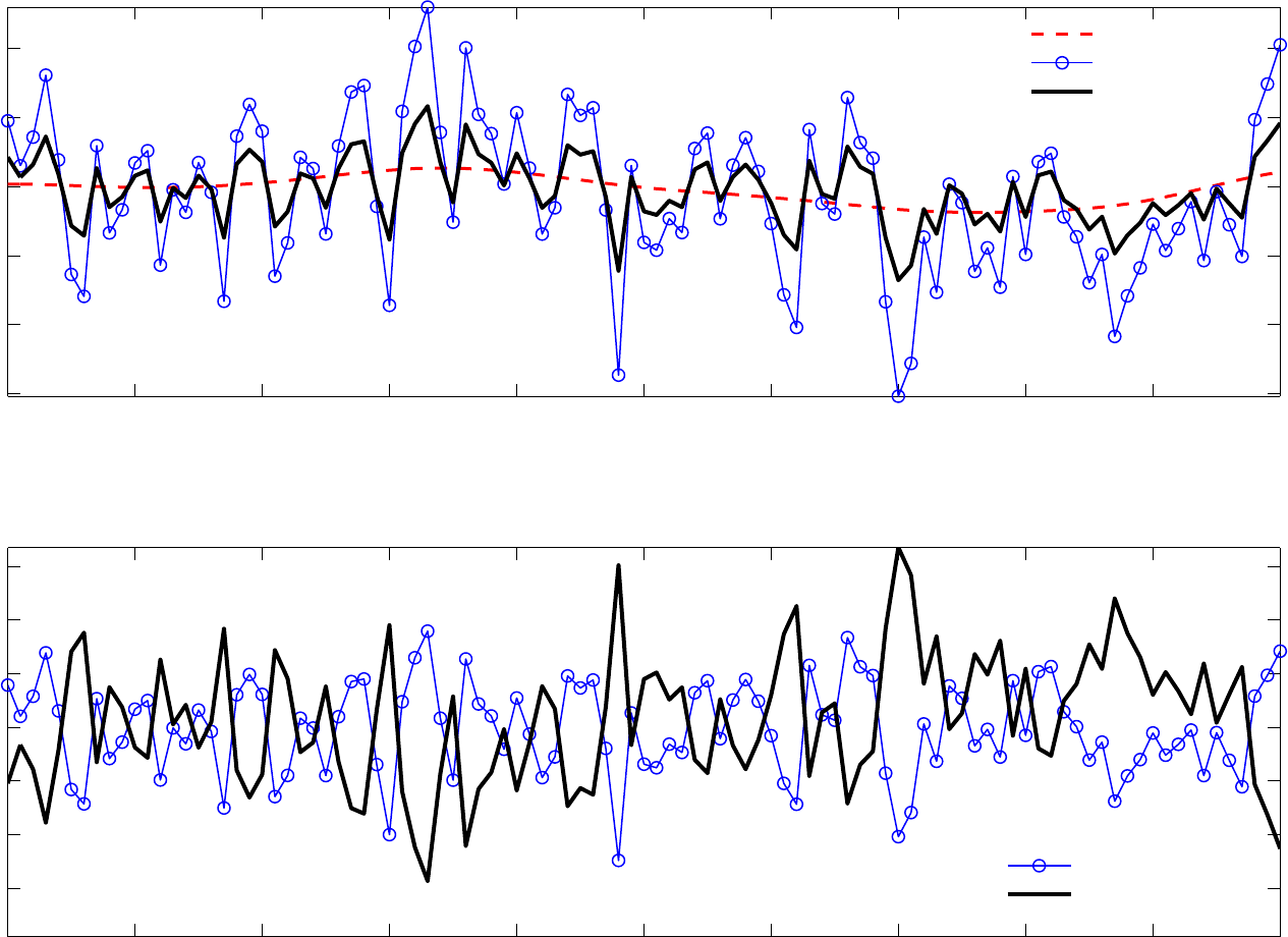
520 530 540 550 560 570 580 590 600 610 620

−3

−2

−1

Quarters

Percent

HP trend

Potential output

Actual output

Figure 9a: Potential Output, Actual Output and HP Trend Based on Actual Output (Simulated Data)

AR(1) in Levels Specification

520 530 540 550 560 570 580 590 600 610 620

−1.5

−1

−0.5

0.5

1.5

Quarters

Percent

Correlation(HP−filtered output and actual output gap) = −0.94

Std(actual gap) = 0.00629, Std(HP−filtered output) = 0.00457

HP−filtered output

Actual gap

Figure 9b: HP Filter Estimate of Output Gap Versus Actual Gap (Simulated Data)

AR(1) in Levels Specification

Figure 10: Dynamic Responses of Variables to a Monetary Policy Shock

0 5 10

−0.2

0.2

0.4

Real GDP (%)

0 5 10

−0.1

0.1

0.2

Inflation (GDP deflator, APR)

0 5 10

−0.6

−0.4

−0.2

0.2

Federal Funds Rate (APR)

0 5 10

−0.1

0.1

0.2

Real Consumption (%)

0 5 10

−0.5

0.5

Real Investment (%)

0 5 10

0.5

Capacity Utilization (%)

0 5 10

0.05

0.1

0.15

0.2

Rel. Price of Investment (%)

0 5 10

−0.1

0.1

0.2

0.3

Hours Worked Per Capita (%)

0 5 10

−0.15

−0.1

−0.05

0.05

Real Wage (%)

VAR 95% VAR Mean Medium−sized DSGE Model (Mean, 95%)

Figure 11: Dynamic Responses of Variables to a Neutral Technology Shock

0 5 10

0.2

0.4

0.6

Real GDP (%)

0 5 10

−0.8

−0.6

−0.4

−0.2

Inflation (GDP deflator, APR)

0 5 10

−0.4

−0.2

Federal Funds Rate (APR)

0 5 10

0.2

0.4

0.6

Real Consumption (%)

0 5 10

−0.5

0.5

1.5

Real Investment (%)

0 5 10

−0.5

0.5

Capacity Utilization (%)

0 5 10

−0.3

−0.2

−0.1

Rel. Price of Investment (%)

0 5 10

0.1

0.2

0.3

0.4

Hours Worked Per Capita (%)

0 5 10

0.1

0.2

0.3

0.4

Real Wage (%)

VAR 95% VAR Mean Medium−sized DSGE Model (Mean, 95%)

Figure 12: Dynamic Responses of Variables to an Investment Specific Technology Shock

0 5 10

0.2

0.4

0.6

Real GDP (%)

0 5 10

−0.4

−0.2

Inflation (GDP deflator, APR)

0 5 10

−0.2

0.2

0.4

Federal Funds Rate (APR)

0 5 10

0.2

0.4

0.6

Real Consumption (%)

0 5 10

−1

−0.5

0.5

Real Investment (%)

0 5 10

0.5

Capacity Utilization (%)

0 5 10

−0.6

−0.4

−0.2

Rel. Price of Investment (%)

0 5 10

0.2

0.4

Hours Worked Per Capita (%)

0 5 10

−0.2

−0.1

0.1

0.2

Real Wage (%)

VAR 95% VAR Mean Medium−sized DSGE Model (Mean, 95%)

Figure 13: VAR Specification Sensitivity: Response to a Monetary Policy Shock

5 10 15

−0.2

0.2

0.4

Real GDP (%)

Alternative VAR Specifications (All Combinations of:

VAR Lags 1,..,5 and Sample Starts 1951Q1,...,1985Q4)

VAR used for Estimation of the

Medium−sized DSGE Model (Mean, 95%)

5 10 15

−0.1

0.1

0.2

Inflation (GDP deflator, APR)

Alternative VAR Specifications (All Combinations of:

VAR Lags 1,..,5 and Sample Starts 1951Q1,...,1985Q4)

VAR used for Estimation of the

Medium−sized DSGE Model (Mean, 95%)

5 10 15

−0.6

−0.4

−0.2

0.2

Federal Funds Rate (APR)

Alternative VAR Specifications (All Combinations of:

VAR Lags 1,..,5 and Sample Starts 1951Q1,...,1985Q4)

VAR used for Estimation of the

Medium−sized DSGE Model (Mean, 95%)

5 10 15

−0.1

0.1

0.2

Real Consumption (%)

Alternative VAR Specifications (All Combinations of:

VAR Lags 1,..,5 and Sample Starts 1951Q1,...,1985Q4)

VAR used for Estimation of the

Medium−sized DSGE Model (Mean, 95%)

5 10 15

−0.5

0.5

Real Investment (%)

Alternative VAR Specifications (All Combinations of:

VAR Lags 1,..,5 and Sample Starts 1951Q1,...,1985Q4)

VAR used for Estimation of the

Medium−sized DSGE Model (Mean, 95%)

5 10 15

−0.2

0.2

0.4

0.6

0.8

Capacity Utilization (%)

Alternative VAR Specifications (All Combinations of:

VAR Lags 1,..,5 and Sample Starts 1951Q1,...,1985Q4)

VAR used for Estimation of the

Medium−sized DSGE Model (Mean, 95%)

5 10 15

−0.1

0.1

0.2

Rel. Price of Investment (%)

Alternative VAR Specifications (All Combinations of:

VAR Lags 1,..,5 and Sample Starts 1951Q1,...,1985Q4)

VAR used for Estimation of the

Medium−sized DSGE Model (Mean, 95%)

5 10 15

−0.1

0.1

0.2

0.3

Hours Worked Per Capita (%)

Alternative VAR Specifications (All Combinations of:

VAR Lags 1,..,5 and Sample Starts 1951Q1,...,1985Q4)

VAR used for Estimation of the

Medium−sized DSGE Model (Mean, 95%)

5 10 15

−0.1

0.1

Real Wage (%)

Alternative VAR Specifications (All Combinations of:

VAR Lags 1,..,5 and Sample Starts 1951Q1,...,1985Q4)

VAR used for Estimation of the

Medium−sized DSGE Model (Mean, 95%)

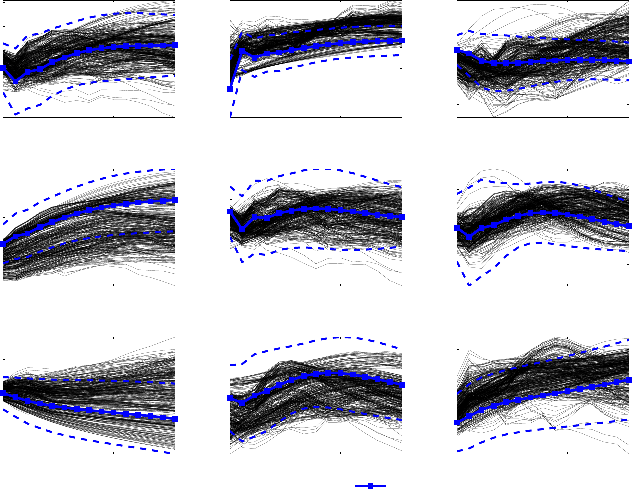
Figure 14: VAR Specification Sensitivity: Neutral Technology Shock

5 10 15

0.2

0.4

0.6

0.8

Real GDP (%)

Alternative VAR Specifications (All Combinations of:

VAR Lags 1,..,5 and Sample Starts 1951Q1,...,1985Q4)

VAR used for Estimation of the

Medium−sized DSGE Model (Mean, 95%)

5 10 15

−0.8

−0.6

−0.4

−0.2

0.2

Inflation (GDP deflator, APR)

Alternative VAR Specifications (All Combinations of:

VAR Lags 1,..,5 and Sample Starts 1951Q1,...,1985Q4)

VAR used for Estimation of the

Medium−sized DSGE Model (Mean, 95%)

5 10 15

−0.4

−0.2

0.2

Federal Funds Rate (APR)

Alternative VAR Specifications (All Combinations of:

VAR Lags 1,..,5 and Sample Starts 1951Q1,...,1985Q4)

VAR used for Estimation of the

Medium−sized DSGE Model (Mean, 95%)

5 10 15

0.2

0.4

0.6

Real Consumption (%)

Alternative VAR Specifications (All Combinations of:

VAR Lags 1,..,5 and Sample Starts 1951Q1,...,1985Q4)

VAR used for Estimation of the

Medium−sized DSGE Model (Mean, 95%)

5 10 15

−1

Real Investment (%)

Alternative VAR Specifications (All Combinations of:

VAR Lags 1,..,5 and Sample Starts 1951Q1,...,1985Q4)

VAR used for Estimation of the

Medium−sized DSGE Model (Mean, 95%)

5 10 15

−0.5

0.5

Capacity Utilization (%)

Alternative VAR Specifications (All Combinations of:

VAR Lags 1,..,5 and Sample Starts 1951Q1,...,1985Q4)

VAR used for Estimation of the

Medium−sized DSGE Model (Mean, 95%)

5 10 15

−0.2

0.2

Rel. Price of Investment (%)

Alternative VAR Specifications (All Combinations of:

VAR Lags 1,..,5 and Sample Starts 1951Q1,...,1985Q4)

VAR used for Estimation of the

Medium−sized DSGE Model (Mean, 95%)

5 10 15

0.2

0.4

Hours Worked Per Capita (%)

Alternative VAR Specifications (All Combinations of:

VAR Lags 1,..,5 and Sample Starts 1951Q1,...,1985Q4)

VAR used for Estimation of the

Medium−sized DSGE Model (Mean, 95%)

5 10 15

0.2

0.4

Real Wage (%)

Alternative VAR Specifications (All Combinations of:

VAR Lags 1,..,5 and Sample Starts 1951Q1,...,1985Q4)

VAR used for Estimation of the

Medium−sized DSGE Model (Mean, 95%)

Figure 15: VAR Specification Sensitivity: Investment Specific Technology Shock

5 10 15

−0.4

−0.2

0.2

0.4

0.6

Real GDP (%)

Alternative VAR Specifications (All Combinations of:

VAR Lags 1,..,5 and Sample Starts 1951Q1,...,1985Q4)

VAR used for Estimation of the

Medium−sized DSGE Model (Mean, 95%)

5 10 15

−0.4

−0.2

0.2

0.4

Inflation (GDP deflator, APR)

Alternative VAR Specifications (All Combinations of:

VAR Lags 1,..,5 and Sample Starts 1951Q1,...,1985Q4)

VAR used for Estimation of the

Medium−sized DSGE Model (Mean, 95%)

5 10 15

−0.5

0.5

Federal Funds Rate (APR)

Alternative VAR Specifications (All Combinations of:

VAR Lags 1,..,5 and Sample Starts 1951Q1,...,1985Q4)

VAR used for Estimation of the

Medium−sized DSGE Model (Mean, 95%)

5 10 15

−0.2

0.2

0.4

0.6

Real Consumption (%)

Alternative VAR Specifications (All Combinations of:

VAR Lags 1,..,5 and Sample Starts 1951Q1,...,1985Q4)

VAR used for Estimation of the

Medium−sized DSGE Model (Mean, 95%)

5 10 15

−1

Real Investment (%)

Alternative VAR Specifications (All Combinations of:

VAR Lags 1,..,5 and Sample Starts 1951Q1,...,1985Q4)

VAR used for Estimation of the

Medium−sized DSGE Model (Mean, 95%)

5 10 15

−0.5

0.5

Capacity Utilization (%)

Alternative VAR Specifications (All Combinations of:

VAR Lags 1,..,5 and Sample Starts 1951Q1,...,1985Q4)

VAR used for Estimation of the

Medium−sized DSGE Model (Mean, 95%)

5 10 15

−0.6

−0.4

−0.2

Rel. Price of Investment (%)

Alternative VAR Specifications (All Combinations of:

VAR Lags 1,..,5 and Sample Starts 1951Q1,...,1985Q4)

VAR used for Estimation of the

Medium−sized DSGE Model (Mean, 95%)

5 10 15

−0.2

0.2

0.4

Hours Worked Per Capita (%)

Alternative VAR Specifications (All Combinations of:

VAR Lags 1,..,5 and Sample Starts 1951Q1,...,1985Q4)

VAR used for Estimation of the

Medium−sized DSGE Model (Mean, 95%)

5 10 15

−0.2

0.2

0.4

Real Wage (%)

Alternative VAR Specifications (All Combinations of:

VAR Lags 1,..,5 and Sample Starts 1951Q1,...,1985Q4)

VAR used for Estimation of the

Medium−sized DSGE Model (Mean, 95%)

0.2 0.4 0.6

0.2 0.4 0.6 0.8 1

0.1 0.2 0.3 0.4 0.5

0.2 0.4 0.6 0.8

0.1 0.2 0.3 0.4 0.5

0.5 0.6 0.7 0.8 0.9

1.2 1.4 1.6 1.8 2

0 0.2 0.4 0.6

10 20 30

0.05

0.1

0.15

”

0.4 0.6 0.8

1 2 3

1.2 1.4 1.6

Prior

Posterior (Laplace Approximation After Posterior Mode Optimization)

Posterior Mode (After Posterior Mode Optimization)

Posterior (After Random Walk Metropolis (MCMC), Kernel Estimate)

Figure 16: Priors and Posteriors of Estimated Parameters of the Medium−Sized DSGE Model

0.2 0.4 0.6 0.8