
Springer Texts in Statistics
PeterK.Dunn· GordonK.Smyth
Generalized
Linear Models
With Examples
in R

Springer Texts in Statistics
Series Editors
R. DeVeaux
S.E. Fienberg
I. Olkin
Peter K. Dunn • Gordon K. Smyth
Generalized Linear Models
With Examples in R
123
Peter K. Dunn
Faculty of Science, Health, Education
and Engineering
School of Health of Sport Science
University of the Sunshine Coast
QLD, Australia
Gordon K. Smyth
Bioinformatics Division
Walter and Eliza Hall Institute
of Medical Research
Parkville, VIC, Australia
ISSN 1431-875X ISSN 2197-4136 (electronic)
Springer Texts in Statistics
ISBN 978-1-4419-0117-0 ISBN 978-1-4419-0118-7 (eBook)
https://doi.org/10.1007/978-1-4419-0118-7
Library of Congress Control Number: 2018954737
© Springer Science+Business Media, LLC, part of Springer Nature 2018
This work is subject to copyright. All rights are reserved by the Publisher, whether the whole or part of
the material is concerned, specifically the rights of translation, reprinting, reuse of illustrations, recitation,
broadcasting, reproduction on microfilms or in any other physical way, and transmission or information
storage and retrieval, electronic adaptation, computer software, or by similar or dissimilar methodology
now known or hereafter developed.
The use of general descriptive names, registered names, trademarks, service marks, etc. in this publication
does not imply, even in the absence of a specific statement, that such names are exempt from the relevant
protective laws and regulations and therefore free for general use.
The publisher, the authors, and the editors are safe to assume that the advice and information in this book
are believed to be true and accurate at the date of publication. Neither the publisher nor the authors or
the editors give a warranty, express or implied, with respect to the material contained herein or for any
errors or omissions that may have been made. The publisher remains neutral with regard to jurisdictional
claims in published maps and institutional affiliations.
This Springer imprint is published by the registered company Springer Science+Business Media, LLC
part of Springer Nature.
The registered company address is: 233 Spring Street, New York, NY 10013, U.S.A.
To my wife Alison; our children Jessica,
Emily, Jemima, Samuel, Josiah and
Elijah; and my parents: Thank you for
your love and support and for giving so
much so I could get this far. PKD
To those who taught me about glms 40
years ago and to all the students who, in
the years since, have patiently listened to
me on the subject, given feedback and
generally made it rewarding to be a
teacher. GKS
Preface
A sophisticated analysis is wasted if the results cannot be
communicated effectively to the client.
Reese [4, p. 201]
Our purpose in writing this book is to combine a good applied introduction to
generalized linear models (glms) with a thorough explanation of the theory
that is understandable from an elementary point of view.
We assume students to have basic knowledge of statistics and calculus. A
working familiarity with probability, probability distributions and hypothe-
sis testing is assumed, but a self-contained introduction to all other topics is
given in the book including linear regression. The early chapters of the book
give an introduction to linear regression and analysis of variance suitable
for a second course in statistics. Students with more advanced backgrounds,
including matrix algebra, will benefit from optional sections that give a de-
tailed introduction to the theory and algorithms. The book can therefore be
read at multiple levels. It can be read by students with only a first course in
statistics, but at the same time, it contains advanced material suitable for
graduate students and professionals.
The book should be appropriate for graduate students in statistics at either
the masters or PhD levels. It should be also be appropriate for advanced
undergraduate students taking majors in statistics in Britain or Australia.
Students in psychology, biometrics and related disciplines will also benefit.
In general, it is appropriate for anyone wanting a practical working knowledge
of glms with a sound theoretical background.
r is a powerful and freely available environment for statistical computing
and graphics that has become widely adopted around the world. This book
includes a self-contained introduction to R (Appendix A), and use of r is
integrated into the text throughout the book. This includes comprehensive
r code examples and complete code for most data analyses and case studies.
Detailed use of relevant r functions is described in each chapter.
A practical working knowledge of good applied statistical practice is de-
veloped through the use of real data sets and numerous case studies. This
book makes almost exclusive use of real data. These data sets are collected in
the r package GLMsData [1] (see Appendix A for instructions for obtaining
vii
viii Preface
this r package), which has been prepared especially for use with this book
and which contains 97 data sets. Each example in the text is cross-referenced
with the relevant data set so that readers can load the relevant data to follow
the analysis in their own r session. Complete reproducible r code is provided
with the text for most examples.
The development of the theoretical background sometimes requires more
advanced mathematical techniques, including the use of matrix algebra. How-
ever, knowledge of these techniques is not required to read this book. We have
ensured that readers without this knowledge can still follow the theoretical
development, by flagging the corresponding sections with a star * in the*
margin. Readers unfamiliar with these techniques may skip these sections
and problems without loss of continuity. However, those with the necessary
knowledge can gain more insight by reading the optional starred sections.
A set of problems is given at the end of each chapter and at the end of the
book. The balance between theory and practice is evident in the list of prob-
lems, which vary in difficulty and purpose. These problems cover many areas
of application and test understanding, theory, application, interpretation and
the ability to read publications that use glms.
This book begins with an introduction to multiple linear regression. In
abookaboutglms, at least three reasons exist for beginning with a short
discussion of multiple linear regression:
• Linear regression is familiar. Starting with regression consolidates this
material and establishes common notation, terminology and knowledge
for all readers. Notation and new terms are best introduced in a familiar
context.
• Linear regression is foundational. Many concepts and ideas from linear
regression are used as approximations in glms. A firm foundation in
linear regression ensures a better understanding of glms.
• Linear regression is motivational. Glmsoftenimprove linear regression.
Studying linear regression reveals its weaknesses and shows how glms
can often overcome most of these, motivating the need for glms.
Connections between linear regression and glms are emphasized throughout
this book.
This book contains a number of important but advanced topics and tools
that have not typically been included in introductions to glms before. These
include Tweedie family distributions with power variance functions, saddle-
point approximations, likelihood score tests, modified profile likelihood and
randomized quantile residuals, as well as regression splines and orthogonal
polynomials. Particular features are the use of saddlepoint approximations
to clarify the asymptotical distribution of residual deviances from glmsand
an explanation of the relationship between score tests and Pearson statis-
tics. Practical and specific guidelines are developed for the use of asymptotic
approximations.
Preface ix
Throughout this book, r functions are shown in typewriter font fol-
lowed by parentheses; for example, glm(). Operators, data frames and vari-
ables in r are shown in typewriter font; for example, Smoke. r packages
are shown in bold and sans serif font; for example, GLMsData.
We thank those who have contributed to the writing of this book and
especially students who have contributed to earlier versions of this text. We
particularly thank Janette Benson, Alison Howes and Martine Maron for the
permission to use data.
This book was prepared using L
A
T
E
Xandr version 3.4.3 [3], integrated
using Sweave [2].
Sippy Downs, QLD, Australia Peter K. Dunn
Parkville, VIC, Australia Gordon K. Smyth
December 2017
References
[1] Dunn, P.K., Smyth, G.K.: GLMsData: Generalized linear model data sets
(2017). URL https://CRAN.R-project.org/package=GLMsData. R pack-
age version 1.0.0
[2] Leisch, F.: Dynamic generation of statistical reports using literate data
analysis. In: W. Härdle, B. Rönz (eds.) Compstat 2002—Proceedings
in Computational Statistics, pp. 575–580. Physika Verlag, Heidelberg,
Germany (2002)
[3] R Development Core Team: R: A Language and Environment for Statisti-
cal Computing. R Foundation for Statistical Computing, Vienna, Austria
(2017). URL https://www.R-project.org
[4] Reese, R.A.: Data analysis: The need for models? The Statistician 35(2),
199–206 (1986). Special Issue: Statistical Modelling
Contents
1 Statistical Models ......................................... 1
1.1 Introduction and Overview .............................. 1
1.2 Conventions for Describing Data ......................... 1
1.3 Plotting Data ......................................... 5
1.4 Coding for Factors ..................................... 10
1.5 Statistical Models Describe Both Random and Systematic
Features of Data ....................................... 11
1.6 Regression Models ..................................... 12
1.7 Interpreting Regression Models .......................... 16
1.8 All Models Are Wrong, but Some Are Useful .............. 17
1.9 The Purpose of a Statistical Model Affects How It Is
Developed ............................................ 18
1.10 Accuracy vs Parsimony ................................. 19
1.11 Experiments vs Observational Studies: Causality
vs Association ......................................... 21
1.12 Data Collection and Generalizability ..................... 22
1.13 Using R for Statistical Modelling ........................ 23
1.14 Summary ............................................. 24
Problems ................................................... 25
References .................................................. 29
2 Linear Regression Models ................................. 31
2.1 Introduction and Overview .............................. 31
2.2 Linear Regression Models Defined ........................ 31
2.3 Simple Linear Regression ............................... 35
2.3.1 Least-Squares Estimation ........................ 35
2.3.2 Coefficient Estimates ............................ 36
2.3.3 Estimating the Variance σ
2
...................... 38
2.3.4 Standard Errors of the Coefficients ................ 39
2.3.5 Standard Errors of Fitted Values ................. 39
xi
xii Contents
2.4 Estimation for Multiple Regression ....................... 40
2.4.1 Coefficient Estimates ............................ 40
2.4.2 Estimating the Variance σ
2
...................... 42
2.4.3 Standard Errors ................................ 42
* 2.5 Matrix Formulation of Linear Regression Models ........... 43
* 2.5.1 Matrix Notation ................................ 43
* 2.5.2 Coefficient Estimates ............................ 44
* 2.5.3 Estimating the Variance σ
2
...................... 46
* 2.5.4 Estimating the Variance of
ˆ
β ..................... 47
* 2.5.5 Estimating the Variance of Fitted Values .......... 47
2.6 Fitting Linear Regression Models Using R ................ 48
2.7 Interpreting the Regression Coefficients ................... 52
2.8 Inference for Linear Regression Models: t-Tests ............ 53
2.8.1 Normal Linear Regression Models ................. 53
2.8.2 The Distribution of
ˆ
β
j
........................... 53
2.8.3 Hypothesis Tests for β
j
.......................... 54
2.8.4 Confidence Intervals for β
j
....................... 55
2.8.5 Confidence Intervals for μ ........................ 56
2.9 Analysis of Variance for Regression Models ................ 58
2.10 Comparing Nested Models .............................. 61
2.10.1 Analysis of Variance to Compare Two Nested
Models ........................................ 61
2.10.2 Sequential Analysis of Variance ................... 63
2.10.3 Parallel and Independent Regressions .............. 66
2.10.4 The Marginality Principle ........................ 70
2.11 Choosing Between Non-nested Models: AIC and BIC ....... 70
2.12 Tools to Assist in Model Selection........................ 72
2.12.1 Adding and Dropping Variables................... 72
2.12.2 Automated Methods for Model Selection ........... 73
2.12.3 Objections to Using Stepwise Procedures .......... 76
2.13 Case Study ........................................... 76
2.14 Using R for Fitting Linear Regression Models ............. 79
2.15 Summary ............................................. 82
Problems ................................................... 83
References .................................................. 90
3 Linear Regression Models: Diagnostics
and Model-Building ....................................... 93
3.1 Introduction and Overview .............................. 93
3.2 Assumptions from a Practical Point of View ............... 94
3.2.1 Types of Assumptions ........................... 94
3.2.2 The Linear Predictor ............................ 94
3.2.3 Constant Variance .............................. 94
3.2.4 Independence .................................. 95
3.2.5 Normality ..................................... 96
Contents xiii
3.2.6 Measurement Scales ............................. 96
3.2.7 Approximations and Consequences ................ 96
3.3 Residuals for Normal Linear Regression Models ............ 97
3.4 The Leverages for Linear Regression Models ............... 98
3.4.1 Leverage and Extreme Covariate Values ........... 98
* 3.4.2 The Leverages Using Matrix Algebra .............. 100
3.5 Residual Plots ......................................... 101
3.5.1 Plot Residuals Against x
j
: Linearity .............. 101
3.5.2 Partial Residual Plots ........................... 102
3.5.3 Plot Residuals Against ˆμ: Constant Variance ....... 104
3.5.4 Q–Q Plots and Normality ........................ 105
3.5.5 Lag Plots and Dependence over Time ............. 106
3.6 Outliers and Influential Observations ..................... 108
3.6.1 Introduction ................................... 108
3.6.2 Outliers and Studentized Residuals ............... 109
3.6.3 Influential Observations ......................... 110
3.7 Terminology for Residuals .............................. 115
3.8 Remedies: Fixing Identified Problems ..................... 115
3.9 Transforming the Response ............................. 116
3.9.1 Symmetry, Constraints and the Ladder of Powers ... 116
3.9.2 Variance-Stabilizing Transformations .............. 117
3.9.3 Box–Cox Transformations........................ 120
3.10 Simple Transformations of Covariates ..................... 121
3.11 Polynomial Trends ..................................... 127
3.12 Regression Splines ..................................... 131
3.13 Fixing Identified Outliers ............................... 134
3.14 Collinearity ........................................... 135
3.15 Case Studies .......................................... 138
3.15.1 Case Study 1 ................................... 138
3.15.2 Case Study 2 ................................... 141
3.16 Using R for Diagnostic Analysis of Linear Regression
Models ............................................... 146
3.17 Summary ............................................. 147
Problems ................................................... 149
References .................................................. 162
4 Beyond Linear Regression: The Method of Maximum
Likelihood ................................................ 165
4.1 Introduction and Overview .............................. 165
4.2 The Need for Non-normal Regression Models .............. 165
4.2.1 When Linear Models Are a Poor Choice ........... 165
4.2.2 Binary Outcomes and Binomial Counts ............ 166
4.2.3 Unrestricted Counts: Poisson or Negative Binomial . . 168
4.2.4 Continuous Positive Observations ................. 169
4.3 Generalizing the Normal Linear Model ................... 171
xiv Contents
4.4 The Idea of Likelihood Estimation ....................... 172
4.5 Maximum Likelihood for Estimating One Parameter ....... 176
4.5.1 Score Equations ................................ 176
4.5.2 Information: Observed and Expected .............. 177
4.5.3 Standard Errors of Parameters ................... 179
4.6 Maximum Likelihood for More Than One Parameter ....... 180
4.6.1 Score Equations ................................ 180
4.6.2 Information: Observed and Expected .............. 182
4.6.3 Standard Errors of Parameters ................... 183
* 4.7 Maximum Likelihood Using Matrix Algebra ............... 183
* 4.7.1 Notation ....................................... 183
* 4.7.2 Score Equations ................................ 183
* 4.7.3 Information: Observed and Expected .............. 184
* 4.7.4 Standard Errors of Parameters ................... 186
* 4.8 Fisher Scoring for Computing MLEs ..................... 186
4.9 Properties of MLEs .................................... 189
4.9.1 Introduction ................................... 189
4.9.2 Properties of MLEs for One Parameter ............ 189
* 4.9.3 Properties of MLEs for Many Parameters .......... 190
4.10 Hypothesis Testing: Large Sample Asymptotic Results ...... 191
4.10.1 Introduction ................................... 191
* 4.10.2 Global Tests ................................... 194
* 4.10.3 Tests About Subsets of Parameters ............... 196
4.10.4 Tests About One Parameter in a Set of Parameters . 197
4.10.5 Comparing the Three Methods ................... 199
4.11 Confidence Intervals .................................... 200
* 4.11.1 Confidence Regions for More Than One Parameter . . 200
4.11.2 Confidence Intervals for Single Parameters ......... 200
4.12 Comparing Non-nested Models: The AIC and BIC ......... 202
4.13 Summary ............................................. 204
* 4.14 Appendix: R Code to Fit Models to the Quilpie Rainfall
Data ................................................. 204
Problems ................................................... 206
References .................................................. 209
5 Generalized Linear Models: Structure ..................... 211
5.1 Introduction and Overview .............................. 211
5.2 The Two Components of Generalized Linear Models ........ 211
5.3 The Random Component: Exponential Dispersion Models . . . 212
5.3.1 Examples of EDMs ............................. 212
5.3.2 Definition of EDMs ............................. 212
5.3.3 Generating Functions ........................... 214
5.3.4 The Moment Generating and Cumulant Functions
for EDMs ...................................... 215
5.3.5 The Mean and Variance of an EDM ............... 216
Contents xv
5.3.6 The Variance Function .......................... 217
5.4 EDMs in Dispersion Model Form ........................ 218
5.4.1 The Unit Deviance and the Dispersion Model Form ... 218
5.4.2 The Saddlepoint Approximation .................. 223
5.4.3 The Distribution of the Unit Deviance ............. 224
5.4.4 Accuracy of the Saddlepoint Approximation ........ 225
5.4.5 Accuracy of the χ
2
1
Distribution for the Unit
Deviance ...................................... 226
5.5 The Systematic Component ............................. 229
5.5.1 Link Function .................................. 229
5.5.2 Offsets ........................................ 229
5.6 Generalized Linear Models Defined ....................... 230
5.7 The Total Deviance .................................... 231
5.8 Regression Transformations Approximate GLMs ........... 232
5.9 Summary ............................................. 234
Problems ................................................... 235
References .................................................. 240
6 Generalized Linear Models: Estimation ................... 243
6.1 Introduction and Overview .............................. 243
6.2 Likelihood Calculations for β ............................ 243
6.2.1 Differentiating the Probability Function ........... 243
6.2.2 Score Equations and Information for β ............ 244
6.3 Computing Estimates of β .............................. 245
6.4 The Residual Deviance ................................. 248
6.5 Standard Errors for
ˆ
β .................................. 250
* 6.6 Estimation of β: Matrix Formulation ..................... 250
6.7 Estimation of GLMs Is Locally Like Linear Regression ...... 252
6.8 Estimating φ .......................................... 252
6.8.1 Introduction ................................... 252
6.8.2 The Maximum Likelihood Estimator of φ .......... 253
6.8.3 Modified Profile Log-Likelihood Estimator of φ ..... 253
6.8.4 Mean Deviance Estimator of φ ................... 254
6.8.5 Pearson Estimator of φ .......................... 255
6.8.6 Which Estimator of φ Is Best? ................... 255
6.9 Using R to Fit GLMs .................................. 257
6.10 Summary ............................................. 259
Problems ................................................... 261
References .................................................. 262
7 Generalized Linear Models: Inference ..................... 265
7.1 Introduction and Overview .............................. 265
7.2 Inference for Coefficients When φ Is Known ............... 265
7.2.1 Wald Tests for Single Regression Coefficients ....... 265
7.2.2 Confidence Intervals for Individual Coefficients ..... 266
xvi Contents
7.2.3 Confidence Intervals for μ ........................ 267
7.2.4 Likelihood Ratio Tests to Compare Nested Models:
χ
2
Tests ....................................... 269
7.2.5 Analysis of Deviance Tables to Compare Nested
Models ........................................ 270
7.2.6 Score Tests .................................... 271
* 7.2.7 Score Tests Using Matrices ....................... 272
7.3 Large Sample Asymptotics .............................. 273
7.4 Goodness-of-Fit Tests with φ Known ..................... 274
7.4.1 The Idea of Goodness-of-Fit ...................... 274
7.4.2 Deviance Goodness-of-Fit Test ................... 275
7.4.3 Pearson Goodness-of-Fit Test .................... 275
7.5 Small Dispersion Asymptotics ........................... 276
7.6 Inference for Coefficients When φ Is Unknown ............. 278
7.6.1 Wald Tests for Single Regression Coefficients ....... 278
7.6.2 Confidence Intervals for Individual Coefficients ..... 280
* 7.6.3 Confidence Intervals for μ ........................ 281
7.6.4 Likelihood Ratio Tests to Compare Nested Models:
F -Tests ........................................ 282
7.6.5 Analysis of Deviance Tables to Compare Nested
Models ........................................ 284
7.6.6 Score Tests .................................... 286
7.7 Comparing Wald, Score and Likelihood Ratio Tests ........ 287
7.8 Choosing Between Non-nested GLMs: AIC and BIC ........ 288
7.9 Automated Methods for Model Selection .................. 289
7.10 Using R to Perform Tests ............................... 290
7.11 Summary ............................................. 292
Problems ................................................... 293
References .................................................. 296
8 Generalized Linear Models: Diagnostics ................... 297
8.1 Introduction and Overview .............................. 297
8.2 Assumptions of GLMs .................................. 297
8.3 Residuals for GLMs .................................... 298
8.3.1 Response Residuals Are Insufficient for GLMs ...... 298
8.3.2 Pearson Residuals .............................. 299
8.3.3 Deviance Residuals ............................. 300
8.3.4 Quantile Residuals .............................. 300
8.4 The Leverages in GLMs ................................ 304
8.4.1 Working Leverages .............................. 304
* 8.4.2 The Hat Matrix ................................ 304
8.5 Leverage Standardized Residuals for GLMs ............... 305
8.6 When to Use Which Type of Residual .................... 306
8.7 Checking the Model Assumptions ........................ 306
8.7.1 Introduction ................................... 306
Contents xvii
8.7.2 Independence: Plot Residuals Against Lagged
Residuals ...................................... 307
8.7.3 Plots to Check the Systematic Component ......... 307
8.7.4 Plots to Check the Random Component ........... 311
8.8 Outliers and Influential Observations ..................... 312
8.8.1 Introduction ................................... 312
8.8.2 Outliers and Studentized Residuals ............... 312
8.8.3 Influential Observations ......................... 313
8.9 Remedies: Fixing Identified Problems ..................... 315
8.10 Quasi-Likelihood and Extended Quasi-Likelihood .......... 318
8.11 Collinearity ........................................... 321
8.12 Case Study ........................................... 322
8.13 Using R for Diagnostic Analysis of GLMs ................. 325
8.14 Summary ............................................. 326
Problems ................................................... 327
References .................................................. 330
9 Models for Proportions: Binomial GLMs .................. 333
9.1 Introduction and Overview .............................. 333
9.2 Modelling Proportions .................................. 333
9.3 Link Functions ........................................ 336
9.4 Tolerance Distributions and the Probit Link ............... 338
9.5 Odds, Odds Ratios and the Logit Link .................... 340
9.6 Median Effective Dose, ED50 ............................ 343
9.7 The Complementary Log-Log Link in Assay Analysis ....... 344
9.8 Overdispersion ........................................ 347
9.9 When Wald Tests Fail .................................. 351
9.10 No Goodness-of-Fit for Binary Responses ................. 354
9.11 Case Study ........................................... 354
9.12 Using R to Fit GLMs to Proportion Data ................. 360
9.13 Summary ............................................. 360
Problems ................................................... 361
References .................................................. 367
10 Models for Counts: Poisson and Negative Binomial GLMs 371
10.1 Introduction and Overview .............................. 371
10.2 Summary of Poisson GLMs ............................. 371
10.3 Modelling Rates ....................................... 373
10.4 Contingency Tables: Log-Linear Models ................... 378
10.4.1 Introduction ................................... 378
10.4.2 Two Dimensional Tables: Systematic Component ... 378
10.4.3 Two-Dimensional Tables: Random Components ..... 380
10.4.4 Three-Dimensional Tables ....................... 385
10.4.5 Simpson’s Paradox .............................. 389
10.4.6 Equivalence of Binomial and Poisson GLMs ........ 392
xviii Contents
10.4.7 Higher-Order Tables ............................ 393
10.4.8 Structural Zeros in Contingency Tables ............ 395
10.5 Overdispersion ........................................ 397
10.5.1 Overdispersion for Poisson GLMs ................. 397
10.5.2 Negative Binomial GLMs ........................ 399
10.5.3 Quasi-Poisson Models ........................... 402
10.6 Case Study ........................................... 404
10.7 Using R to Fit GLMs to Count Data ..................... 411
10.8 Summary ............................................. 411
Problems ................................................... 412
References .................................................. 422
11 Positive Continuous Data: Gamma and Inverse Gaussian
GLMs ..................................................... 425
11.1 Introduction and Overview .............................. 425
11.2 Modelling Positive Continuous Data ...................... 425
11.3 The Gamma Distribution ............................... 427
11.4 The Inverse Gaussian Distribution ....................... 431
11.5 Link Functions ........................................ 433
11.6 Estimating the Dispersion Parameter ..................... 436
11.6.1 Estimating φ for the Gamma Distribution ......... 436
11.6.2 Estimating φ for the Inverse Gaussian Distribution . . 439
11.7 Case Studies .......................................... 440
11.7.1 Case Study 1 ................................... 440
11.7.2 Case Study 2 ................................... 442
11.8 Using R to Fit Gamma and Inverse Gaussian GLMS ....... 445
11.9 Summary ............................................. 445
Problems ................................................... 446
References .................................................. 454
12 Tweedie GLMs ............................................ 457
12.1 Introduction and Overview .............................. 457
12.2 The Tweedie EDMs .................................... 457
12.2.1 Introducing Tweedie Distributions ................ 457
12.2.2 The Structure of Tweedie EDMs .................. 460
12.2.3 Tweedie EDMs for Positive Continuous Data ....... 461
12.2.4 Tweedie EDMs for Positive Continuous Data with
Exact Zeros .................................... 463
12.3 Tweedie GLMs ........................................ 464
12.3.1 Introduction ................................... 464
12.3.2 Estimation of the Index Parameter ξ .............. 465
12.3.3 Fitting Tweedie GLMs .......................... 469
12.4 Case Studies .......................................... 473
12.4.1 Case Study 1 ................................... 473
12.4.2 Case Study 2 ................................... 475
Contents xix
12.5 Using R to Fit Tweedie GLMs ........................... 478
12.6 Summary ............................................. 479
Problems ................................................... 480
References .................................................. 488
13 Extra Problems ........................................... 491
13.1 Introduction and Overview .............................. 491
Problems ................................................... 491
References .................................................. 500
Using R for Data Analysis .................................... 503
A.1 Introduction and Overview .............................. 503
A.2 Preparing to Use R .................................... 503
A.2.1 Introduction to R ............................... 503
A.2.2 Important R Websites ........................... 504
A.2.3 Obtaining and Installing R ....................... 504
A.2.4 Downloading and Installing R Packages ............ 504
A.2.5 Using R Packages ............................... 505
A.2.6 The R Packages Used in This Book ............... 506
A.3 Introduction to Using R ................................ 506
A.3.1 Basic Use of R as an Advanced Calculator ......... 506
A.3.2 Quitting R ..................................... 508
A.3.3 Obtaining Help in R ............................ 508
A.3.4 Variable Names in R ............................ 508
A.3.5 Working with Vectors in R ....................... 509
A.3.6 Loading Data into R ............................ 511
A.3.7 Working with Data Frames in R .................. 513
A.3.8 Using Functions in R ............................ 514
A.3.9 Basic Statistical Functions in R ................... 515
A.3.10 Basic Plotting in R ............................. 516
A.3.11 Writing Functions in R .......................... 518
* A.3.12 Matrix Arithmetic in R .......................... 520
References .................................................. 523
The GLMsData package ....................................... 525
References .................................................. 527
Selected Solutions ............................................ 529
Solutions from Chap. 1 ....................................... 529
Solutions from Chap. 2 ....................................... 530
Solutions from Chap. 3 ....................................... 532
Solutions from Chap. 4 ....................................... 534
Solutions from Chap. 5 ....................................... 536
Solutions from Chap. 6 ....................................... 537
Solutions from Chap. 7 ....................................... 537
Solutions from Chap. 8 ....................................... 539
xx Contents
Solutions from Chap. 9 ....................................... 539
Solutions from Chap. 10 ...................................... 541
Solutions from Chap. 11 ...................................... 544
Solutions from Chap. 12 ...................................... 547
Solutions from Chap. 13 ...................................... 548
References .................................................. 550
Index: Data sets .............................................. 551
Index: R commands .......................................... 553
Index: General topics ......................................... 557

Chapter 1
Statistical Models
...all models are approximations. Essentially, all models
are wrong, but some are useful. However, the approximate
nature of the model must always be borne in mind.
Box and Draper [2, p. 424]
1.1 Introduction and Overview
This chapter introduces the concept of a statistical model. One particular
type of statistical model—the generalized linear model—is the focus of this
book, and so we begin with an introduction to statistical models in gen-
eral. This allows us to introduce the necessary language, notation, and other
important issues. We first discuss conventions for describing data mathemati-
cally (Sect. 1.2). We then highlight the importance of plotting data (Sect. 1.3),
and explain how to numerically code non-numerical variables (Sect. 1.4)so
that they can be used in mathematical models. We then introduce the two
components of a statistical model used for understanding data (Sect. 1.5):
the systematic and random components. The class of regression models is
then introduced (Sect. 1.6), which includes all models in this book. Model
interpretation is then considered (Sect. 1.7), followed by comparing physical
models and statistical models (Sect. 1.8) to highlight the similarities and dif-
ferences. The purpose of a statistical model is then given (Sect. 1.9), followed
by a description of the two criteria for evaluating statistical models: accuracy
and parsimony (Sect. 1.10). The importance of understanding the limitations
of statistical models is then addressed (Sect. 1.11), including the differences
between observational and experimental data. The generalizability of models
is then discussed (Sect. 1.12). Finally, we make some introductory comments
about using r for statistical modelling (Sect. 1.13).
1.2 Conventions for Describing Data
The concepts in this chapter are best introduced using an example.
Example 1.1. A study of 654 youths in East Boston [10, 18, 20] explored the
relationships between lung capacity (measured by forced expiratory volume,
© Springer Science+Business Media, LLC, part of Springer Nature 2018
P. K. Dunn, G. K. Smyth, Generalized Linear Models with Examples in R,
Springer Texts in Statistics, https://doi.org/10.1007/978-1-4419-0118-7_1
1

21StatisticalModels
or fev, in litres) and smoking status, age, height and gender (Table 1.1). The
data are available in r as the data frame lungcap (short for ‘lung capacity’),
part of the GLMsData package [4]. For information about this package, see
Appendix B; for more information about r, see Appendix A. Assuming the
GLMsData package is installed in r (see Sect. A.2.4), load the GLMsData
package and the lungcap data frame as follows:
> library(GLMsData) # Load the GLMsData package
> data(lungcap) # Make the data set lungcap available for use
> head(lungcap) # Show the first few lines of data
Age FEV Ht Gender Smoke
1 3 1.072 46 F 0
2 4 0.839 48 F 0
3 4 1.102 48 F 0
4 4 1.389 48 F 0
5 4 1.577 49 F 0
6 4 1.418 49 F 0
(The # character and all subsequent text is ignored by r.) The data frame
lungcap consist of five variables: Age, FEV, Ht, Gender and Smoke. Some
of these variables are numerical variables (such as Age), and some are non-
numerical variables (such as Gender). Any one of these can be accessed indi-
vidually using $ as follows:
> head(lungcap$Age) # Show first six values of Age
[1]344444
> tail(lungcap$Gender) # Show last six values of Gender
[1]MMMMMM
Levels: F M
Tabl e 1. 1 The forced expiratory volume (fev) of youths, sampled from East Boston
during the middle to late 1970s. fev is in L; age is in completed years; height is in inches.
The complete data set consists of 654 observations in total (Example 1.1)
Non-smokers Smokers
Females Males Females Males
fev Age Height fev Age Height fev Age Height fev Age Height
1.072 3 46.0 1.404 3 51.5 2.975 10 63.0 1.953 9 58.0
0.839 4 48.0 0.796 4 47.0 3.038 10 65.0 3.498 10 68.0
1.102 4 48.0 1.004 4 48.0 2.387 10 66.0 1.694 11 60.0
1.389 4 48.0 1.789 4 52.0 3.413 10 66.0 3.339 11 68.5
1.577 4 49.0 1.472 5 50.0 3.120 11 61.0 4.637 11 72.0
1.418 4 49.0 2.115 5 50.0 3.169 11 62.5 2.304 12 66.5
1.569 4 50.0 1.359 5 50.5 3.102 11 64.0 3.343 12 68.0
1.196 5 46.5 1.776 5 51.0 3.069 11 65.0 3.751 12 72.0
1.400 5 49.0 1.452 5 51.0 2.953 11 67.0 4.756 13 68.0
1.282 5 49.0 1.930 5 51.0 3.104 11 67.5 4.789 13 69.0
.
.
.
.
.
.
.
.
.
.
.
.
.
.
.
.
.
.
.
.
.
.
.
.
.
.
.
.
.
.
.
.
.
.
.
.
1.2 Conventions for Describing Data 3
The length of any one variable is found using length():
> length(lungcap$Age)
[1] 654
The dimension of the data set is:
> dim(lungcap)
[1] 654 5
That is, there are 654 cases and 5 variables.
For these data, the sample size, usually denoted as n,isn = 654. Each
youth’s information is recorded in one row of the r data frame. fev is called
the response variable (or the dependent variable) since fev is assumed to
change in response to (or depends on) the values of the other variables. The
response variable is usually denoted by y. In Example 1.1, y refers to ‘fev
(in litres)’. When necessary, y
i
refers to the ith value of the response. For
example, y
1
=1.072 in Table 1.1. Occasionally it is convenient to refer to all
the observations y
i
together instead of one at a time.
The other variables—age, height, gender and smoking status—can be
called candidate variables, carriers, exogenous variables, independent vari-
ables, input variables, predictors, or regressors. We call these variables ex-
planatory variables in this book. Explanatory variables are traditionally de-
noted by x. In Example 1.1,letx
1
refer to age (in completed years), and x
2
refer to height (in inches). When necessary, the value of, say, x
2
for Observa-
tion i is denoted x
2i
; for example, x
2,1
= 46.
Distinguishing between quantitative and qualitative explanatory variables
is essential. Explanatory variables that are qualitative, like gender, are called
factors. Gender is a factor with two levels: F (female) and M (male). Explana-
tory variables that are quantitative, like height and age, are called covariates.
Often, the key question of interest in an analysis concerns the relationship
between the response variable and one or more explanatory variables, though
other explanatory variables are present and may also influence the response.
Adjusting for the effects of other correlated variables is often necessary, so as
to understand the effect of the variable of key interest. These other variables
are sometimes called extraneous variables. For example, we may be inter-
ested in the relationship between fev (as the response variable) and smok-
ing status (as the explanatory variable), but acknowledge that age, height
and gender may also influence fev. Age, height and gender are extraneous
variables.
41StatisticalModels
Example 1.2. Viewing the structure of a data frame can be informative:
> str(lungcap) # Show the *structure* of the data frame
'data.frame': 654 obs. of 5 variables:
$Age :int 3444444555...
$ FEV : num 1.072 0.839 1.102 1.389 1.577 ...
$ Ht : num 46 48 48 48 49 49 50 46.5 49 49 ...
$ Gender: Factor w/ 2 levels "F","M": 1111111111...
$ Smoke : int 0000000000...
The size of the data frame is given, plus information about each variable: Age
and Smoke consists of integers, FEV and Ht are numerical, while Gender is a
factor with two levels. Each variable can be summarized numerically using
summary():
> summary(lungcap) # Summarize the data
Age FEV Ht Gender
Min. : 3.000 Min. :0.791 Min. :46.00 F:318
1st Qu.: 8.000 1st Qu.:1.981 1st Qu.:57.00 M:336
Median :10.000 Median :2.547 Median :61.50
Mean : 9.931 Mean :2.637 Mean :61.14
3rd Qu.:12.000 3rd Qu.:3.119 3rd Qu.:65.50
Max. :19.000 Max. :5.793 Max. :74.00
Smoke
Min. :0.00000
1st Qu.:0.00000
Median :0.00000
Mean :0.09939
3rd Qu.:0.00000
Max. :1.00000
Notice that quantitative variables are summarized differently to qualitative
variables. FEV, Age and Ht (all quantitative) are summarized with the mini-
mum and maximum values, the first and third quartiles, and the mean and
median. Gender (qualitative) is summarised by giving the number of males
and females in the data. The variable Smoke is qualitative, and numbers are
used to designate the levels of the variable. In this case, r has no way of
determining if the variable is a factor or not, and assumes the variable is
quantitative by default since it consists of numbers. To explicitly tell r that
Smoke is qualitative, use factor():
> lungcap$Smoke <- factor(lungcap$Smoke,
levels=c(0, 1), # The values of Smoke
labels=c("Non-smoker","Smoker")) # The labels
> summary(lungcap$Smoke) # Now, summarize the redefined variable Smoke
Non-smoker Smoker
589 65
(The information about the data set, accessed using ?lungcap, explains
that 0 represents non-smokers and 1 represents smokers.) We notice that
non-smokers outnumber smokers.
1.3 Plotting Data 5
1.3 Plotting Data
Understanding the lung capacity data is difficult because there is so much
data. How can the impact of age, height, gender and smoking status on
fev be understood? Plots (Fig. 1.1) may reveal many, but probably not all,
important features of the data:
> plot( FEV ~ Age, data=lungcap,
xlab="Age (in years)", # The x-axis label
ylab="FEV (in L)", # The y-axis label
main="FEV vs age", # The main title
xlim=c(0, 20), # Explicitly set x-axis limits
ylim=c(0, 6), # Explicitly set y-axis limits
las=1) # Makes axis labels horizontal
This r code uses the plot() command to produce plots of the data. (For more
information on plotting in r, see Sect. A.3.10.) The formula FEV ~ Age is read
as ‘FEV is modelled by Age’. The input data=lungcap indicates that lungcap
is the data frame in which to find the variables FEV and Age. Continue by
plotting FEV against the remaining variables:
> plot( FEV ~ Ht, data=lungcap, main="FEV vs height",
xlab="Height (in inches)", ylab="FEV (in L)",
las=1, ylim=c(0, 6) )
> plot( FEV ~ Gender, data=lungcap,
main="FEV vs gender", ylab="FEV (in L)",
las=1, ylim=c(0, 6))
> plot( FEV ~ Smoke, data=lungcap, main="FEV vs Smoking status",
ylab="FEV (in L)", xlab="Smoking status",
las=1, ylim=c(0, 6))
(Recall that Smoke was declared a factor in Example 1.2.) Notice that r
uses different types of displays for plotting fev against covariates (top pan-
els) than against factors (bottom panels). Boxplots are used (by default)
for plotting fev against factors: the solid horizontal centre line in each box
represents the median (not the mean), and the limits of the central box rep-
resent the upper and lower quartiles of the data (approximately 75% of the
observations are less than the upper quartile, and approximately 25% of the
observations are less than the lower quartile). The lines from the central box
extend to the largest and smallest values, except for outliers which are in-
dicated by individual points (such as a large fev for a few smokers). In r,
outliers are defined, by default, as observations more than 1.5 times the inter-
quartile range (the difference between the upper and lower quartiles) more
extreme than the upper or lower limits of the central box.
The plots (Fig. 1.1) show a moderate relationship (reasonably large vari-
ation) between fev and age, that is possibly linear (at least until about 15
years of age). However, a stronger relationship (less variation) is apparent
between fev and height, but this relationship does not appear to be linear.

61StatisticalModels
l
l
l
l
l
l
l
l
l
l
l
l
l
l
l
l
l
l
l
l
l
l
l
l
l
l
l
l
l
l
l
l
l
l
l
l
l
l
l
l
l
l
l
l
l
l
l
l
l
l
l
l
l
l
l
l
l
l
l
l
l
l
l
l
l
l
l
l
l
l
l
l
l
l
l
l
l
l
l
l
l
l
l
l
l
l
l
l
l
l
l
l
l
l
l
l
l
l
l
l
l
l
l
l
l
l
l
l
l
l
l
l
l
l
l
l
l
l
l
l
l
l
l
l
l
l
l
l
l
l
l
l
l
l
l
l
l
l
l
l
l
l
l
l
l
l
l
l
l
l
l
l
l
l
l
l
l
l
l
l
l
l
l
l
l
l
l
l
l
l
l
l
l
l
l
l
l
l
l
l
l
l
l
l
l
l
l
l
l
l
l
l
l
l
l
l
l
l
l
l
l
l
l
l
l
l
l
l
l
l
l
l
l
l
l
l
l
l
l
l
l
l
l
l
l
l
l
l
l
l
l
l
l
l
l
l
l
l
l
l
l
l
l
l
l
l
l
l
l
l
l
l
l
l
l
l
l
l
l
l
l
l
l
l
l
l
l
l
l
l
l
l
l
l
l
l
l
l
l
l
l
l
l
l
l
l
l
l
l
l
l
l
l
l
l
l
l
l
l
l
l
l
l
l
l
l
l
l
l
l
l
l
l
l
l
l
l
l
l
l
l
l
l
l
l
l
l
l
l
l
l
l
l
l
l
l
l
l
l
l
l
l
l
l
l
l
l
l
l
l
l
l
l
l
l
l
l
l
l
l
l
l
l
l
l
l
l
l
l
l
l
l
ll
l
l
l
l
l
l
l
l
l
l
l
l
l
l
l
l
l
l
l
l
l
l
l
l
l
l
l
l
l
l
l
l
l
l
l
l
l
l
l
l
l
l
l
l
l
l
l
l
l
l
l
l
l
l
l
l
l
l
l
l
l
l
l
l
l
l
l
l
l
l
l
l
l
l
l
l
l
l
l
l
l
l
l
l
l
l
l
l
l
l
l
l
l
l
l
l
l
l
l
l
l
l
l
l
l
l
l
l
l
l
l
l
l
l
l
l
l
l
l
l
l
l
l
l
l
l
l
l
l
l
l
l
l
l
l
l
l
l
l
l
l
l
l
l
l
l
l
l
l
l
l
l
l
l
l
l
l
l
l
l
l
l
l
l
l
l
l
l
l
l
l
l
l
l
l
l
l
l
l
l
l
l
l
l
l
l
l
l
l
l
l
l
l
l
l
l
l
l
l
l
l
l
l
l
l
l
l
l
l
l
l
l
l
l
l
l
l
l
l
l
l
l
l
l
l
l
l
l
l
l
l
l
l
ll
l
l
l
l
l
l
l
l
l
l
l
l
l
l
l
l
l
l
l
l
l
l
l
l
l
l
l
l
l
l
l
l
l
l
l
l
l
l
l
l
l
l
l
l
l
0 5 10 15 20
0
1
2
3
4
5
6
FEV vs age
Age (in years)
FEV (in L)
l
l
l
l
l
l
l
l
l
l
l
l
l
l
l
l
l
l
l
l
l
l
l
l
l
l
l
l
l
l
l
l
l
l
l
l
l
l
l
l
l
l
l
l
l
l
l
l
l
l
l
l
l
l
l
l
l
l
l
l
l
l
l
l
l
l
l
l
l
l
l
l
l
l
l
l
l
l
l
l
l
l
l
l
l
l
l
l
l
l
l
l
l
l
l
l
l
l
l
l
l
l
l
l
l
l
l
l
l
l
l
l
l
l
l
l
l
l
l
l
l
l
l
l
l
l
l
l
l
l
l
l
l
l
l
l
l
l
l
l
l
l
l
l
l
l
l
l
l
l
l
l
l
l
l
l
l
l
l
l
l
l
l
l
l
l
l
l
l
l
l
l
l
l
l
l
l
l
l
l
l
l
l
l
l
l
l
l
l
l
l
l
l
l
l
l
l
l
l
l
l
l
l
l
l
l
l
l
l
l
l
l
l
l
l
l
l
l
l
l
l
l
l
l
l
l
l
l
l
l
l
l
l
l
l
l
l
l
l
l
l
l
l
l
l
l
l
l
l
l
l
l
l
l
l
l
l
l
l
l
l
l
l
l
l
l
l
l
l
l
l
l
l
l
l
l
l
l
l
l
l
l
l
l
l
l
l
l
l
l
l
l
l
l
l
l
l
l
l
l
l
l
l
l
l
l
l
l
l
l
l
l
l
l
l
l
l
l
l
l
l
l
l
l
l
l
l
l
l
l
l
l
l
l
l
l
l
l
l
l
l
l
l
l
l
l
l
l
l
l
l
l
l
l
l
l
l
l
l
l
l
l
l
l
l
l
l
l
l
l
l
l
ll
l
l
l
l
l
l
l
l
l
l
l
l
l
l
l
l
l
l
l
l
l
l
l
l
l
l
l
l
l
l
l
l
l
l
l
l
l
l
l
l
l
l
l
l
l
l
l
l
l
l
l
l
l
l
l
l
l
l
l
l
l
l
l
l
l
l
l
l
l
l
l
l
l
l
l
l
l
l
l
l
l
l
l
l
l
l
l
l
l
l
l
l
l
l
l
l
l
l
l
l
l
l
l
l
l
l
l
l
l
l
l
l
l
l
l
l
l
l
l
l
l
l
l
l
l
l
l
l
l
l
l
l
l
l
l
l
l
l
l
l
l
l
l
l
l
l
l
l
l
l
l
l
l
l
l
l
l
l
l
l
l
l
l
l
l
l
l
l
l
l
l
l
l
l
l
l
l
l
l
l
l
l
l
l
l
l
l
l
l
l
l
l
l
l
l
l
l
l
l
l
l
l
l
l
l
l
l
l
l
l
l
l
l
l
l
l
l
l
l
l
l
l
l
l
l
l
l
l
l
l
l
l
l
ll
l
l
l
l
l
l
l
l
l
l
l
l
l
l
l
l
l
l
l
l
l
l
l
l
l
l
l
l
l
l
l
l
l
l
l
l
l
l
l
l
l
l
l
l
l
45 50 55 60 65 70 75
0
1
2
3
4
5
6
FEV vs height
Height (in inches)
FEV (in L)
FM
0
1
2
3
4
5
6
FEV vs gender
Gender
FEV (in L)
l
l
l
l
l
l
l
l
l
Non−smoker Smoker
0
1
2
3
4
5
6
FEV vs Smoking status
Smoking status
FEV (in L)
Fig. 1.1 Forced expiratory volume (fev ) plotted against age (top left), height (top
right), gender (bottom left) and smoking status (bottom right) for the data in Table 1.1
(Sect. 1.3)
The variation in fev appears to increase for larger values of fev also. In gen-
eral, it also appears that males have a slightly larger fev, and show greater
variation in fev, than females. Smokers appear to have a larger fev than
non-smokers.
While many of these statements are expected, the final statement is sur-
prising, and may suggest that more than one variable should be examined at
once. The plots in Fig. 1.1 only explore the relationships between fev and
each explanatory variable individually, so we continue by exploring relation-
ships involving more than two variables at a time.
One way to do this is to plot the data separately for smokers and non-
smokers (Fig. 1.2), using similar scales on the axes to enable comparisons:
> plot( FEV ~ Age,
data=subset(lungcap, Smoke=="Smoker"), # Only select smokers
main="FEV vs age\nfor smokers", # \n means `new line'
ylab="FEV (in L)", xlab="Age (in years)",
ylim=c(0, 6), xlim=c(0, 20), las=1)

1.3 Plotting Data 7
l
l
l
l
l
l
l
l
l
l
l
l
l
l
l
l
l
l
ll
l
l
l
l
l
l
l
l
l
l
l
l
l
l
l
l
l
l
l
l
l
l
l
l
l
l
l
l
l
l
l
l
l
l
l
l
l
l
l
l
l
l
l
l
l
0 5 10 15 20
0
1
2
3
4
5
6
FEV vs age
for smokers
Age (in years)
FEV (in L)
l
l
l
l
l
l
l
l
l
l
l
l
l
l
l
l
l
l
l
l
l
l
l
l
l
l
l
l
l
l
l
l
l
l
l
l
l
l
l
l
l
l
l
l
l
l
l
l
l
l
l
l
l
l
l
l
l
l
l
l
l
l
l
l
l
l
l
l
l
l
l
l
l
l
l
l
l
l
l
l
l
l
l
l
l
l
l
l
l
l
l
l
l
l
l
l
l
l
l
l
l
l
l
l
l
l
l
l
l
l
l
l
l
l
l
l
l
l
l
l
l
l
l
l
l
l
l
l
l
l
l
l
l
l
l
l
l
l
l
l
l
l
l
l
l
l
l
l
l
l
l
l
l
l
l
l
l
l
l
l
l
l
l
l
l
l
l
l
l
l
l
l
l
l
l
l
l
l
l
l
l
l
l
l
l
l
l
l
l
l
l
l
l
l
l
l
l
l
l
l
l
l
l
l
l
l
l
l
l
l
l
l
l
l
l
l
l
l
l
l
l
l
l
l
l
l
l
l
l
l
l
l
l
l
l
l
l
l
l
l
l
l
l
l
l
l
l
l
l
l
l
l
l
l
l
l
l
l
l
l
l
l
l
l
l
l
l
l
l
l
l
l
l
l
l
l
l
l
l
l
l
l
l
l
l
l
l
l
l
l
l
l
l
l
l
l
l
l
l
l
l
l
l
l
l
l
l
l
l
l
l
l
l
l
l
l
l
l
l
l
l
l
l
l
l
l
l
l
l
l
l
l
l
l
l
l
l
l
l
l
l
l
l
l
l
l
l
l
l
l
l
l
l
l
l
l
l
l
l
l
l
l
l
l
l
l
l
l
l
l
l
l
ll
l
l
l
l
l
l
l
l
l
l
l
l
l
l
l
l
l
l
l
l
l
l
l
l
l
l
l
l
l
l
l
l
l
l
l
l
l
l
l
l
l
l
l
l
l
l
l
l
l
l
l
l
l
l
l
l
l
l
l
l
l
l
l
l
l
l
l
l
l
l
l
l
l
l
l
l
l
l
l
l
l
l
l
l
l
l
l
l
l
l
l
l
l
l
l
l
l
l
l
l
l
l
l
l
l
l
l
l
l
l
l
l
l
l
l
l
l
l
l
l
l
l
l
l
l
l
l
l
l
l
l
l
l
l
l
l
l
l
l
l
l
l
l
l
l
l
l
l
l
l
l
l
l
l
l
l
l
l
l
l
l
l
l
l
l
l
l
l
l
l
l
l
l
l
l
l
l
l
l
l
l
l
l
l
l
l
l
l
l
l
l
l
l
l
l
l
l
l
l
l
l
l
l
l
l
l
l
l
l
l
l
l
l
l
l
0 5 10 15 20
0
1
2
3
4
5
6
FEV vs age
for non−smokers
Age (in years)
FEV (in L)
l
l
l
l
l
l
l
l
l
l
l
l
l
l
l
l
l
l
ll
l
l
l
l
l
l
l
l
l
l
l
l
l
l
l
l
l
l
l
l
l
l
l
l
l
l
l
l
l
l
l
l
l
l
l
l
l
l
l
l
l
l
l
l
l
45 50 55 60 65 70 75
0
1
2
3
4
5
6
FEV vs height
for smokers
Height (in inches)
FEV (in L)
l
l
l
l
l
l
l
l
l
l
l
l
l
l
l
l
l
l
l
l
l
l
l
l
l
l
l
l
l
l
l
l
l
l
l
l
l
l
l
l
l
l
l
l
l
l
l
l
l
l
l
l
l
l
l
l
l
l
l
l
l
l
l
l
l
l
l
l
l
l
l
l
l
l
l
l
l
l
l
l
l
l
l
l
l
l
l
l
l
l
l
l
l
l
l
l
l
l
l
l
l
l
l
l
l
l
l
l
l
l
l
l
l
l
l
l
l
l
l
l
l
l
l
l
l
l
l
l
l
l
l
l
l
l
l
l
l
l
l
l
l
l
l
l
l
l
l
l
l
l
l
l
l
l
l
l
l
l
l
l
l
l
l
l
l
l
l
l
l
l
l
l
l
l
l
l
l
l
l
l
l
l
l
l
l
l
l
l
l
l
l
l
l
l
l
l
l
l
l
l
l
l
l
l
l
l
l
l
l
l
l
l
l
l
l
l
l
l
l
l
l
l
l
l
l
l
l
l
l
l
l
l
l
l
l
l
l
l
l
l
l
l
l
l
l
l
l
l
l
l
l
l
l
l
l
l
l
l
l
l
l
l
l
l
l
l
l
l
l
l
l
l
l
l
l
l
l
l
l
l
l
l
l
l
l
l
l
l
l
l
l
l
l
l
l
l
l
l
l
l
l
l
l
l
l
l
l
l
l
l
l
l
l
l
l
l
l
l
l
l
l
l
l
l
l
l
l
l
l
l
l
l
l
l
l
l
l
l
l
l
l
l
l
l
l
l
l
l
l
l
l
l
l
l
l
l
l
l
l
l
l
l
l
l
l
l
l
l
l
l
l
l
ll
l
l
l
l
l
l
l
l
l
l
l
l
l
l
l
l
l
l
l
l
l
l
l
l
l
l
l
l
l
l
l
l
l
l
l
l
l
l
l
l
l
l
l
l
l
l
l
l
l
l
l
l
l
l
l
l
l
l
l
l
l
l
l
l
l
l
l
l
l
l
l
l
l
l
l
l
l
l
l
l
l
l
l
l
l
l
l
l
l
l
l
l
l
l
l
l
l
l
l
l
l
l
l
l
l
l
l
l
l
l
l
l
l
l
l
l
l
l
l
l
l
l
l
l
l
l
l
l
l
l
l
l
l
l
l
l
l
l
l
l
l
l
l
l
l
l
l
l
l
l
l
l
l
l
l
l
l
l
l
l
l
l
l
l
l
l
l
l
l
l
l
l
l
l
l
l
l
l
l
l
l
l
l
l
l
l
l
l
l
l
l
l
l
l
l
l
l
l
l
l
l
l
l
l
l
l
l
l
l
l
l
l
l
l
l
45 50 55 60 65 70 75
0
1
2
3
4
5
6
FEV vs height
for non−smokers
Height (in inches)
FEV (in L)
Fig. 1.2 Plots of the lung capacity data: the forced expiratory volume (fev) plotted
against age, for smokers (top left panel) and non-smokers (top right panel); and the
forced expiratory volume (fev ) plotted against height, for smokers (bottom left panel)
and non-smokers (bottom right panel) (Sect. 1.3)
> plot( FEV ~ Age,
data=subset(lungcap, Smoke=="Non-smoker"), # Only select non-smokers
main="FEV vs age\nfor non-smokers",
ylab="FEV (in L)", xlab="Age (in years)",
ylim=c(0, 6), xlim=c(0, 20), las=1)
> plot( FEV ~ Ht, data=subset(lungcap, Smoke=="Smoker"),
main="FEV vs height\nfor smokers",
ylab="FEV (in L)", xlab="Height (in inches)",
xlim=c(45, 75), ylim=c(0, 6), las=1)
> plot( FEV ~ Ht, data=subset(lungcap, Smoke=="Non-smoker"),
main="FEV vs height\nfor non-smokers",
ylab="FEV (in L)", xlab="Height (in inches)",
xlim=c(45, 75), ylim=c(0, 6), las=1)
Note that == is used to make logical comparisons. The plots show that smok-
ers tend to be older (and hence taller) than non-smokers and hence are likely
to have a larger fev.
81StatisticalModels
Another option is to distinguish between smokers and non-smokers when
plotting the FEV against Age. For these data, there are so many observa-
tions that distinguishing between smokers and non-smokers is difficult, so we
first adjust Age so that the values for smokers and non-smokers are slightly
separated:
> AgeAdjust <- lungcap$Age + ifelse(lungcap$Smoke=="Smoker", 0, 0.5)
The code ifelse( lungcap$Smoke=="Smoker", 0, 0.5) adds zero to the
value of Age for youth labelled with Smoker, and adds 0.5 to youth labelled
otherwise (that is, non-smokers). Then we plot fev against this variable:
(Fig. 1.3, top left panel):
> plot( FEV ~ AgeAdjust, data=lungcap,
pch = ifelse(Smoke=="Smoker", 3, 20),
xlab="Age (in years)", ylab="FEV (in L)", main="FEV vs age", las=1)
The input pch indicates the plotting character to use when plotting; then,
ifelse( Smoke=="Smoker", 3, 20) means to plot with plotting charac-
ter 3 (a ‘plus’ sign) if Smoke takes the value "Smoker", and otherwise to
plot with plotting character 20 (a filled circle). See ?points for an explana-
tion of the numerical codes used to define different plotting symbols. Recall
that in Example 1.2, Smoke was declared as a factor with two levels that
were labelled Smoker and Non-smoker.Thelegend() command produces
the legend:
> legend("topleft", pch=c(20, 3), legend=c("Non-smokers","Smokers") )
The first input specifies the location (such as "center" or "bottomright").
The second input gives the plotting notation to be explained (such as the
points, using pch, or the line types, using lty). The legend input provides
the explanatory text. Use ?legend for more information.
A boxplot can also be used to show relationships (Fig. 1.3, top right panel):
> boxplot(lungcap$FEV ~ lungcap$Smoke + lungcap$Gender,
ylab="FEV (in L)", main="FEV, by gender\n and smoking status",
las=2, # Keeps labels perpendicular to the axes
names=c("F:\nNon", "F:\nSmoker", "M:\nNon", "M:\nSmoker"))
Another way to show the relationship between three variables is to use
an interaction plot, which shows the relationship between the levels of two
factors and (by default) the mean response of a quantitative variable. The
appropriate r function is interaction.plot() (Fig. 1.3, bottom panels):
> interaction.plot( lungcap$Smoke, lungcap$Gender, lungcap$FEV,
xlab="Smoking status", ylab="FEV (in L)",
main="Mean FEV, by gender\n and smoking status",
trace.label="Gender", las=1)
> interaction.plot( lungcap$Smoke, lungcap$Gender, lungcap$Age,
xlab="Smoking status", ylab="Age (in years)",
main="Mean age, by gender\n and smoking status",
trace.label="Gender", las=1)

1.3 Plotting Data 9
l
l
l
l
l
l
l
l
l
l
l
l
l
l
l
l
l
l
l
l
l
l
l
l
l
l
l
l
l
l
l
l
l
l
l
l
l
l
l
l
l
l
l
l
l
l
l
l
l
l
l
l
l
l
l
l
l
l
l
l
l
l
l
l
l
l
l
l
l
l
l
l
l
l
l
l
l
l
l
l
l
l
l
l
l
l
l
l
l
l
l
l
l
l
l
l
l
l
l
l
l
l
l
l
l
l
l
l
l
l
l
l
l
l
l
l
l
l
l
l
l
l
l
l
l
l
l
l
l
l
l
l
l
l
l
l
l
l
l
l
l
l
l
l
l
l
l
l
l
l
l
l
l
l
l
l
l
l
l
l
l
l
l
l
l
l
l
l
l
l
l
l
l
l
l
l
l
l
l
l
l
l
l
l
l
l
l
l
l
l
l
l
l
l
l
l
l
l
l
l
l
l
l
l
l
l
l
l
l
l
l
l
l
l
l
l
l
l
l
l
l
l
l
l
l
l
l
l
l
l
l
l
l
l
l
l
l
l
l
l
l
l
l
l
l
l
l
l
l
l
l
l
l
l
l
l
l
l
l
l
l
l
l
l
l
l
l
l
l
l
l
l
l
l
l
l
l
l
l
l
l
l
l
l
l
l
l
l
l
l
l
l
l
l
l
l
l
l
l
l
l
l
l
l
l
l
l
l
l
l
l
l
l
l
l
l
l
l
l
l
l
l
l
l
l
l
l
l
l
l
l
l
l
l
l
l
l
l
l
l
l
l
l
l
l
l
l
l
l
l
l
l
l
l
l
l
l
l
l
l
l
l
l
l
l
l
l
l
l
l
l
l
l
ll
l
l
l
l
l
l
l
l
l
l
l
l
l
l
l
l
l
l
l
l
l
l
l
l
l
l
l
l
l
l
l
l
l
l
l
l
l
l
l
l
l
l
l
l
l
l
l
l
l
l
l
l
l
l
l
l
l
l
l
l
l
l
l
l
l
l
l
l
l
l
l
l
l
l
l
l
l
l
l
l
l
l
l
l
l
l
l
l
l
l
l
l
l
l
l
l
l
l
l
l
l
l
l
l
l
l
l
l
l
l
l
l
l
l
l
l
l
l
l
l
l
l
l
l
l
l
l
l
l
l
l
l
l
l
l
l
l
l
l
l
l
l
l
l
l
l
l
l
l
l
l
l
l
l
l
l
l
l
l
l
l
l
l
l
l
l
l
l
l
l
l
l
l
l
l
l
l
l
l
l
l
l
l
l
l
l
l
l
l
l
l
l
l
l
l
l
l
l
l
l
l
l
l
l
l
l
l
l
l
l
l
l
l
l
l
5101520
1
2
3
4
5
FEV vs age
Age (in years)
FEV (in L)
l
Non−smokers
Smokers
l
l
l
l
F:
Non
F:
Smoker
M:
Non
M:
Smoker
1
2
3
4
5
FEV, by gender
and smoking status
FEV (in L)
2.4
2.6
2.8
3.0
3.2
3.4
3.6
Mean FEV, by gender
and smoking status
Smoking status
FEV (in L)
Non−smoker Smoker
Gender
M
F
10
11
12
13
14
Mean age, by gender
and smoking status
Smoking status
Age (in years)
Non−smoker Smoker
Gender
M
F
Fig. 1.3 Plots of the lung capacity data: the forced expiratory volume (fev)plot-
ted against age, using different plotting symbols for non-smokers and smokers (top left
panel); a boxplot of fev against gender and smoking status (top right panel); an inter-
action plot of the mean fev against smoking status according to gender (bottom left
panel); and an interaction plot of the mean age against smoking status according to
gender (bottom right panel) (Sect. 1.3)
This plot shows that, in general, smokers have a larger fev than non-
smokers, for both males and females. The plot also shows that the mean age
of smokers is higher for both males and females.
To make any further progress quantifying the relationship between the
variables, mathematics is necessary to create a statistical model.
10 1 Statistical Models
1.4 Coding for Factors
Factors represent categories (such as smokers or non-smokers, or males and
females), and so must be coded numerically to be used in mathematical mod-
els. This is achieved by using dummy variables.
The variable Gender in the lungcap data frame is loaded as a factor by
default, as the data are non-numerical:
> head(lungcap$Gender)
[1]FFFFFF
Levels: F M
To show the coding used by r for the variable Gender in the lungcap data
set, use contrasts():
> contrasts(lungcap$Gender)
M
F0
M1
(The function name is because, under certain conditions, the codings are
called contrasts.) The output shows the two levels of Gender on the left, and
the name of the dummy variable across the top. When the dummy variable M
is equal to one, the dummy variable refers males. Notice F is not listed across
the top of the output as a dummy variable, since it is the reference level.By
default in r, the reference level is the first level alphabetically or numerically.
In other words, the dummy variable, say x
3
,is:
x
3
=
0ifGender is F (females)
1ifGender is M (males).
(1.1)
Since these numerical codes are arbitrarily assigned, other levels may be set
as the reference level in r using relevel():
> contrasts( relevel( lungcap$Gender, "M") ) # Now, M is the ref. level
F
M0
F1
As seen earlier in Example 1.2,ther function factor() is used to explicitly
declare a variable as a factor when necessary (for example, if the data use
numbers to designate the factor levels):
> lungcap$Smoke <- factor(lungcap$Smoke,
levels=c(0, 1),
labels=c("Non-smoker","Smoker"))
> contrasts(lungcap$Smoke)
Smoker
Non-smoker 0
Smoker 1
1.5 Statistical Models Describe Both Random and Systematic Features of Data 11
This command assigns the values of 0 and 1 to the labels Non-smoker and
Smoker respectively:
x
4
=
0ifSmoke is 0 (non-smoker)
1ifSmoke is 1 (smokers).
(1.2)
For a factor with k levels, k −1 dummy variables are needed. For example,
if smoking status had three levels (for example, ‘Never smoked’, ‘Former
smoker’, ‘Current smoker’), then two dummy variables are needed:
x
5
=
1 for former smokers
0 otherwise;
x
6
=
1 for current smokers
0 otherwise.
(1.3)
Then x
5
= x
6
= 0 uniquely refers to people who have never smoked.
The coding discussed here is called treatment coding. Many types of coding
exist to numerically code factors. Treatment coding is commonly used (and
is used in this book, and in r by default) since it usually leads to a direct
interpretation. Other codings are also possible, with different interpretations
useful in different contexts. In any analysis, the definition of the dummy
variables being used should be made clear.
1.5 Statistical Models Describe Both Random
and Systematic Features of Data
Consider again the lung capacity data from Example 1.1 (p. 1). At any given
combination of height, age, gender and smoking status, many different values
of fev could be recorded, and so produce a distribution of recorded fev
values. A model for this distribution of values is called the random component
of the statistical model. At this given combination of height, age, gender
and smoking status, the distribution of fev values has a mean fev.The
mathematical relationship between the mean fev and given values of height,
age, gender and smoking status is called the systematic component of the
model. A statistical model consists of a random component and a systematic
component to explain these two features of real data. In this context, the role
of a statistical model is to mathematically represent both the systematic and
random components of data.
Many systematic components for the lung capacity data are possible. One
simple systematic component is
μ
i
= β
0
+ β
1
x
1i
+ β
2
x
2i
+ β
3
x
3i
+ β
4
x
4i
(1.4)
for Observation i, where μ
i
is the expected value of y
i
,sothatμ
i
=E[y
i
]
for i =1, 2,...,n.Theβ
j
(for j =0, 1, 2, 3 and 4) are unknown regression
parameters. The explanatory variables are age x
1
, height x
2
, the dummy
12 1 Statistical Models
variable x
3
defined in (1.1) for gender, and the dummy variable x
4
defined
in (1.2) for smoking status. This is likely to be a poor systematic component,
as the plots (Fig. 1.1) show that the relationship between fev and height is
non-linear, for example. Other systematic components are also possible.
The randomness about this systematic component may take many forms.
For example, using var[y
i
]=σ
2
assumes that the variance of the responses
y
i
is constant about μ
i
, but makes no assumptions about the distribution
of the responses. A popular assumption is to assume the responses have a
normal distribution about the mean μ
i
with constant variance σ
2
, written
y
i
∼ N (μ
i
,σ
2
), where ‘∼’ means ‘is distributed as’. Both assumptions are
likely to be poor for the lung capacity data, as the plots (Fig. 1.1) show that
the variation in the observed fev increases for larger values of fev. Other
assumptions are also possible, such as assuming the responses come from
other probability distributions beside the normal distribution.
1.6 Regression Models
The systematic component (1.4) for the lung capacity data is one possible rep-
resentation for explaining how the mean fev changes as height, age, gender
and smoking status vary. Many other representation are also possible. Very
generally, a regression model assumes that the mean response μ
i
for Obser-
vation i depends on the p explanatory variables x
1i
to x
pi
via some general
function f through a number of regression parameters β
j
(for j =0, 1,...q).
Mathematically,
E[y
i
]=μ
i
= f(x
1i
,...,x
pi
; β
0
,β
1
,...,β
q
).
Commonly, the parameters β
j
are assumed to combine the effects of the
explanatory variables linearly, so that the systematic component often takes
the more specific form
μ
i
= f(β
0
+ β
1
x
1i
+ ···+ β
p
x
pi
). (1.5)
Regression models with this form (1.5)areregression models linear in the
parameters. All the models discussed in this book are regression models linear
in the parameters. The component β
0
+β
1
x
1i
+···+β
p
x
pi
is called the linear
predictor.
Two special types of regression models linear in the parameters are dis-
cussed in detail in this book:
• Linear regression models: The systematic component of a linear regression
model assumes the form
E[y
i
]=μ
i
= β
0
+ β
1
x
1i
+ ···+ β
p
x
pi
, (1.6)
1.6 Regression Models 13
while the randomness is assumed to have constant variance σ
2
about μ
i
.
Linear regression models are formally defined and discussed in Chaps. 2
and 3.
• Generalized linear models: The systematic component of a generalized
linear model assumes the form
μ
i
= g
−1
(β
0
+ β
1
x
1i
+ ···+ β
p
x
pi
)
or alternatively: g(μ
i
)=β
0
+ β
1
x
1i
+ ···+ β
p
x
pi
where g() (called a link function) is a monotonic, differentiable function
(such as a logarithm function). The randomness is explained by assuming
y has a distribution from a specific family of probability distributions
(which includes common distributions such as the normal, Poisson and
binomial as special cases). Generalized linear models are discussed from
Chap. 5 onwards. An example of a generalized linear model appears in
Example 1.5. Linear regression models are a special case of generalized
linear models.
The following notational conventions apply to regression models linear in the
parameters:
• The number of explanatory variables is p: x
1
, x
2
, ...x
p
.
• The number of regression parameters is denoted p
. If a constant term β
0
is in the systematic component (as is almost always the case) then p
=
p + 1, and the regression parameters are β
0
, β
1
, ...β
p
. If a constant term
β
0
is not in the systematic component then p
= p, and the regression
parameters are β
1
, β
2
, ...β
p
.
Example 1.3. For the lungcap data (Example 1.1,p.1), a possible systematic
component is given in (1.4) for some numerical values of β
0
, β
1
, β
2
, β
3
and
β
4
,fori =1, 2,...,654. This systematic relationship implies a linear rela-
tionship between μ and the covariates Age x
1
(which may be reasonable from
Fig. 1.1, top left panel), and Height x
2
, (which is probably not reasonable
from Fig. 1.1, top right panel). The model has p = 4 explanatory variables,
and p
= 5 unknown regression parameters.
One model for the random component, suggested in Sect. 1.5, was that
the variation of the observations about this systematic component was as-
sumed to be approximately constant, so that var[y
i
]=σ
2
. Combining the
two components, a possible linear regression model for modelling the fev is
var[y
i
]=σ
2
(random component)
μ
i
= β
0
+ β
1
x
1i
+ β
2
x
2i
+ β
3
x
3i
+ β
4
x
4i
(systematic component).
(1.7)
Often the subscripts i are dropped for simplicity when there is no ambiguity.
The values of the parameters β
0
, β
1
, β
2
, β
3
, β
4
(for the systematic component)
and σ
2
(for the random component) are unknown, and must be estimated.
14 1 Statistical Models
This is the model implied in Sect. 1.5, where it was noted that both the
systematic and random components in (1.7) are likely to be inappropriate for
these data (Fig. 1.1).
Example 1.4. Some other possible systematic components involving fev (y),
age (x
1
), height (x
2
), gender (x
3
) and smoking status (x
4
) include:
μ = β
0
+ β
1
x
1
+ β
2
x
2
+ β
4
x
4
(1.8)
μ = β
0
+ β
2
x
2
+ β
3
x
2
2
+ β
4
x
4
(1.9)
μ = β
0
+ β
1
x
1
+ β
2
x
2
+ β
3
x
3
+ β
4
x
4
(1.10)
μ = β
0
+ β
1
log x
1
+ β
2
x
2
+ β
4
x
4
(1.11)
μ = β
0
+ β
2
x
2
+ β
3
x
1
x
2
+ β
4
x
4
(1.12)
1/μ = β
1
x
1
+ β
2
x
2
+ β
4
x
4
(1.13)
log μ = β
0
+ β
1
x
1
+ β
2
x
2
+ β
4
x
4
(1.14)
μ = β
0
+exp(β
1
x
1
) − exp(β
2
x
2
)+β
4
x
2
4
(1.15)
All these systematic components apart from (1.15) are linear in the param-
eters and could be used as the systematic component of a generalized linear
model. Only (1.8)–(1.12) could be used to specify a linear regression model.
Example 1.5. The noisy miner is a small but aggressive native Australian
bird. A study [11] of the habitats of the noisy miner recorded (Table 1.2; data
set: nminer) the abundance of noisy miners (that is, the number observed;
Minerab) in two hectare transects located in buloke woodland patches with
varying numbers of eucalypt trees (Eucs). To plot the data (Fig. 1.4), a small
amount of randomness is first added in the vertical direction to avoid over
plotting, using jitter():
> data(nminer) # Load the data
> names(nminer) # Show the variables
[1] "Miners" "Eucs" "Area" "Grazed" "Shrubs" "Bulokes" "Timber"
[8] "Minerab"
> plot( jitter(Minerab) ~ Eucs, data=nminer, las=1, ylim=c(0, 20),
xlab="Number of eucalypts per 2 ha", ylab="Number of noisy miners" )
See ?nminer for more information about the data and the other variables.
The random component certainly does not have constant variance, as the
observations are more spread out for a larger numbers of eucalypts. Because
the responses are counts, a Poisson distribution with mean μ
i
for Observa-
tion i may be suitable for modelling the data. We write y
i
∼ Pois(μ
i
), where
μ
i
> 0.
The relationship between μ and the number of eucalypts also seems non-
linear. A possible model for the systematic component is E[y
i
]=μ
i
=
exp(β
0
+ β
1
x
i
), where x
i
is the number of eucalypt trees at location i. This

1.6 Regression Models 15
Tabl e 1. 2 The number of eucalypt trees and the number of noisy miners observed in
two hectare transects in buloke woodland patches within the Wimmera Plains of western
Victoria, Australia (Example 1.5)
Number of Number of Number of Number of Number of Number of
eucalypts noisy miners eucalypts noisy miners eucalypts noisy miners
2 0 32 19 0 0
10 0 2 0 0 0
16 3 16 2 0 0
20 2 7 0 3 0
19 8 10 3 8 0
18 1 15 1 8 0
12 8 30 7 15 0
16 5 4 1 21 3
30 4 0244
12 4 19 7 15 6
11 0
l
l
l
l
l
l
l
l
l
l
l
l
l
l
l
l
l
l
l
l
l
l
l
l
l
l
l
l
l
l
l
0 5 10 15 20 25 30
0
5
10
15
20
Number of eucalypts per 2 ha
Number of noisy miners
Fig. 1.4 The number of noisy miners (observed in two hectare transects in buloke wood-
land patches within the Wimmera Plains of western Victoria, Australia) plotted against
the number of eucalypt trees. A small amount of randomness is added to the number of
miners in the vertical direction to avoid over-plotted observations (Example 1.5)
functional form ensures μ
i
> 0, as required for the Poisson distribution, and
may also be appropriate for modelling the non-linearity.
Combining the two components, one possible model for the data, dropping
the subscripts i,is:
y ∼ Pois(μ) (random component)
μ =exp(β
0
+ β
1
x) (systematic component)
(1.16)
where μ =E[y]. This is an example of a Poisson generalized linear model
(Chap. 10).
16 1 Statistical Models
We also note that one location (with 19 noisy miners) has more than twice
the number of noisy miners observed than the location with the next largest
number of noisy miners (with eight noisy miners).
1.7 Interpreting Regression Models
Models are most useful when they have sensible interpretations. Compare
these two systematic components:
μ = β
0
+ β
1
x (1.17)
log μ = β
0
+ β
1
x. (1.18)
The first model (1.17) assumes a linear relationship between μ and x,and
hence that an increase of one in the value of x is associated with an increase
of β
1
in the value of μ. The second model (1.18) assumes a linear relationship
between log μ and x, and hence that an increase of one in the value of x
will increase the value of log μ by β
1
. This implies that when the value of x
increases by one, μ increases (approximately) by a factor of exp(β
1
). To see
this, write the second systematic component (1.18)as
μ
x
=exp(β
0
+ β
1
x) = exp(β
0
)exp(β
1
)
x
.
Hence if the value of x increases by 1, to x +1,wehave
μ
x+1
=exp(β
0
)exp(β
1
)
x+1
= μ
x
exp(β
1
).
A researcher should consider which is more sensible for the application. Fur-
thermore, models that are based on underlying theory or sensible approxi-
mations to the problem (Sect. 1.10) produce models with better and more
meaningful interpretations. Note that the systematic component (1.17)is
suitable for a linear regression model, and that both systematic components
are suitable for a generalized linear model.
Example 1.6. For the lungcap data, consider a model relating fev y to
height x. Model (1.17) would imply that an increase in height of one inch is
associated with an increase in fev of β
1
L. In contrast, Model (1.18) would
imply that an increase in height of one inch is associated with an increase in
fev by a factor of exp(β
1
)L.
A further consideration when interpreting models is when models con-
tain more than one explanatory variable. In these situations, the regression
parameters should be interpreted with care, since the explanatory variables
may not be independent. For example, for the lung capacity data, the age
and height of youth are related (Fig. 1.5): older youth are taller, on average:

1.8 All Models Are Wrong, but Some Are Useful 17
l
lll
ll
l
l
ll
llll
ll
lll
l
l
ll
l
l
llll
l
lll
l
l
l
l
l
lll
l
l
lll
lll
lll
ll
l
lll
ll
lll
l
l
ll
l
l
llll
ll
ll
lll
llll
llll
ll
lllllll
l
lll
ll
l
l
lll
l
l
l
l
l
l
llll
ll
l
ll
llll
lll
lllll
lll
l
llll
l
l
ll
l
lll
l
ll
l
ll
lll
l
l
lll
ll
llll
ll
ll
l
ll
l
ll
ll
l
l
l
lll
ll
ll
l
lll
llllll
lll
llllll
l
ll
l
ll
l
l
ll
l
l
l
l
ll
l
lllll
l
llll
lll
l
ll
lll
l
ll
ll
l
ll
ll
l
l
l
l
l
l
ll
l
l
l
l
l
l
l
l
l
l
l
l
l
l
l
ll
l
l
l
l
l
l
l
l
l
l
l
l
l
l
ll
l
l
l
l
l
l
l
l
l
l
ll
l
l
l
ll
l
l
0 5 10 15 20
45
50
55
60
65
70
75
Females
Age (in years)
Height (in inches)
l
l
l
l
ll
l
lll
ll
l
ll
l
l
l
l
ll
l
l
l
ll
ll
llll
ll
ll
l
l
ll
l
l
l
ll
ll
lll
lll
llll
ll
l
lll
l
l
l
lll
ll
ll
llll
l
ll
lllllll
ll
l
l
llll
ll
l
lll
ll
l
l
l
lllll
ll
lll
lll
lll
llll
ll
ll
llllll
llll
l
ll
ll
lll
ll
l
l
l
l
ll
ll
l
ll
ll
l
ll
llll
l
lllll
lll
l
ll
llll
ll
llllll
l
l
l
l
l
ll
l
ll
ll
l
ll
llll
l
llll
ll
lll
lllll
llll
l
l
lll
l
ll
l
l
l
l
lll
ll
l
l
l
ll
llll
l
l
ll
lll
l
l
l
ll
ll
l
l
l
l
l
l
l
l
ll
l
l
l
l
ll
ll
l
l
ll
l
l
l
ll
l
l
l
l
lll
l
l
l
l
l
l
l
l
l
l
l
l
l
ll
l
l
l
l
l
l
l
l
l
l
l
l
l
l
l
0 5 10 15 20
45
50
55
60
65
70
75
Males
Age (in years)
Height (in inches)
Fig. 1.5 A strong relationship exists between the height and the age of the youth in
the lung capacity data: females (left panel) and males (right panel)
> plot( Ht ~ Age, data=subset(lungcap, Gender=="F"), las=1,
ylim=c(45, 75), xlim=c(0, 20), # Use similar scales for comparisons
main="Females", xlab="Age (in years)", ylab="Height (in inches)" )
> plot( Ht ~ Age, data = subset(lungcap, Gender=="M"), las=1,
ylim=c(45, 75), xlim=c(0, 20), # Use similar scales for comparisons
main="Males", xlab="Age (in years)", ylab="Height (in inches)" )
In a model containing both age and height, it is not possible to interpret both
regression parameters independently, as expecting age to change while height
stays constant is unreasonable in youth. Note that height tends to increase
with age initially, then tends to stay similar as the youth stop (or slow) their
growing.
Further comments on model interpretation for specific models are given as
appropriate, such as in Sect. 2.7.
1.8 All Models Are Wrong, but Some Are Useful
Previous sections introduced regression models as a way to understand data.
However, when writing about statistical models, Box and Draper [2, p. 424]
declared “all models are wrong”. What do they mean? Were they correct? One
way to understand this is to contrast statistical models with some physical
models in common use. For example, biologists use models of the human skele-
ton to teach anatomy, which capture enough important information about the
real situation for the necessary purpose. Models are not an exact representa-
tion of reality: the skeleton is probably made of plastic, not bones; no-one may
have a skeleton with the exact dimensions of the model skeleton. However,
models are useful approximations for representing the necessary detail for
the purpose at hand.
18 1 Statistical Models
Similar principles apply to statistical models: they are mathematical ap-
proximations to reality that represent the important features of data for the
task at hand. The complete quote from Box and Draper clarifies [2, p. 424],
“. . . Essentially, all models are wrong, but some are useful. However, the ap-
proximate nature of the model must always be borne in mind”.
Despite the many similarities between physical and statistical models, two
important differences exist:
• A model skeleton shows the structure of an average or typical skeleton,
which is equivalent to the systematic component of a statistical model.
But no-one has a skeleton exactly like the model: some bones will be
longer, skinnier, or a different shape. However, the model skeleton makes
no attempt to indicate the variation that is present in skeletons in the
population. The model skeleton ignores the variation from person to per-
son (the random component). In contrast, the statistical model represents
both the systematic trend and the randomness of the data. The random
component is modelled explicitly by making precise statements about the
random variation (Sect. 1.5).
• Most physical models are based on what is known to be true. Biolo-
gists know what a typical real skeleton looks like. Consequently, knowing
whether a physical model is adequate is generally easy, since the model
represents the important, known features of the true situation. However,
statistical models are often developed where the true model is unknown,
or is only artificially assumed to exist. In these cases, the model must be
developed from the available data.
1.9 The Purpose of a Statistical Model Affects How It
Is Developed: Prediction vs Interpretation
The role of a statistical model is to accurately represent the important sys-
tematic and random features of the data. But what is the purpose of devel-
oping statistical models? For regression models, there are two major motiva-
tions:
• Prediction: To produce accurate predictions from new or future data.
• Understanding and interpretation: To understand how variables relate to
each other.
For example, consider the lung capacity study. The purpose of this study
may be to determine whether there is a (potentially causal) relationship be-
tween smoking and fev. Here we want to understand whether smoking has
an effect on fev, and in what direction. For this purpose, the size and signif-
icance of coefficients in the model are of interest. If smoking decreases lung
function, this would have implications for health policy.
1.10 Accuracy vs Parsimony 19
A different health application is to establish the normal weight range for
children of a given age and gender. Here the purpose is to be able to judge
whether a particular child is out of the normal range, in which case some
intervention by health carers might be appropriate. In this case, a prediction
curve relating weight to age is desired, but the particular terms in the model
would not be of interest. The lung capacity data is in fact an extract from
a larger study [19] in which the pulmonary function of the same children
was measured at multiple time points (a longitudinal study), with the aim of
establishing the normal range for fev at each age.
Being aware of the major purpose of a study may affect how a regression
model is fitted and developed. If the major purpose is interpretation, then
it is important that all terms are reliably estimated and have good support
from the data. If the major purpose is prediction, then any predictor that
improves the precision of prediction may be included in the model, even if the
causal relationship between the predictor and the response is obscure or if
the regression coefficient is relatively uncertain. This means that sometimes
one might include more terms in a regression model when the purpose is
prediction than when the purpose is interpretation and understanding.
1.10 Accuracy vs Parsimony
For any set of data, there are typically numerous systematic components that
could be chosen and various random components may also be possible. How
do we choose a statistical model from all the possible options?
Sometimes, statistical models are based on underlying theory, or from an
understanding of the physical features of the situation, and are built with
this knowledge in mind. In these situations, the statistical model may be
critiqued by how well the model explains the known features of the theoretical
situation.
Sometimes, approximations to the problem can guide the choice of model.
For example, for the lung capacity data, consider lungs roughly as cylinders,
whose heights are proportional to the height of the child, and assume the fev
is proportional to lung volume. Then volume ∝ (radius)
2
x
2
may be a suitable
model. This approach implies fev is proportional to x
2
,asinModels(1.8)–
(1.11)(p.14).
Sometimes, statistical models are based on data, often without guiding
theory, and no known ‘true’ state exists with which to compare. After all,
statistical models are artificial, mathematical constructs. The model is a rep-
resentation of an unknown, but assumed, underlying true state. How can we
know if the statistical model is adequate?
20 1 Statistical Models
In general, an adequate statistical model balances two criteria:
• Accuracy: The model should accurately describe both the systematic and
random components.
• Parsimony: The model should be as simple as possible.
According to the principle of parsimony (or Occam’s Razor), the simplest
accurate model is the preferred model. In other words, prefer the simplest
accurate model not contradicting the data. A model too simple or too complex
does not model the data well. Complex models may fit the given data well but
usually do not generalize well to other data sets (this is called over-fitting).
Example 1.7. Figure 1.6 (top left panel) shows the systematic component of
a linear model (represented by the solid line) fitted to some data. This model
does not represent the systematic trend of the data. The variation around this
linear model is large and not random: observations are consistently smaller
than the fitted model, then consistently larger, then smaller.
The systematic component of the fitted cubic model (Fig. 1.6, top centre
panel) represents the systematic trend of the data, and suggests a small
amount of random variation about this trend.
The fitted 10th order polynomial (Fig. 1.6, top right panel) suggests a small
amount of randomness, as the polynomial passes close to every observation.
However, the systematic polynomial component incorrectly represents both
the systematic and random components in the data. Because the systematic
component also represents the randomness, predictions based on this model
are suspect (predictions near x = −1 are highly dubious, for example).
The principle of parsimony suggests the cubic model is preferred. This
model is simple, accurate, and does not contradict the data. Researchers
focused only on producing a model passing close to each observation (and
hence selecting the 10th order polynomial) have a poor model. This is called
over-fitting.
The data were actually generated from the model
y ∼ N(μ, 0.35)
μ = x
3
− 3x +5.
The notation y ∼ N(μ, 0.35) means the responses come from a normal dis-
tribution with mean μ and variance σ
2
=0.35.
Suppose new data were observed from this same true model (for example,
from a new experiment or from a new sample), and linear, cubic and 10th
order polynomial models were refitted to this new data (Fig. 1.6, bottom
panels). The new fitted linear model (Fig. 1.6, bottom left panel) still does
not fit the data well. The new fitted 10th order polynomial (Fig. 1.6, bottom
right panel) is very different compared to the one fitted to the first data
set, even though the data for both were generated from the same model.
In contrast, the new fitted cubic model (Fig. 1.6, bottom centre panel) is
very similar for both data sets, suggesting the cubic model represents the
systematic and random components well.

1.11 Experiments vs Observational Studies: Causality vs Association 21
−2 −1 0 1 2
2
3
4
5
6
7
8
Linear:
Original data
x
y
l
l
l
l
l
l
l
l
l
l
l
l
l
l
l
−2 −1 0 1 2
2
3
4
5
6
7
8
Cubic:
Original data
x
y
l
l
l
l
l
l
l
l
l
l
l
l
l
l
l
−2 −1 0 1 2
2
3
4
5
6
7
8
10th order polynomial:
Original data
x
y
l
l
l
l
l
l
l
l
l
l
l
l
l
l
l
−2 −1 0 1 2
2
3
4
5
6
7
8
Linear:
New data
x
y
l
l
l
l
l
l
l
l
l
l
l
l
l
l
l
−2 −1 0 1 2
2
3
4
5
6
7
8
Cubic:
New data
x
y
l
l
l
l
l
l
l
l
l
l
l
l
l
l
l
−2 −1 0 1 2
2
3
4
5
6
7
8
10th order polynomial:
New data
x
y
l
l
l
l
l
l
l
l
l
l
l
l
l
l
l
Fig. 1.6 Three different systematic components for an artificial data set. Left panels:
the data modelled using a linear model; centre panels: using a cubic model; right panels:
using a 10th order polynomial. The lines represent the systematic component of the fitted
model. The top panels show the models fitted to some data; the bottom panels shows the
models fitted to data randomly generated from the same model used to generate the data
in the top panels. A good model would be similar for both sets of data (Example 1.7)
1.11 Experiments vs Observational Studies: Causality
vs Association
All models must be used and understood within limitations imposed by how
the data were collected. The method of data collection influences the con-
clusions that can be drawn from the analysis. An important aspect of this
concerns whether researchers intervene to apply treatments to subjects or
simply observe pre-existing processes.
In an observational study, researchers may use elaborate equipment to
collect physical measures or may ask subjects to respond to carefully de-
signed questionnaires, but do not influence the processes being observed.
22 1 Statistical Models
Observational studies generally only permit conclusions about associations
between variables, not a cause-and-effect. While the relationship may in fact
be causal, the use of observational data by itself it not usually sufficient to
confirm this conclusion. In contrast, researchers conducting a designed ex-
periment do intervene to control the values of the explanatory variables that
appear in the data. The distinguishing feature of an experiment versus an
observational study is that the researchers conducting the study are able to
determine which experimental condition is applied to each subject. A well-
designed randomized experiment allows inference to be made about cause-
and-effect relationships between the explanatory and response variables.
Statistical models treat experimental and observational studies in the same
way, and the statistical conclusions are superficially similar, but scientific
conclusions from experiments are usually much stronger. In an observational
study, the best that can be done is to measure all other extraneous variables
that are likely to affect the response, so that the analysis can adjust for as
many uncontrolled effects as possible. In this way, good quality data and
careful statistical analysis can go a long way towards correcting for many
influences that cannot be controlled in the study design.
Example 1.8. The lung capacity data (Example 1.1) is a typical observational
study. The purpose of the study is to explore the effects of smoking on lung
capacity, as measured by fev (explored later in Problem 11.15). Whether or
not each participant is a smoker is out of the control of the study designers,
and there are many physical characteristics, such as age and height, that
have direct effects on lung capacity, and some quite probably have larger
effects than the effect of interest (that of smoking). Hence it was necessary
to record information on the height, age and gender of participants (which
become extraneous variables) so that the influence of these variables can be
taken into account. The aim of the analysis therefore is to try to measure the
association between smoking and lung capacity after adjusting for age, height
and gender. It is always possible that there are other important variables that
influence fev that have not been measured, so any association discovered
between fev and smoking should not be assumed to be cause-and-effect.
1.12 Data Collection and Generalizability
Another feature of data collection that affects conclusions is the population
from which the subjects or cases are drawn. In general, conclusions from
fitting and analysing a statistical model only apply to the population from
which the cases are drawn. So, for example, if subjects are drawn from women
aged over 60 in Japan, then conclusions do not necessarily apply to men, to
women in Japan aged under 60, or to women aged over 60 elsewhere.
1.13 Using R for Statistical Modelling 23
Similarly, the conclusions from a regression model cannot necessarily be
applied (extrapolated) outside the range of the data used to build the model.
Example 1.9. The lung capacity data (Example 1.1) is from a sample of
youths from the middle to late 1970s in Boston. Using the results to infer
information about other times and locations may or may not be appropri-
ate. The study designers might hope that Boston is representative of much
of the United States in terms of smoking among youth, but generalizing the
results to other countries with different lifestyles or to the present day may
be doubtful.
The youths in the fev study are aged from 3 to 19. As no data exists
outside this age range, no statistical model can be verified to apply outside
this age range. In the same way, no statistical model applies for youth under
46 inches tall or over 74 inches tall. fev cannot be expected to increase
linearly for all ages and heights.
1.13 Using R for Statistical Modelling
A computer is indispensable in any serious statistical work for performing the
necessary computations (such as estimating the values of β
j
), for producing
graphics, and for evaluating the final model.
Although the theory and applications of glms discussed throughout this
book apply generally, the implementation is possible in various statistical
computer packages. This book discusses how to perform these analyses using
r (all computations in this book are performed in r version 3.4.3). A short
introduction to using r is given in Appendix A (p. 503).
This section summarizes and collates some of the relevant r commands
introduced in this chapter. For more information on some command foo,
type ?foo at the r command prompt.
• library(): Loads extra r functionality that is contained in an r package.
For example, use library(GLMsData) to make the data frames associated
with this book available in r. See Appendix B (p. 525) for information
about obtaining and installing this package.
• data(): Loads data frames.
• names(x): Lists the names of the variables in the data frame x.
• summary(object): Produces a summary of the variable object,orofthe
data frame object.
• factor(x): Declares x as a factor. The first input is the variable to be
declared as a factor. Two further inputs are optional. The second (op-
tional) input levels is the list of the levels of the factor; by default the
levels of the factor are sorted by numerical or alphabetical order. The
third (optional) input labels gives the labels to assign to the levels of
the factor in the order given by levels (or the order assumed by default).
24 1 Statistical Models
• relevel(x, ref): Changes the reference level for factor x. The first in-
put is the factor, and the second input ref is the level of the factor to
use as the reference level.
• plot(): Plots data. See Appendix A.3.10 (p. 516) for more information.
• legend(): Adds a legend to a plot.
1.14 Summary
Chapter 1 introduces the idea of a statistical model. In this context, y refers
to the response variable, n to the number of observations, and x
1
,x
2
,...,x
p
to the p explanatory variables. Quantitative explanatory variables are called
covariates; qualitative explanatory variables are called factors (Sect. 1.2). Fac-
tors must be coded numerically for use in statistical models (Sect. 1.4)using
dummy variables. Treatment codings are commonly used, and are used by
default in r. k − 1 dummy variables are required for a factor with k levels.
Plots are useful for an initial examination of data (Sect. 1.3), but statistical
models are necessary for better understanding. Statistical models explain the
two components of data: The systematic component models how the mean
response changes as the explanatory variables change; the random component
models the variation of the data about the mean (Sect. 1.5). In this way,
statistical models represent both the systematic and random components
of data (Sect. 1.8), and can be used for prediction, and for understanding
relationships between variables (Sect. 1.9). Two criteria exist for an adequate
model: simplicity and accuracy. The simplest model that accurately describes
the systematic component and the randomness is preferred (Sect. 1.10).
Regression models ‘linear in the parameters’ have a systematic component
of the form E[y
i
]=μ
i
= f(β
0
+β
1
x
1i
+···+β
p
x
pi
) (Sect. 1.6). In these models,
the number of regression parameters is denoted p
. If a constant term β
0
is
in the systematic component, as is almost always the case, then p
= p +1;
otherwise p
= p (Sect. 1.6).
Statistical models should be able to be sensibly interpreted (Sect. 1.7).
However, fitted models should be interpreted and understood within the lim-
itations of the data and of the model (Sect. 1.11). For example: in observa-
tional studies, data are simply observed, and no cause-and-effects conclusions
can be drawn. In experimental studies, data are produced when the researcher
has some control over the values of at least some of the explanatory variables
to use; cause-and-effect conclusions may be drawn (Sect. 1.11). In general,
conclusions from fitting and analysing a statistical model only apply to the
population represented by the sample (Sect. 1.12).
Computers are invaluable in statistical modelling, especially for estimating
parameters and graphing (Sect. 1.13).

1.14 Summary 25
Problems
Selected solutions begin on p. 529.
1.1. The plots in Fig. 1.7 (data set: paper) show the strength of Kraft pa-
per [7, 8] for different percentages of hardwood concentrations. Which sys-
tematic component, if any, appears most suitable for modelling the data?
Explain.
1.2. The plots in Fig. 1.8 (data set: heatcap) show the heat capacity of solid
hydrogen bromide y measured as a function of temperature x [6, 16]. Which
systematic component, if any, appears best for modelling the data? Explain.
1.3. Consider the data plotted in Fig. 1.9. In the panels, quadratic, cubic and
quartic systematic components are shown with the data. Which systematic
component appears best for modelling the data? Explain.
The data are actually randomly generated using the systematic component
μ =1+10exp(−x/2) (with added randomness), which is not a polynomial
at all. Explain what this demonstrates about fitting systematic components.
1.4. Consider the data plotted in Fig. 1.10 (data set: toxo). The data show
the proportion of the population y testing positive to toxoplasmosis against
the annual rainfall x for 34 cities in El Salvador [5]. Analysis suggests a cubic
model fits the data reasonably well (though substantial variation still exists).
What important features of the data are evident from the plot? Which of the
plotted systematic components appears better? Explain.
1.5. For the following systematic components used in a regression model,
determine if they are appropriate for regression models linear in the parame-
ters, linear regression models, and/or generalized linear models. In all cases,
β
j
refers to model parameters, μ is the expected value of the response vari-
able, while x, x
1
and x
2
refer to explanatory variables.
l
l
l
l
l
l
l
l
l
l
l
l
l
l
l
l
l
l
l
0 5 10 15
0
10
20
30
40
50
Quadratic in % hardwood
Percent hardwood
Strength
l
l
l
l
l
l
l
l
l
l
l
l
l
l
l
l
l
l
l
0 5 10 15
0
10
20
30
40
50
Cubic in % hardwood
Percent hardwood
Strength
l
l
l
l
l
l
l
l
l
l
l
l
l
l
l
l
l
l
l
0 5 10 15
0
10
20
30
40
50
Quartic in % hardwood
Percent hardwood
Strength
Fig. 1.7 Three different systematic components for the Kraft paper data set: fitted
quadratic, cubic and quartic systematic components are shown (Problem 1.1)

26 1 Statistical Models
l
l
l
l
l
l
l
l
l
l
l
l
l
l
l
l
l
l
120 140 160 180
10.5
11.0
11.5
12.0
12.5
Linear in temperature
Temperature (in Kelvin)
Heat capacity (cal/(mol K))
l
l
l
l
l
l
l
l
l
l
l
l
l
l
l
l
l
l
120 140 160 180
10.5
11.0
11.5
12.0
12.5
Quadratic in temperature
Temperature (in Kelvin)
Heat capacity (cal/(mol K))
l
l
l
l
l
l
l
l
l
l
l
l
l
l
l
l
l
l
120 140 160 180
10.5
11.0
11.5
12.0
12.5
Cubic in temperature
Temperature (in Kelvin)
Heat capacity (cal/(mol K))
l
l
l
l
l
l
l
l
l
l
l
l
l
l
l
l
l
l
120 140 160 180
10.5
11.0
11.5
12.0
12.5
Quartic in temperature
Temperature (in Kelvin)
Heat capacity (cal/(mol K))
Fig. 1.8 Plots of the heat capacity data: fitted linear, quadratic, cubic and quartic
systematic components are shown (Problem 1.2)
l
l
l
l
l
l
l
l
l
l
l
l
l
l
0246810
0
2
4
6
8
Quadratic model
x data
y data
l
l
l
l
l
l
l
l
l
l
l
l
l
l
0246810
0
2
4
6
8
Cubic model
x data
y data
l
l
l
l
l
l
l
l
l
l
l
l
l
l
0246810
0
2
4
6
8
Quartic model
x data
y data
Fig. 1.9 Three different systematic components for a data set: fitted quadratic, cubic
and quartic systematic components are shown (Problem 1.3)
1. μ = β
0
+ β
1
x
1
+ β
2
log x
2
.
2. μ = β
0
+exp(β
1
+ β
2
x).
3. μ =exp(β
0
+ β
1
x)forμ>0.
4. μ =1/(β
0
+ β
1
x
1
+ β
2
x
1
x
2
)forμ>0.

1.14 Summary 27
l
l
l
l
l
l
l
l
l
l
l
l
l
l
l
l
l
l
l
l
l
l
l
l
l
l
l
l
l
l
l
l
l
l
1400 1800 2200 2600
0.0
0.2
0.4
0.6
0.8
1.0
A cubic regression model
Annual rainfall (mm)
Proportion testing positive
l
l
l
l
l
l
l
l
l
l
l
l
l
l
l
l
l
l
l
l
l
l
l
l
l
l
l
l
l
l
l
l
l
l
1400 1800 2200 2600
0.0
0.2
0.4
0.6
0.8
1.0
A cubic glm
Annual rainfall (mm)
Proportion testing positive
Fig. 1.10 The toxoplasmosis data, and two fitted cubic systematic components
(Problem 1.4)
1.6. Load the data frame turbines from the package GLMsData. Briefly, the
data give the proportion of turbines developing fissures after a given number
of hours of run-time [13, 14].
1. Use names() to determine the names of the variables in the data frame.
2. Determine which variables are quantitative and which are qualitative.
3. For any qualitative variables, define appropriate dummy variables using
treatment coding.
4. Use r to summarize each variable.
5. Use r to create a plot of the proportion of failures (turbines with fissures)
against run-time.
6. Determine the important features of the data evident from the plot.
7. Would a linear regression model seem appropriate for modelling the data?
Explain.
8. Read the help for the data frame (use ?turbines after loading the
GLMsData package in r), and determine whether the data come from
an observational or experimental study, then discuss the implications.
1.7. Load the data frame humanfat. Briefly, the data record the percentage
body fat y, age, gender and body mass index (bmi) of 18 adults [12]. The
relationship between y and bmi is of primary interest.
1. Use names() to determine the names of the variables in the data.
2. Determine which variables are quantitative and which are qualitative.
Identify which variables are extraneous variables.
3. For any qualitative variables, define appropriate dummy variables using
treatment coding.
4. Use r to summarize each variable.
28 1 Statistical Models
5. Plot the response against each explanatory variable, and discuss any im-
portant features of the data.
6. Would a linear regression model seem appropriate for modelling the data?
Explain.
7. Read the help for the data frame (use ?humanfat after loading the
GLMsData package in r), and determine whether the data come from
an experiment or observational study. Explain the implications.
8. After reading the help, determine the population to which the results can
be expected to generalize.
9. Suppose a linear regression model was fitted to the data with systematic
component μ = β
0
+ β
1
x
1
, where x
1
is bmi. Interpret the systematic
component of this model.
10. Suppose a generalized linear model was fitted to the data with system-
atic component log μ = β
0
+ β
1
x
1
+ β
2
x
2
, where x
1
is bmi,andx
2
is 0
for females and 1 for males. Interpret the systematic component of this
model.
11. For both models given above, determine the values of p and p
.
1.8. Load the data frame hcrabs. Briefly, the data give the number of male
satellite crabs y attached to female horseshoe crabs of various weights (in g),
widths (in cm), colours and spine conditions [1, 3].
1. Determine which variables are quantitative and which are qualitative.
2. For any qualitative variables, define appropriate dummy variables using
treatment coding.
3. Use r to summarize each variable.
4. Produce appropriate plots to help understand the data.
5. Find the correlation between weight and width, and comment on the
implications.
6. Read the help for the data frame (use ?hcrabs after loading package
GLMsData in r), and determine whether the data come from an exper-
iment or observational study. Explain the implications.
7. After reading the help, determine the population to which the results can
be expected to generalize.
8. Suppose a linear regression model was fitted to the data with systematic
component μ = β
0
+ β
1
x
1
, where x
1
is the weight of the crab. Interpret
the systematic component of this model. Comment on the suitability of
the model.
9. Suppose a generalized linear model was fitted to the data with systematic
component log μ = β
0
+β
1
x
1
, where x
1
is the weight of the crab. Interpret
the systematic component of this model. Comment on the suitability of
the model.
10. For the model given above, determine the values of p and p
.
1.9. Children were asked to build towers as high as they could out of cubical
and cylindrical blocks [9, 17]. The number of blocks used and the time taken
were recorded.
REFERENCES 29
1. Load the data frame blocks from the package GLMsData, and produce
a summary of the variables.
2. Produce plots to examine the relationship between the time taken to
build towers, and the block type, trial number, and age.
3. In words, summarize the relationship between the four variables.
4. Produce plots to examine the relationship between the number of blocks
used to build towers, and the block type, trial number, and age.
5. Summarize the relationship between the four variables in words.
1.10. In a study of foetal size [15], the mandible length (in mm) and gesta-
tional age for 167 foetuses were measured from the 15th week of gestation
onwards. Load the data frame mandible from the package GLMsData, then
use r to create a plot of the data.
1. Determine the important features of the data evident from the plot.
2. Is a linear relationship appropriate? Explain.
3. Is a model assuming constant variation appropriate? Explain.
References
[1] Agresti, A.: An Introduction to Categorical Data Analysis, second edn.
Wiley-Interscience (2007)
[2] Box, G.E.P., Draper, N.R.: Empirical Model-Building and Response Sur-
faces. Wiley, New York (1987)
[3] Brockmann, H.J.: Satellite male groups in horseshoe crabs, limulus
polyphemus. Ethology 102, 1–21 (1996)
[4] Dunn, P.K., Smyth, G.K.: GLMsData: Generalized linear model data
sets (2017). URL https://CRAN.R-project.org/package=GLMsData.R
package version 1.0.0
[5] Efron, B.: Double exponential families and their use in generalized linear
regression. Journal of the American Statistical Association 81(395), 709–
721 (1986)
[6] Giauque, W.F., Wiebe, R.: The heat capacity of hydrogen bromide from
15
◦
K. to its boiling point and its heat of vaporization. The entropy from
spectroscopic data. Journal of the American Chemical Society 51(5),
1441–1449 (1929)
[7] Hand, D.J., Daly, F., Lunn, A.D., McConway, K.Y., Ostrowski, E.: A
Handbook of Small Data Sets. Chapman and Hall, London (1996)
[8] Joglekar, G., Scheunemyer, J.H., LaRiccia, V.: Lack-of-fit testing when
replicates are not available. The American Statistician 43, 135–143
(1989)
[9] Johnson, B., Courtney, D.M.: Tower building. Child Development 2(2),
161–162 (1931)
30 REFERENCES
[10] Kahn, M.: An exhalent problem for teaching statistics. Journal of Sta-
tistical Education 13(2) (2005)
[11] Maron, M.: Threshold effect of eucalypt density on an aggressive avian
competitor. Biological Conservation 136, 100–107 (2007)
[12] Mazess, R.B., Peppler, W.W., Gibbons, M.: Total body composition
by dualphoton (
153
Gd) absorptiometry. American Journal of Clinical
Nutrition 40, 834–839 (1984)
[13] Myers, R.H., Montgomery, D.C., Vining, G.G.: Generalized Linear Mod-
els with Applications in Engineering and the Sciences. Wiley, Chichester
(2002)
[14] Nelson, W.: Applied Life Data Analysis. Wiley Series in Probability and
Statistics. John Wiley Sons, New York (1982)
[15] Royston, P., Altman, D.G.: Regression using fractional polynomials of
continuous covariates: Parsimonious parametric modelling. Journal of
the Royal Statistical Society, Series C 43(3), 429–467 (1994)
[16] Shacham, M., Brauner, N.: Minimizing the effects of collinearity in poly-
nomial regression. Industrial and Engineering Chemical Research 36,
4405–4412 (1997)
[17] Singer, J.D., Willett, J.B.: Improving the teaching of applied statistics:
Putting the data back into data analysis. The American Statistician
44(3), 223–230 (1990)
[18] Smyth, G.K.: Australasian data and story library (Ozdasl) (2011).
URL http://www.statsci.org/data
[19] Tager, I.B., Weiss, S.T., Muñoz, A., Rosner, B., Speizer, F.E.: Longitu-
dinal study of the effects of maternal smoking on pulmonary function in
children. New England Journal of Medicine 309(12), 699–703 (1983)
[20] Tager, I.B., Weiss, S.T., Rosner, B., Speizer, F.E.: Effect of parental
cigarette smoking on the pulmonary function of children. American
Journal of Epidemiology 110(1), 15–26 (1979)

Chapter 2
Linear Regression Models
Almost all of statistics is linear regression, and most of
what is left over is non-linear regression.
Robert Jennrich, in the discussion of Green [4, p. 182]
2.1 Introduction and Overview
The most common of all regression models is the linear regression model,
introduced in this chapter. This chapter also introduces the notation and
language used in this book so a common foundation is laid for all readers
for the upcoming study of generalized linear models: linear regression models
are a special case of generalized linear models. We first define linear regres-
sion models and introduce the relevant notation and assumptions (Sect. 2.2).
We then describe least-squares estimation for simple linear regression models
(Sect. 2.3) and multiple regression models (Sects. 2.4 and 2.5). The use of the
r functions to fit linear regression models is explained in Sect. 2.6, followed
by a discussion of the interpretation of linear regression models (Sect. 2.7).
Inference procedures are developed for the regression coefficients (Sect. 2.8),
followed by analysis of variance methods (Sect. 2.9). We then discuss meth-
ods for comparing nested models (Sect. 2.10), and for comparing non-nested
models (Sect. 2.11). Tools to assist in model selection are then described
(Sect. 2.12).
2.2 Linear Regression Models Defined
In this chapter, we consider linear regression models for modelling data with
a response variable y and p explanatory variables x
1
, x
2
, ..., x
p
. A linear
regression model consists of the usual two components of a regression model
(random and systematic components), with specific forms.
The random component assumes that the responses y
i
have constant vari-
ances σ
2
, or that the variances are proportional to known, positive weights
w
i
;thatis,var[y
i
]=σ
2
/w
i
for i =1, 2,...n.Thew
i
are called prior weights,
© Springer Science+Business Media, LLC, part of Springer Nature 2018
P. K. Dunn, G. K. Smyth, Generalized Linear Models with Examples in R,
Springer Texts in Statistics, https://doi.org/10.1007/978-1-4419-0118-7_2
31
32 2 Linear Regression Models
which provide the possibility of giving more weight to some observations than
to others. The systematic component assumes that the expected value of the
response E[y
i
]=μ
i
is linearly related to the explanatory variables x
j
such
that μ
i
= β
0
+
p
j=1
β
j
x
ji
.
Combining these components, a linear regression model has the general
form
⎧
⎪
⎨
⎪
⎩
var[y
i
]=σ
2
/w
i
μ
i
= β
0
+
p
j=1
β
j
x
ji
(2.1)
where E[y
i
]=μ
i
, and the prior weights w
i
are known. The regression param-
eters β
0
,β
1
,...,β
p
, as well as the error variance σ
2
, are unknown and must
be estimated from the data. Recall, the number of regression parameters for
Model (2.1)isp
= p +1. β
0
is often called the intercept, since it is the value
of y when all the explanatory variables are zero. The parameters β
1
,...β
p
are sometimes called the slopes for the corresponding explanatory variables.
A linear regression model with systematic component μ = β
0
+ β
1
x
1
(that
is, p =1andp
= 2) is called a simple linear regression model or a simple
regression model. A linear regression model with all prior weights w
i
set to
one is called an ordinary linear regression model, to be distinguished from a
weighted linear regression model when the prior weights are not all one. A
linear regression model with p>1 is often called a multiple linear regression
model or multiple regression model. Figure 2.1 shows how the systematic and
random components combine to specify the model in the case of simple linear
regression with all prior weights set to one.
The assumptions necessary for establishing Model (2.1)are:
• Suitability: The same regression model is appropriate for all the observa-
tions.
• Linearity: The true relationship between μ and each quantitative explana-
tory variable is linear.
• Constant variance: The unknown part of the variance of the responses,
σ
2
,isconstant.
• Independence: The responses y are independent of each other.
Example 2.1. The mean birthweight y (in kg) and gestational ages x (in
weeks) of 1513 infants born to Caucasian mothers at St George’s hospital,
London, between August 1982 and March 1984 [2] were recorded from vol-
unteers (Table 2.1; data set: gestation).
> library(GLMsData); data(gestation); str(gestation)
'data.frame': 21 obs. of 4 variables:
$ Age : int 22 23 25 27 28 29 30 31 32 33 ...
$ Births: int 1111613677...
$ Weight: num 0.52 0.7 1 1.17 1.2 ...
$ SD : num NA NA NA NA 0.121 NA 0.589 0.319 0.438 0.313 ...
> summary(gestation) # Show the first few lines of the data

2.2 Linear Regression Models Defined 33
l
l
l
l
l
l
l
l
l
l
l
l
l
l
l
l
l
l
l
l
l
l
l
l
l
l
l
l
l
l
l
l
l
l
l
l
l
l
l
l
l
l
l
l
l
l
l
l
l
l
l
l
l
l
l
l
l
l
l
l
l
l
l
l
l
l
l
l
l
l
l
l
l
l
l
l
l
l
l
l
l
l
l
l
l
l
l
l
l
l
l
l
l
l
l
l
l
l
l
l
l
0 5 10 15 20
0
10
20
30
40
x
y
Fig. 2.1 A simple linear regression model, with all prior weights set to 1. The points
show the observations, and the solid dark line shows the values of μ from the linear
relationship (the systematic component). The arrows and dotted lines indicate that the
variation (random component) is approximately constant for all values of x (Sect. 2.2)
Tabl e 2.1 Mean birthweights and gestational ages of babies born to Caucasian mothers
at St George’s hospital, London, between August 1982 and March 1984 who were willing
to participate in the research (Example 2.1)
Gestational Number Birthweight Gestational Number Birthweight
age (weeks) of births means (kg) age (weeks) of births means (kg)
x
i
m
i
y
i
x
i
m
i
y
i
22 1 0.520 35 29 2.796
23 1 0.700 36 43 2.804
25 1 1.000 37 114 3.108
27 1 1.170 38 222 3.204
28 6 1.198 39 353 3.353
29 1 1.480 40 401 3.478
30 3 1.617 41 247 3.587
31 6 1.693 42 53 3.612
32 7 1.720 43 9 3.390
33 7 2.340 44 1 3.740
34 7 2.516
Age Births Weight SD
Min. :22.00 Min. : 1.00 Min. :0.520 Min. :0.1210
1st Qu.:29.00 1st Qu.: 1.00 1st Qu.:1.480 1st Qu.:0.3575
Median :34.00 Median : 7.00 Median :2.516 Median :0.4270
Mean :33.76 Mean : 72.05 Mean :2.335 Mean :0.4057
3rd Qu.:39.00 3rd Qu.: 53.00 3rd Qu.:3.353 3rd Qu.:0.4440
Max. :44.00 Max. :401.00 Max. :3.740 Max. :0.5890
NA's :6

34 2 Linear Regression Models
l
l
l
l
l
l
l
l
l
l
l
l
l
l
l
l
l
l
l
l
l
20 25 30 35 40 45
0
1
2
3
4
Gestational age (weeks)
Mean birthweight (kg)
Fig. 2.2 A plot of mean birthweights against gestational ages from Table 2.1.The
hollow dots are used for the means based on fewer than 20 observations, and filled dots
for other observations (Example 2.1)
The mean birthweight (Weight) and standard deviation of birthweights (SD)
of all the babies at given gestational ages are recorded. Notice the appearance
of NA in the data; NA means ‘not available’. Here the NAs appear because
standard deviations cannot be computed for gestational ages where only one
birth was recorded.
The relationship between the expected mean birthweight of babies μ =
E[y] and gestational age x is approximately linear over the given gestational
age range (Fig. 2.2):
> plot( Weight ~ Age, data=gestation, las=1, pch=ifelse( Births<20, 1, 19),
xlab="Gestational age (weeks)", ylab="Mean birthweight (kg)",
xlim=c(20, 45), ylim=c(0, 4))
The construct pch=ifelse(Births<20, 1, 19) means that if the number
of births m is fewer than 20, then plot using pch=1 (an empty circle), and
otherwise use pch=19 (a filled circle).
Note that, for example, there are m = 3 babies born at x = 30 weeks
gestation. This means that three observations have been combined to make
this entry in the data, so this information should be weighted accordingly.
There are n = 21 rows in the data frame (and 21 gestational ages given), but
a total of
n
i=1
m
i
= 1513 births are represented.
The responses y
i
here represent sample mean birthweights. If birthweights
of individual babies at gestational age x
i
have variance σ
2
, then expect the
sample means y
i
to have variance σ
2
/m
i
, where m
i
is the sample size of
group i. A sensible random component is var[y
i
]=σ
2
/m
i
, so that the known
prior weights are w
i
= m
i
. A possible model for the data is
var[y
i
]=σ
2
/m
i
μ
i
= β
0
+ β
1
x
i
.
(2.2)
2.3 Simple Linear Regression 35
Model (2.2) is a weighted linear regression model. Mean birthweights based
on larger numbers of observations contain more information than mean birth-
weights based on smaller numbers of observations. Using prior weights enables
the observations to be suitably weighted to reflect this.
2.3 Simple Linear Regression
2.3.1 Least-Squares Estimation
Many of the principles of linear regression can be seen in the case of simple
linear regression, when there is only an intercept and a single covariate in the
model; that is,
var[y
i
]=σ
2
/w
i
μ
i
= β
0
+ β
1
x
i
,
where E[y
i
]=μ
i
.
For regression models to be used in practice, estimates of the intercept β
0
and slope β
1
are needed, as well as the variance σ
2
. For any given intercept
and slope, the deviations between the observed data y
i
and the model μ
i
are
given by
e
i
= y
i
− μ
i
= y
i
− β
0
− β
1
x
i
. (2.3)
It makes sense to choose the fitted line (that is, the estimates of β
0
and β
1
)
in such a way as to make the deviations as small as possible. To summarize
the deviations, we can square them (to avoid negative quantities) then sum
them, to get
S(β
0
,β
1
)=
n
i=1
w
i
e
2
i
=
n
i=1
w
i
(y
i
− μ
i
)
2
=
n
i=1
w
i
(y
i
− β
0
− β
1
x
i
)
2
.
The non-negative weights w
i
may be used to weight observations according to
their precision (for example, mean birthweights based on larger sample sizes
are estimated with greater precision, so can be allocated larger weights). S
summarizes how far the fitted line is from the observations y
i
. Smaller values
of S mean the line is closer to the y
i
, in general. The least-squares principle
is to estimate β
0
and β
1
by those values that minimize S.
Example 2.2. Consider the gestation data from Example 2.1. We can try
some values for β
0
and β
1
, and compute the corresponding value of S.
> y <- gestation$Weight
> x <- gestation$Age
> wts <- gestation$Births
> beta0.A <- -0.9; beta1.A <- 0.1 # Try these values for beta0 and beta1
> mu.A <- beta0.A + beta1.A * x
> SA <- sum( wts*(y - mu.A)^2 ); SA
[1] 186.1106

36 2 Linear Regression Models
20 25 30 35 40 45
0
1
2
3
4
Age (years)
Weight (grams)
S = 186.1
μ=−0.9 + 0.1x
20 25 30 35 40 45
0
1
2
3
4
Age (years)
Weight (grams)
S = 343.4
μ=−3 + 0.15x
20 25 30 35 40 45
0
1
2
3
4
Age (years)
Weight (grams)
S = 11.42
μ
^
= −2.678 + 0.1538x
Fig. 2.3 Three possible systematic components relating weight and age. For three ob-
servations, the deviations from the postulated equation are shown by thin vertical lines
(Example 2.2)
This shows that the values β
0
= −0.9andβ
1
=0.1 produce S = 186.1
(Fig. 2.3, left panel). Suppose we try different values for β
0
and β
1
:
> beta0.B <- -3; beta1.B <- 0.150
> mu.B <- beta0.B + beta1.B * x
> SB <- sum( wts*(y - mu.B)^2 ); SB
[1] 343.4433
Using β
0
= −3andβ
1
=0.15 produces S = 343.4 (centre panel), so the
values of β
0
and β
1
used in the left panel are preferred over those used in the
centre panel.
The smallest possible value for S is achieved using the least-squares esti-
mates
ˆ
β
0
and
ˆ
β
1
(right panel).
2.3.2 Coefficient Estimates
The least-squares estimators of β
0
and β
1
can be found by using calculus to
minimize the sum of squares S(β
0
,β
1
). The derivatives of S with respect to
β
0
and β
1
are
∂S(β
0
,β
1
)
∂β
0
=2
n
i=1
w
i
(y
i
− μ
i
); (2.4)
∂S(β
0
,β
1
)
∂β
1
=2
n
i=1
w
i
x
i
(y
i
− μ
i
). (2.5)

2.3 Simple Linear Regression 37
Solving ∂S/∂β
0
= ∂S/∂β
1
= 0 (Problem 2.2) gives the following solutions
for β
0
and β
1
:
ˆ
β
0
=¯y
w
−
ˆ
β
1
¯x
w
; (2.6)
ˆ
β
1
=
ss
xy
ss
x
=
n
i=1
w
i
(x
i
− ¯x
w
)y
i
n
i=1
w
i
(x
i
− ¯x
w
)
2
, (2.7)
where ¯x
w
and ¯y
w
are the weighted means
¯x
w
=
n
i=1
w
i
x
i
n
i=1
w
i
and ¯y
w
=
n
i=1
w
i
y
i
n
i=1
w
i
.
Here
ˆ
β
0
and
ˆ
β
1
are the least-squares estimators of β
0
and β
1
respectively.
They can be shown to be unbiased estimators of β
0
and β
1
respectively
(Problem 2.5). The fitted values are estimated by ˆμ
i
=
ˆ
β
0
+
ˆ
β
1
x
i
,fori =
1,...,n.
The minimized value of S(β
0
,β
1
), evaluated at the least-squares estimates
β
0
=
ˆ
β
0
and β
1
=
ˆ
β
1
, is called the residual sum-of-squares (rss):
rss =
n
i=1
w
i
(y
i
− ˆμ
i
)
2
=
n
i=1
w
i
(y
i
−
ˆ
β
0
−
ˆ
β
1
x
i
)
2
, (2.8)
because r
i
= y
i
− ˆμ
i
are called the raw residuals. (Contrast this with the
deviations given in (2.3).)
Example 2.3. For the gestation data model (2.2), the least-squares param-
eter estimates can be computed using (2.6) and (2.7):
> xbar <- weighted.mean(x, w=wts) # The weighted mean of x (Age)
> SSx <- sum( wts*(x-xbar)^2 )
> ybar <- weighted.mean(y, w=wts) # The weighted mean of y (Weight)
> SSxy <- sum( wts*(x-xbar)*y )
> beta1 <- SSxy / SSx; beta0 <- ybar - beta1*xbar
> mu <- beta0 + beta1*x
> RSS <- sum( wts*(y - mu )^2 )
> c( beta0=beta0, beta1=beta1, RSS=RSS )
beta0 beta1 RSS
-2.6783891 0.1537594 11.4198322
This is not how the model would be fitted in r in practice, but we proceed
this way to demonstrate the formulae above. The usual way to fit the model
(see Sect. 2.6) would be to use lm():
> lm(Weight ~ Age, weights=Births, data=gestation)
Call:
lm(formula = Weight ~ Age, data = gestation, weights = Births)
Coefficients:
(Intercept) Age
-2.6784 0.1538

38 2 Linear Regression Models
Either way, the systematic component of the model is estimated as
ˆμ = −2.678 + 0.1538x (2.9)
with rss =11.42.
2.3.3 Estimating the Variance σ
2
By definition, σ
2
/w
i
=var[y
i
]=E[(y
i
− μ
i
)
2
], so it is reasonable to try to
estimate σ
2
by the average of the squared deviations w
i
(y
i
−ˆμ
i
)
2
= rss. This
leads to the superficially attractive proposal of estimating σ
2
by
ˆσ
2
=
rss
n
.
If the μ
i
were known and not estimated (by ˆμ
i
), this would be an ideal es-
timator. Unfortunately the process of estimating ˆμ
i
is based on minimizing
rss, making rss smaller than it would be by random variation and introduc-
ing a negative bias into ˆσ
2
. In other words, ˆσ
2
is a biased estimate of σ
2
.The
correct way to adjust for the fact that the regression parameters have been
estimated is to divide by n − 2 instead of n. This leads to
s
2
=
rss
n − 2
. (2.10)
This is an unbiased estimator of σ
2
, and is the estimator almost always used
in practice.
The divisor n − 2 here is known as the residual degrees of freedom.The
residual degrees of freedom are equal to the number of observations minus
the number of coefficients estimated in the systematic component of the lin-
ear regression model. One can usefully think of the process of estimating
each coefficient as “using up” the equivalent of one observation. For simple
linear regression, there are two coefficients needing to be estimated, so that
the equivalent of only n − 2 independent observations remain to estimate
the variance. The terminology degrees of freedom arises from the following
observation. If the first n − 2 values of r
i
= y
i
−
ˆ
β
0
−
ˆ
β
1
x
i
were known, then
the remaining two values could be inferred from
ˆ
β
0
and
ˆ
β
1
. In other words,
there are only n −2 degrees of freedom available to the residuals r
i
given the
coefficient estimates.
Example 2.4. In Example 2.3 using the gestation data, compute:
> df <- length(y) - 2
>s2<-RSS/df
> c( df = df, s=sqrt(s2), s2=s2 )
df s s2
19.0000000 0.7752701 0.6010438

2.3 Simple Linear Regression 39
The estimate of σ
2
is s
2
=0.6010. This information is automatically com-
puted by r when the lm() function is used (see Sect. 2.6).
2.3.4 Standard Errors of the Coefficients
The variances of the parameter estimates given in Sect. 2.3.2 (p. 36)are
var[
ˆ
β
0
]=σ
2
1
w
i
+
¯x
2
w
ss
x
and var[
ˆ
β
1
]=
σ
2
ss
x
,
where ¯x
w
is the weighted mean. An estimate of var[
ˆ
β
j
], written var[
ˆ
β
j
], is
found by substituting s
2
for the unknown true variance σ
2
.
The term standard error is commonly used in statistics to denote the
standard deviation of an estimated quantity. The standard errors of the co-
efficients are the square roots of var[
ˆ
β
j
]:
se(
ˆ
β
0
)=s
1
w
i
+
¯x
2
w
ss
x
1/2
and se(
ˆ
β
1
)=
s
√
ss
x
.
Example 2.5. For the gestation data model, the standard errors of the co-
efficients are:
> var.b0 <- s2 * ( 1/sum(wts) + xbar^2 / SSx )
> var.b1 <- s2 / SSx
> sqrt( c( beta0=var.b0, beta1=var.b1) ) # The std errors
beta0 beta1
0.371172341 0.009493212
This information is automatically computed by r when the lm() function is
used (see Sect. 2.6).
2.3.5 Standard Errors of Fitted Values
For a given value of the explanatory variable, say x
g
, the best estimate of the
mean response is the fitted value ˆμ
g
=
ˆ
β
0
+
ˆ
β
1
x
g
. Since ˆμ
g
is a function of the
estimated parameters
ˆ
β
0
and
ˆ
β
1
, the estimate of μ
g
also contains uncertainty.
The variance of ˆμ
g
is
var[ ˆμ
g
]=σ
2
1
w
i
+
(x
g
− ¯x)
2
ss
x
.

40 2 Linear Regression Models
An estimate of var[ˆμ
g
], written var[ ˆμ
g
], is found by substituting s
2
for the
unknown true variance σ
2
. The standard error of ˆμ
g
, written se(ˆμ
g
), is the
square root of the variance.
Example 2.6. For the gestation data model, suppose we wish to use the
model to estimate the mean birthweight for a gestation length of 30 weeks:
> x.g <- 30
> mu.g <- beta0 + x.g * beta1
> var.mu.g <- s2 * ( 1/sum(wts) + (x.g-xbar)^2 / SSx )
> se.mu.g <- sqrt(var.mu.g)
> c( mu=mu.g, se=sqrt(var.mu.g))
mu se
1.934392 0.088124
The mean birthweight is estimated as ˆμ
g
=1.934 kg, with a standard error
of se(ˆμ
g
)=0.08812 kg.
2.4 Estimation for Multiple Regression
2.4.1 Coefficient Estimates
Now we return to the general situation, when there are p explanatory vari-
ables, and p
regression coefficients β
j
to be estimated, for j =0, 1,...,p,
including the intercept. The regression model is given by Eq. (2.1).
As for simple linear regression, we define the sum of squared deviations
between the observations y
i
and the model means by
S =
n
i=1
w
i
(y
i
− μ
i
)
2
.
For any given set of coefficients β
j
, S measures how close the model means
μ
i
are to the observed responses y
i
. Smaller values of S indicate that the μ
i
are closer to the y
i
, in general. The least-squares estimators of β
j
are defined
to be those values of β
j
that minimize S, and are denoted
ˆ
β
0
,...,
ˆ
β
p
.
Using calculus, the minimum value of S occurs when
∂S
∂β
j
=0 forj =0, 1,...,p. (2.11)
The least-squares estimators are found by solving the set of p+1 simultaneous
equations (2.11). The solutions to these equations are best computed using
matrix algorithms, but the least-squares estimators can be well understood
and interpreted by writing them as:
ˆ
β
j
=
n
i=1
w
i
x
∗
ij
y
i
n
i=1
w
i
(x
∗
ij
)
2
, (2.12)

2.4 Estimation for Multiple Regression 41
for j =0,...,p, where x
∗
ij
give the values for jth explanatory variable x
j
after being adjusted for the all other explanatory variables x
0
,...,x
p
apart
from x
j
. The adjusted explanatory variable x
∗
j
is that part of x
j
that cannot
be explained by regression on the other explanatory variables.
The fitted values are
ˆμ
i
=
ˆ
β
0
+
p
j=1
ˆ
β
j
x
ji
, (2.13)
and the residuals are the deviations of the responses from the fitted values:
r
i
= y
i
− ˆμ
i
.
The values of the adjusted explanatory variable x
∗
j
are the residuals from the
linear regression of x
j
on the explanatory variables other than x
j
. Although
not immediately obvious, the formulae for the least-squares estimators (2.12)
are of the same form as that for the slope in simple linear regression (2.7).
In simple linear regression, the covariate x needs to be adjusted only for the
intercept term, so x
∗
i
=(x
i
− ¯x). Substituting this into (2.12) gives (2.7).
Note that σ
2
doesn’t appear in the least-squares equations. This means we
do not need to know the value of σ
2
in order to estimate the coefficients β
j
.
Example 2.7. For the lung capacity data (lungcap), Fig. 2.4 shows that the
relationship between fev and height is not linear, so a linear model is not
appropriate. However, plotting the logarithm of fev against height does show
an approximate linear relationship (the function scatter.smooth() adds a
smooth curve to the plotted points):
l
l
l
l
l
l
l
l
l
l
l
l
l
l
l
l
l
l
l
l
l
l
l
l
l
l
l
l
l
l
l
l
l
l
l
l
l
l
l
l
l
l
l
l
l
l
l
l
l
l
l
l
l
l
l
l
l
l
l
l
l
l
l
l
l
l
l
l
l
l
l
l
l
l
l
l
l
l
l
l
l
l
l
l
l
l
l
l
l
l
l
l
l
l
l
l
l
l
l
l
l
l
l
l
l
l
l
l
l
l
l
l
l
l
l
l
l
l
l
l
l
l
l
l
l
l
l
l
l
l
l
l
l
l
l
l
l
l
l
l
l
l
l
l
l
l
l
l
l
l
l
l
l
l
l
l
l
l
l
l
l
l
l
l
l
l
l
l
l
l
l
l
l
l
l
l
l
l
l
l
l
l
l
l
l
l
l
l
l
l
l
l
l
l
l
l
l
l
l
l
l
l
l
l
l
l
l
l
l
l
l
l
l
l
l
l
l
l
l
l
l
l
l
l
l
l
l
l
l
l
l
l
l
l
l
l
l
l
l
l
l
l
l
l
l
l
l
l
l
l
l
l
l
l
l
l
l
l
l
l
l
l
l
l
l
l
l
l
l
l
l
l
l
l
l
l
l
l
l
l
l
l
l
l
l
l
l
l
l
l
l
l
l
l
l
l
l
l
l
l
l
l
l
l
l
l
l
l
l
l
l
l
l
l
l
l
l
l
l
l
l
l
l
l
l
l
l
l
l
l
l
l
l
l
l
l
l
l
l
l
l
l
l
l
l
l
l
l
l
l
l
l
l
l
l
l
l
l
l
l
l
l
l
l
l
l
l
l
l
l
l
l
ll
l
l
l
l
l
l
l
l
l
l
l
l
l
l
l
l
l
l
l
l
l
l
l
l
l
l
l
l
l
l
l
l
l
l
l
l
l
l
l
l
l
l
l
l
l
l
l
l
l
l
l
l
l
l
l
l
l
l
l
l
l
l
l
l
l
l
l
l
l
l
l
l
l
l
l
l
l
l
l
l
l
l
l
l
l
l
l
l
l
l
l
l
l
l
l
l
l
l
l
l
l
l
l
l
l
l
l
l
l
l
l
l
l
l
l
l
l
l
l
l
l
l
l
l
l
l
l
l
l
l
l
l
l
l
l
l
l
l
l
l
l
l
l
l
l
l
l
l
l
l
l
l
l
l
l
l
l
l
l
l
l
l
l
l
l
l
l
l
l
l
l
l
l
l
l
l
l
l
l
l
l
l
l
l
l
l
l
l
l
l
l
l
l
l
l
l
l
l
l
l
l
l
l
l
l
l
l
l
l
l
l
l
l
l
l
l
l
l
l
l
l
l
l
l
l
l
l
l
l
l
l
l
l
ll
l
l
l
l
l
l
l
l
l
l
l
l
l
l
l
l
l
l
l
l
l
l
l
l
l
l
l
l
l
l
l
l
l
l
l
l
l
l
l
l
l
l
l
l
l
45 50 55 60 65 70 75
0
1
2
3
4
5
6
FEV
Height (in inches)
FEV (in L)
l
l
l
l
l
l
l
l
l
l
l
l
l
l
l
l
l
l
l
l
l
l
l
l
l
l
l
l
l
l
l
l
l
l
l
l
l
l
l
l
l
l
l
l
l
l
l
l
l
l
l
l
l
l
l
l
l
l
l
l
l
l
l
l
l
l
l
l
l
l
l
l
l
l
l
l
l
l
l
l
l
l
l
l
l
l
l
l
l
l
l
l
l
l
l
l
l
l
l
l
l
l
l
l
l
l
l
l
l
l
l
l
l
l
l
l
l
l
l
l
l
l
l
l
l
l
l
l
l
l
l
l
l
l
l
l
l
l
l
l
l
l
l
l
l
l
l
l
l
l
l
l
l
l
l
l
l
l
l
l
l
l
l
l
l
l
l
l
l
l
l
l
l
l
l
l
l
l
l
l
l
l
l
l
l
l
l
l
l
l
l
l
l
l
l
l
l
l
l
l
l
l
l
l
l
l
l
l
l
l
l
l
l
l
l
l
l
l
l
l
l
l
l
l
l
l
l
l
l
l
l
l
l
l
l
l
l
l
l
l
l
l
l
l
l
l
l
l
l
l
l
l
l
l
l
l
l
l
l
l
l
l
l
l
l
l
l
l
l
l
l
l
l
l
l
l
l
l
l
l
l
l
l
l
l
l
l
l
l
l
l
l
l
l
l
l
l
l
l
l
l
l
l
l
l
l
l
l
l
l
l
l
l
l
l
l
l
l
l
l
l
l
l
l
l
l
l
l
l
l
l
l
l
l
l
l
l
l
l
l
l
l
l
l
l
l
l
l
l
l
l
l
l
l
l
l
l
l
l
l
l
l
l
l
l
l
l
l
l
l
l
l
ll
l
l
l
l
l
l
l
l
l
l
l
l
l
l
l
l
l
l
l
l
l
l
l
l
l
l
l
l
l
l
l
l
l
l
l
l
l
l
l
l
l
l
l
l
l
l
l
l
l
l
l
l
l
l
l
l
l
l
l
l
l
l
l
l
l
l
l
l
l
l
l
l
l
l
l
l
l
l
l
l
l
l
l
l
l
l
l
l
l
l
l
l
l
l
l
l
l
l
l
l
l
l
l
l
l
l
l
l
l
l
l
l
l
l
l
l
l
l
l
l
l
l
l
l
l
l
l
l
l
l
l
l
l
l
l
l
l
l
l
l
l
l
l
l
l
l
l
l
l
l
l
l
l
l
l
l
l
l
l
l
l
l
l
l
l
l
l
l
l
l
l
l
l
l
l
l
l
l
l
l
l
l
l
l
l
l
l
l
l
l
l
l
l
l
l
l
l
l
l
l
l
l
l
l
l
l
l
l
l
l
l
l
l
l
l
l
l
l
l
l
l
l
l
l
l
l
l
l
l
l
l
l
l
ll
l
l
l
l
l
l
l
l
l
l
l
l
l
l
l
l
l
l
l
l
l
l
l
l
l
l
l
l
l
l
l
l
l
l
l
l
l
l
l
l
l
l
l
l
l
45 50 55 60 65 70 75
−0.5
0.0
0.5
1.0
1.5
2.0
log of FEV
Height (in inches)
log of FEV (in L)
Fig. 2.4 fev plotted against height (left panel), and the logarithm of fev plotted
against height (right panel) for the lungcap data (Example 2.7)

42 2 Linear Regression Models
> scatter.smooth( lungcap$Ht, lungcap$FEV, las=1, col="grey",
ylim=c(0, 6), xlim=c(45, 75), # Use similar scales for comparisons
main="FEV", xlab="Height (in inches)", ylab="FEV (in L)" )
> scatter.smooth( lungcap$Ht, log(lungcap$FEV), las=1, col="grey",
ylim=c(-0.5, 2), xlim=c(45, 75), # Use similar scales for comparisons
main="log of FEV", xlab="Height (in inches)", ylab="log of FEV (in L)")
For the lungcap data then, fitting a linear model for y = log(fev)may
be appropriate. On this basis, a possible linear regression model to fit to the
data would be
var[y
i
]=σ
2
μ
i
= β
0
+ β
1
x
1
+ β
2
x
2
+ β
3
x
3
+ β
4
x
4
,
(2.14)
where μ =E[y]fory = log(fev), x
1
is height, x
2
is age, x
3
is the dummy
variable (1.1) for gender (0 for females; 1 for males), and x
4
is the dummy
variable (1.2) for smoking (0 for non-smokers; 1 for smokers). Here, p
=5
and n = 654.
2.4.2 Estimating the Variance σ
2
The value of S evaluated at the least-squares estimates of β
j
is called the
residual sum-of-squares (rss):
rss =
n
i=1
w
i
(y
i
− ˆμ
i
)
2
. (2.15)
The residual degrees of freedom associated with rss is equal to the number of
observations minus the number of regression coefficients that were estimated
in evaluating rss, in this case n − p
. As for simple linear regression, an
unbiased estimator of σ
2
is obtained by dividing rss by the corresponding
degrees of freedom:
s
2
=
n
i=1
w
i
(y
i
− ˆμ
i
)
2
n − p
=
rss
n − p
.
2.4.3 Standard Errors
Write I
∗
j
=
n
i=1
w
i
x
∗
ij
2
for the sum of squares of the jth explanatory
variable adjusted for the other variables. This quantity I
∗
j
is a measure of
how well the regression model is leveraged to estimate the jth coefficient. It

2.5 Matrix Formulation of Linear Regression Models 43
tends to be larger when x
j
is independent of the other explanatory variables
and smaller when x
j
is correlated with one or more of the other variables.
The variance of the jth coefficient is
var[
ˆ
β
j
]=σ
2
/I
∗
j
.
An estimate of var[
ˆ
β
j
], written var[
ˆ
β
j
], is found by substituting s
2
for the
unknown true variance σ
2
. Then, the standard error becomes
se(
ˆ
β
j
)=s/
I
∗
j
.
* 2.5 Matrix Formulation of Linear Regression Models
* 2.5.1 Matrix Notation
Using matrix algebra to describe data is convenient, and useful for simplifying
the mathematics. Denote the n×1 vector of responses as y, and the n×p
ma-
trix of explanatory variables, called the model matrix,asX=[x
0
, x
1
,...,x
p
],
where x
j
is the n×1 vector of values for x
j
. We write x
0
for the vector of ones
(the constant term) for convenience. The linear regression model in matrix
form is
var[y]=W
−1
σ
2
μ =Xβ,
(2.16)
where E[y]=μ, and W
−1
is a known, positive-definite symmetric matrix of
size n × n. A special case occurs when the diagonal elements (i, i)ofW
−1
are 1/w
i
and the off-diagonal elements are zero, equivalent to (2.1). Most
commonly, observations are weighted identically, so that W
−1
=I
n
, where I
n
is an n × n identity matrix.
Example 2.8. For the gestation data in Example 2.1 (p. 32), n =21andso
y is a 21 × 1 vector, and X is a 21 × 2 model matrix (that is, p
= 2). The
vector y , matrix X, and covariance matrix W
−1
are
y =
⎡
⎢
⎢
⎢
⎢
⎢
⎢
⎢
⎢
⎢
⎣
0.520
0.700
1.000
.
.
.
3.612
3.390
3.740
⎤
⎥
⎥
⎥
⎥
⎥
⎥
⎥
⎥
⎥
⎦
;X=
⎡
⎢
⎢
⎢
⎢
⎢
⎢
⎢
⎢
⎢
⎣
122
123
125
.
.
.
.
.
.
142
143
144
⎤
⎥
⎥
⎥
⎥
⎥
⎥
⎥
⎥
⎥
⎦
;W
−1
=
⎡
⎢
⎢
⎢
⎢
⎢
⎢
⎢
⎢
⎢
⎣
1/10 0... 000
01/10... 000
001/1 ... 000
.
.
.
.
.
.
.
.
.
.
.
.
.
.
.
.
.
.
.
.
.
000... 1/53 0 0
000... 01/90
000... 001/1
⎤
⎥
⎥
⎥
⎥
⎥
⎥
⎥
⎥
⎥
⎦
.
The columns of X are the vector of ones and the gestational ages.
44 2 Linear Regression Models
Example 2.9. To write the model proposed for the lungcap data in
Example 2.7, first recall that p
=5andn = 654. Then, the 654 × 1
vector y = log(fev), the 654 ×5 model matrix X, and the 5 ×1 vector β are
y =
⎡
⎢
⎢
⎢
⎢
⎢
⎣
0.0695
−0.176
0.0971
.
.
.
1.48
⎤
⎥
⎥
⎥
⎥
⎥
⎦
;X=
⎡
⎢
⎢
⎢
⎢
⎢
⎣
134600
144800
144800
.
.
.
.
.
.
.
.
.
.
.
.
.
.
.
11870.511
⎤
⎥
⎥
⎥
⎥
⎥
⎦
; β =
⎡
⎢
⎢
⎢
⎢
⎣
β
0
β
1
β
2
β
3
β
4
⎤
⎥
⎥
⎥
⎥
⎦
,
where the columns of X are the constant term (always one), Age, Ht,the
dummy variable for Gender, and the dummy variable for Smoke. The weight
matrix W is the 654×654 identity matrix I
654
. Model (2.14) written in matrix
notation is then
var[y]=I
654
σ
2
μ =Xβ,
where E[y] = E[log(fev)] = μ.
* 2.5.2 Coefficient Estimates
The simultaneous solutions to the least-squares equations (2.11) are most
conveniently found using matrix algebra. Using matrix notation, write the
weighted sum-of-squared deviations (Sect. 2.4.1)as
S =(y − μ)
T
W(y − μ), (2.17)
where μ =Xβ. Differentiating S with respect to β and setting to zero shows
that the minimum value of S (the rss) occurs when
X
T
WXβ =X
T
Wy (2.18)
(Problem 2.4). The matrix X
T
WX must be invertible for this equation to
have a unique solution, and so X must be of full column-rank. The solution
can be written as
ˆ
β =(X
T
WX)
−1
X
T
Wy. (2.19)
Using matrix algebra, it is straightforward to show that
ˆ
β is an unbiased
estimator of β (Problem 2.6). Then the fitted values are
ˆ
μ =X
ˆ
β.
Although not immediately obvious, the matrix formula for
ˆ
β (2.19)has
essentially the same form as the non-matrix expressions (2.7) and (2.12). In
each case, the formula for
ˆ
β consists of a sum of cross-products of x and y
(here X
T
Wy) divided by a sum of squares of x values (here X
T
WX). The
2.5 Matrix Formulation of Linear Regression Models 45
expressions (2.12) and (2.19) are equivalent, although the matrix version is
more appropriate for computation.
Numerically efficient algorithms do not implement Eq. (2.19) by inverting
X
T
WX explicitly. A more efficient approach is to obtain
ˆ
β directly as the
solution to the linear system of Eqs. (2.18). The default numerical algorithms
used by the built-in regression functions in r are even more sophisticated, and
avoid computing X
T
WX altogether. This is done via the QR-decomposition
of X, such that XW
1/2
= QR where Q satisfies Q
T
Q = I and R is an upper-
triangular matrix. Details of these computations are beyond the scope of this
book. Rather, it will be sufficient to know that r implements efficient and
stable numerical algorithms for computing
ˆ
β and other regression output.
Example 2.10. Consider fitting the linear regression model (2.14) to the lung
capacity data. Observations are not weighted and hence W
−1
=I
n
,souser
as follows:
> data(lungcap)
> lungcap$Smoke <- factor(lungcap$Smoke, levels=c(0, 1),
labels=c("Non-smoker","Smoker"))
> Xmat <- model.matrix( ~ Age + Ht + factor(Gender) + factor(Smoke),
data=lungcap)
Here, model.matrix() is used to combine the variables as columns of a ma-
trix, after declaring Smoke as a factor.
> head(Xmat)
(Intercept) Age Ht factor(Gender)M factor(Smoke)Smoker
11346 0 0
21448 0 0
31448 0 0
41448 0 0
51449 0 0
61449 0 0
> XtX <- t(Xmat) %*% Xmat # t() is transpose; %*% is matrix multiply
> y <- log(lungcap$FEV)
> inv.XtX <- solve( XtX ) # solve returns the matrix inverse
> XtY <- t(Xmat) %*% y
> beta <- inv.XtX %*% XtY; drop(beta)
(Intercept) Age Ht
-1.94399818 0.02338721 0.04279579
factor(Gender)M factor(Smoke)Smoker
0.02931936 -0.04606754
(drop() drops any unnecessary dimensions. In this case it reduces a single-
column matrix to a vector.) The fitted model has the systematic component
ˆμ = −1.944 + 0.02339Age +0.04280Ht +0.02932Gender − 0.04607Smoke,

46 2 Linear Regression Models
where Gender is 0 for females and 1 for males, and Smoke is 0 for non-smokers
and 1 for smokers. Slightly more efficient code would have been to compute
ˆ
β by solving a linear system of equations:
> beta <- solve(XtX, XtY); beta
[,1]
(Intercept) -1.94399818
Age 0.02338721
Ht 0.04279579
factor(Gender)M 0.02931936
factor(Smoke)Smoker -0.04606754
giving the same result. An even more efficient approach would have been to
use the QR-decomposition:
> QR <- qr(Xmat)
> beta <- qr.coef(QR, y); beta
(Intercept) Age Ht
-1.94399818 0.02338721 0.04279579
factor(Gender)M factor(Smoke)Smoker
0.02931936 -0.04606754
again giving the same result.
* 2.5.3 Estimating the Variance σ
2
After computing
ˆ
β, the fitted values are obtained as
ˆ
μ =X
ˆ
β. The variance
σ
2
is estimated from the rss as usual:
s
2
=
(y −
ˆ
μ)
T
W(y −
ˆ
μ)
n − p
=
rss
n − p
.
Example 2.11. In Example 2.10, for the model relating log(fev) to age,
height, gender and smoking status for the lungcap data, compute:
> mu <- Xmat %*% beta
> RSS <- sum( (y - mu)^2 ); RSS
[1] 13.73356
> s2 <- RSS / ( length(lungcap$FEV) - length(beta) )
> c(s=sqrt(s2), s2=s2)
ss2
0.14546857 0.02116111
The estimate of σ
2
is s
2
=0.02116. Of course, these calculations are per-
formed automatically by lm().

2.5 Matrix Formulation of Linear Regression Models 47
* 2.5.4 Estimating the Variance of
ˆ
β
Using (2.19), the covariance matrix for
ˆ
β is (Problem 2.7)
var[
ˆ
β]=σ
2
(X
T
WX)
−1
. (2.20)
The diagonal elements of var[
ˆ
β] are the values of var[
ˆ
β
j
]. An estimate of this
covariance matrix is found by using s
2
as an estimate of σ
2
:
var[
ˆ
β]=s
2
(X
T
WX)
−1
. (2.21)
The diagonal elements of var[
ˆ
β] are the values of var[
ˆ
β
j
], from which the es-
timated standard errors of the individual parameters are computed: se(
ˆ
β
j
)=
var[
ˆ
β
j
].
Example 2.12. For the model relating fev to age, height, gender and smoking
status, as used in Examples 2.10 and 2.11 (data set: lungcap):
> var.matrix <- s2 * inv.XtX
> var.betaj <- diag( var.matrix ) # diag() grabs the diagonal elements
> sqrt( var.betaj )
(Intercept) Age Ht
0.078638583 0.003348451 0.001678968
factor(Gender)M factor(Smoke)Smoker
0.011718565 0.020910198
Hence, se(
ˆ
β
0
)=0.07864 and se(
ˆ
β
1
)=0.003348, for example. Of course, these
calculations are performed automatically by lm().
* 2.5.5 Estimating the Variance of Fitted Values
For known values of the explanatory variables, given in the row vector x
g
of length p
say, the best estimate of the mean response is the fitted value
ˆμ
g
= x
g
ˆ
β. Since ˆμ
g
is a function of the estimated parameters
ˆ
β, the estimate
of μ
g
also contains uncertainty. The variance of ˆμ
g
is
var[ ˆμ
g
]=var[x
g
ˆ
β]=x
g
(X
T
WX)
−1
x
T
g
σ
2
.
An estimate of var[ˆμ
g
], written var[ ˆμ
g
], is found by substituting s
2
for the
unknown true variance σ
2
. The standard error is then
se(ˆμ
g
)=s
(X
T
WX)
−1
x
T
g
.
Example 2.13. For the lungcap data, Example 1.6 suggested a linear relation-
ship between log(fev) and height. Suppose we wish to estimate the mean of

48 2 Linear Regression Models
log(fev) for females (that is, x
3
= 0) that smoke (that is, x
4
= 1), aged 18
who are 66 inches tall using the model in (2.14):
> xg.vec <- matrix( c(1, 18, 66, 0, 1), nrow=1)
> ### The first "1" is the constant term
> mu.g <- xg.vec %*% beta
> var.mu.g <- sqrt( xg.vec %*% (solve(t(Xmat)%*%Xmat)) %*% t(xg.vec) * s2)
> c( mu.g, var.mu.g )
[1] 1.25542621 0.02350644
The estimate of log(fev)isˆμ
g
=1.255 L, with a standard error of se(ˆμ
g
)=
√
0.02351 = 0.1533 L.
2.6 Fitting Linear Regression Models Using R
Performing explicit computations in r to estimate unknown model param-
eters, as demonstrated in Sects. 2.3 and 2.5, is tedious and unnecessary. In
r, linear regression models are conveniently fitted to data using the function
lm(). Basic use of the lm() function requires specifying the response and
explanatory variables.
Example 2.14. Fitting the regression model (2.2) for the birthweight data
frame gestation (Example 2.1,p.32) requires the prior weights (the number
of birth, Births) to be explicitly supplied in addition to the response and
explanatory variable:
> gest.wtd <- lm( Weight ~ Age, data=gestation,
weights=Births) # The prior weights
> summary(gest.wtd)
Call:
lm(formula = Weight ~ Age, data = gestation, weights = Births)
Weighted Residuals:
Min 1Q Median 3Q Max
-1.62979 -0.60893 -0.30063 -0.08845 1.03880
Coefficients:
Estimate Std. Error t value Pr(>|t|)
(Intercept) -2.678389 0.371172 -7.216 7.49e-07 ***
Age 0.153759 0.009493 16.197 1.42e-12 ***
---
Signif. codes: 0 '***' 0.001 '**' 0.01 '*' 0.05 '.' 0.1''1
Residual standard error: 0.7753 on 19 degrees of freedom
Multiple R-squared: 0.9325, Adjusted R-squared: 0.9289
F-statistic: 262.3 on 1 and 19 DF, p-value: 1.416e-12
The first argument to the lm() function is a model formula: Weight ~ Age.
The symbol ~ is read as ‘is modelled by’. The response variable (in this case

2.6 Fitting Linear Regression Models Using R 49
Weight) is placed on the left of the ~, and the explanatory variables are placed
on the right of the ~ and are joined by + signs if there are more than one.
The second argument data=gestation indicates the data frame in which the
variables are located. The argument weights specifies the prior weights w
i
,
and can be omitted if all the prior weights are equal to one.
We can also fit the regression without using prior weights for comparison:
> gest.ord <- lm( Weight ~ Age, data=gestation); coef(gest.ord)
(Intercept) Age
-3.049879 0.159483
Using the prior weights (Fig. 2.5, solid line), the regression line is closer
to the observations weighted more heavily (which contain more information)
than the ordinary regression line (dashed line):
> plot( Weight ~ Age, data=gestation, type="n",
las=1, xlim=c(20, 45), ylim=c(0, 4),
xlab="Gestational age (weeks)", ylab="Mean birthweight (in kg)" )
> points( Weight[Births< 20] ~ Age[Births< 20], pch=1, data=gestation )
> points( Weight[Births>=20] ~ Age[Births>=20], pch=19, data=gestation )
> abline( coef(gest.ord), lty=2, lwd=2)
> abline( coef(gest.wtd), lty=1, lwd=2)
> legend("topleft", lwd=c(2, 2), bty="n",
lty=c(2, 1, NA, NA), pch=c(NA, NA, 1, 19), # NA shows nothing
legend=c("Ordinary regression", "Weighted regression",
"Based on 20 or fewer obs.","Based on more than 20 obs."))
20 25 30 35 40 45
0
1
2
3
4
Gestational age (weeks)
Mean birthweight (in kg)
l
l
l
l
l
l
l
l
l
l
l
l
l
l
l
l
l
l
l
l
l
l
l
Ordinary regression
Weighted regression
Based on 20 or fewer obs.
Based on more than 20 obs.
Fig. 2.5 A plot of birthweights against gestational age from Table 2.1. The filled dots
are used for the means based on more than 20 observations, and hollow dots for other
observations. The solid line is the ordinary regression line, while the dashed line is
weighted regression line (Example 2.1)
50 2 Linear Regression Models
The systematic components are drawn using abline(), which needs the in-
tercept and the slope to draw the straight lines (which are both returned
using coef()).
Example 2.15. Consider fitting the Model (2.14) to the lung capacity data
(lungcap), using age, height, gender and smoking status as explanatory vari-
ables, and log(fev) as the response:
> # Recall, Smoke has been declared previously as a factor
> lm( log(FEV) ~ Age + Ht + Gender + Smoke, data=lungcap )
Call:
lm(formula = log(FEV) ~ Age + Ht + Gender + Smoke, data = lungcap)
Coefficients:
(Intercept) Age Ht GenderM SmokeSmoker
-1.94400 0.02339 0.04280 0.02932 -0.04607
The output of the lm() command as shown above is brief, and shows that
the estimated systematic component is
ˆμ = −1.944 + 0.02339x
1
+0.04280x
2
+0.02932x
3
− 0.04607x
4
(2.22)
where μ = E[log fev], for Age x
1
and Ht x
2
. Gender is a factor, but does not
need to be explicitly declared as a factor (using factor()) since the variable
Gender is non-numerical (Sect. 1.4). The default coding used in r sets x
3
=0
for females F and x
3
= 1 for males M,asin(1.1)(p.10). The M following the
name of the variable Gender in the r output indicates that Gender is 1 for
males (see Sect. 1.4). Smoke is a factor, but must be explicitly declared as a
factor (using factor()).
The constant term in the model is included implicitly by r, since it is
almost always necessary. To explicitly exclude the constant in the model
(which is unusual), use one of these forms:
> lm( log(FEV)~0+Age+Ht+Gender + Smoke, data=lungcap)#Noconst.
> lm( log(FEV) ~ Age + Ht + Gender + Smoke - 1, data=lungcap)#Noconst.
r returns more information about the fitted model by directing the output
of lm() to an output object:
> LC.m1 <- lm( log(FEV) ~ Age + Ht + Gender + Smoke, data=lungcap )
The output object LC.m1 contains a great deal of information about the fitted
model:
> names( LC.m1 ) # The names of the components of LC.m1
[1] "coefficients" "residuals" "effects" "rank"
[5] "fitted.values" "assign" "qr" "df.residual"
[9] "contrasts" "xlevels" "call" "terms"
[13] "model"
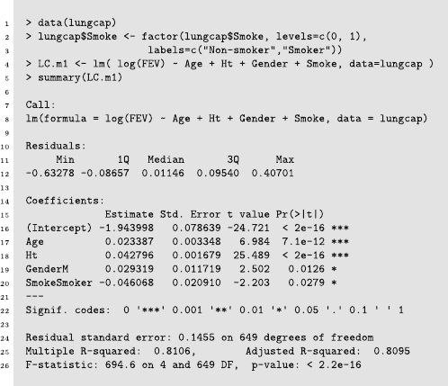
2.6 Fitting Linear Regression Models Using R 51
Fig. 2.6 The output of the summary() command after using lm() for the lungcap data
Each of these components can be accessed directly using constructs like, for
example, LC.m1$coefficients. However, most of the useful information is
accessed using r functions, such as coef(LC.m1), as demonstrated below.
These functions are discussed throughout this chapter, and are summarized
in Sect. 2.14. A summary of the information contained in the LC.m1 object
is displayed using the summary() command (Fig. 2.6). Most of this output is
explained in later sections, which refer back to the output in Fig. 2.6.
For now, observe that the parameter estimates are shown in the table in the
middle of the output (starting from line 14), in the column labelled Estimate.
The estimated standard errors appear in the column labelled Std. Error.
The parameter estimates are explicitly obtained using:
> coef( LC.m1 )
(Intercept) Age Ht GenderM SmokeSmoker
-1.94399818 0.02338721 0.04279579 0.02931936 -0.04606754
The estimate of σ is:
> summary( LC.m1 )$sigma
[1] 0.1454686
This information (as well as the residual degrees of freedom) appears in line 24
of the output shown in Fig. 2.6.
52 2 Linear Regression Models
2.7 Interpreting the Regression Coefficients
After fitting a model, interpretation of the model is strongly encouraged to
determine if the model makes physical sense, and to understand the story the
model is telling (Sect. 1.7).
The systematic component of linear regression model fitted to the gestation
data (Example 2.14)is
ˆμ = −2.678 + 0.1538x,
where μ =E[y], where y is the mean birthweight (in kg), and x is the gesta-
tional age in weeks. This model indicates that the mean birthweight increases
by approximately 0.1538 kg for each extra week of gestation, on average, over
the range of the data. The random component implies that the variation of
the weights around μ is approximately constant with s
2
=0.6010.
The interpretation for the systematic component model fitted to the lung
capacity data (Example 2.15) is different, because the response variable is
log(fev). This means that the systematic component is
μ = E[log(fev)]
= −1.944 + 0.02339x
1
+0.04280x
2
+0.02932x
3
− 0.04607x
4
(2.23)
for Age x
1
, Ht x
2
, the dummy variable for Gender x
3
and the dummy vari-
able for Smoke x
4
. The regression coefficients can only be interpreted for
their impact on μ = E[log(fev)] and not on E[fev] directly. However, since
E[log y] ≈ log E[y] = log μ (Problem 2.11), then (2.23) can be written as
log μ = log E[fev]
≈−1.944 + 0.02339x
1
+0.04280x
2
+0.02932x
3
− 0.04607x
4
. (2.24)
Now the parameter estimates can be used to approximately interpret the
effects of the explanatory variables on μ =E[fev] directly. For example, an
increase in height x
2
of one inch is associated with an increase in the mean
fev by a factor of exp(0.04280) = 1.044, assuming all other variables are
kept constant.
Parameter estimates for qualitative explanatory variables indicate how
much the value of μ changes compared to the reference level (after adjusting
for the effect of other variables), provided treatment coding is used (Sect. 1.4).
For the systematic component in (2.24), the value of μ will change by a factor
of exp(−0.04607) = 0.9550 for smokers (Smoke=1) compared to non-smokers
(Smoke=0). In other words, fev is likely to be a factor of 0.9550 lower for
smokers, assuming all other variables are kept constant.
The random component of the model (Example 2.15) indicates the vari-
ation of log(fev) around μ = E[log(fev)] is approximately constant, with
s
2
=0.02116.
2.8 Inference for Linear Regression Models: t-Tests 53
Interpreting the effects of correlated covariates is subtle. For example, in
the lung capacity data, height and age are positively correlated (Sect. 1.7).
Height generally increases with age for youth, so the effect on fev of increas-
ing age for fixed height is not the same as the overall increase in fev as age
increases. The overall increase in fev would reflect the combined effects of
height and age as both increase. The coefficient in the linear model reflects
only the net effect of a covariate, eliminating any concomitant changes in the
other covariates that might normally be present if all the covariate varied in
an uncontrolled fashion.
Also, note that the data are observational, so no cause-and-effect conclu-
sion is implied (Sect. 1.7).
2.8 Inference for Linear Regression Models: t-Tests
2.8.1 Normal Linear Regression Models
Up to now, no specific statistical distribution has been assumed for the re-
sponses in the regression. The responses have simply been assumed to be
independent and to have constant variance. However, to undertake formal
statistical inference we need to be more specific. The usual assumption of lin-
ear regression is that the responses are normally distributed, either with con-
stant variance or with variances that are proportional to the known weights.
This can be stated as:
⎧
⎪
⎨
⎪
⎩
y
i
∼ N(μ
i
,σ
2
/w
i
)
μ
i
= β
0
+
p
j=1
β
j
x
ji
.
(2.25)
Model (2.25) is called a normal linear regression model. Under the assump-
tions of this model, hypothesis tests and confidence intervals can be devel-
oped. In practice, the assumption of normality is not as crucial is it might
appear, as most of the tests we will develop remain valid for large n even
when the responses are not normally distributed. The main significance of
the normality therefore is to develop tests and confidence intervals that are
valid for small sample sizes.
2.8.2 The Distribution of
ˆ
β
j
Expressions for computing estimates of var[
ˆ
β
j
] were given in Sects. 2.3.4
and 2.5.4. When a normal linear regression model (2.25) is adopted, the entire
distributions of the regression parameters are known, not just the variance.
Using Model (2.25), the
ˆ
β
j
are random variables which follow normal distri-

54 2 Linear Regression Models
butions, since
ˆ
β
j
is a linear combination of the y
i
(Sect. 2.5.2). Specifically,
for normal linear regression models,
ˆ
β
j
∼ N(β
j
, var[
ˆ
β
j
]). (2.26)
This means that
ˆ
β
j
has a normal distribution with mean β
j
and variance
var[
ˆ
β
j
]. Note that var[
ˆ
β
j
] is a product of σ (approximately inversely propor-
tional to
√
n ) and the known values of the explanatory variable and weights.
From (2.26),
Z =
ˆ
β
j
− β
j
se(
ˆ
β
j
)
,
where se(
ˆ
β
j
)=
var[
ˆ
β
j
], and Z has a standard normal distribution when σ
2
is known. When σ
2
is unknown, estimate σ
2
by s
2
and hence estimate var[
ˆ
β
j
]
by var[
ˆ
β
j
]. Then
T =
ˆ
β
j
− β
j
se(
ˆ
β
j
)
has a Student’s t distribution with n −p
degrees of freedom, where se(
ˆ
β
j
)=
var[
ˆ
β
j
]. Note that Student’s t-distribution converges to the standard nor-
mal as the degrees of freedom increase.
2.8.3 Hypothesis Tests for β
j
Consider testing the null hypothesis H
0
: β
j
= β
0
j
against a one-sided alterna-
tive (H
A
: β
j
>β
0
j
or H
A
: β
j
<β
0
j
) or a two-sided alternative (H
A
: β
j
= β
0
j
),
where β
0
j
is some hypothesized value of β
j
(usually zero). The statistic
T =
ˆ
β
j
− β
0
j
se(
ˆ
β
j
)
(2.27)
is used to test this hypothesis. When H
0
is true, T has a t-distribution with
n − p
degrees of freedom when σ
2
is unknown, so we determine significance
by referring to this distribution.
Each individual t-test determines whether evidence exists that the param-
eter is statistically significantly different from β
0
j
in the presence of the other
variables currently in the model.
Example 2.16. After fitting Model (2.22) to the lung capacity data in r (data
set: lungcap), the output of the summary() command in Fig. 2.6 (p. 51)
reports information about the parameter estimates in the table in the centre
of the output (starting from line 14):
2.8 Inference for Linear Regression Models: t-Tests 55
•theEstimate column contains the parameter estimates
ˆ
β
j
;
•the Std. Error column contains the corresponding standard errors
se(
ˆ
β
j
);
•thet value column contains the corresponding t-statistic (2.27) for test-
ing H
0
: β
j
=0;
•thePr(>|t|) column contains the corresponding two-tailed P -values for
the hypothesis tests. (The one-tailed P -value is the two-tailed P -value
divided by two.)
Line 22 in Fig. 2.6 (p. 51) regarding Signif. codes needs explanation. The
*** indicates a two-tailed P-value between 0 and 0.001; ** indicates a two-
tailed P -value between 0.001 and 0.01; * indicates a two-tailed P -value be-
tween 0.01 and 0.05; . indicates a two-tailed P-value between 0.05 and 0.10.
This information can be accessed directly using coef(summary()):
> round(coef( summary( LC.m1 ) ), 5)
Estimate Std. Error t value Pr(>|t|)
(Intercept) -1.94400 0.07864 -24.72067 0.00000
Age 0.02339 0.00335 6.98449 0.00000
Ht 0.04280 0.00168 25.48933 0.00000
GenderM 0.02932 0.01172 2.50196 0.01260
SmokeSmoker -0.04607 0.02091 -2.20311 0.02794
For example, consider a hypothesis test for β
4
(the coefficient for Smoke). To
test H
0
: β
4
= 0 against the alternative H
A
: β
4
= 0 (in the presence of age,
height and gender), the output shows that the t-score is t = −2.203, and
the corresponding two-tailed P -value is 0.02794. Thus, some evidence exists
that smoking status is statistically significant when age, height and gender
are in the model. If gender was omitted from the model and the relevant
null hypothesis retested, the test has a different meaning: this second test
determines if age is significant in the model adjusted only for height (but not
gender). Consequently, we should expect the test statistic and P -values to be
different, and so the conclusion may differ also.
2.8.4 Confidence Intervals for β
j
While hypothesis tests are useful for detecting statistical significance, often
the size of the effect is of greater interest. This can be estimated by computing
confidence intervals. The estimates
ˆ
β
j
and the corresponding standard errors
se(
ˆ
β
j
) can be used to form 100(1−α)% confidence intervals for each estimate
using
ˆ
β
j
± t
∗
α/2,n−p
se(
ˆ
β
j
),
where t
∗
α/2,n−p
is the value such that an area α/2 is in each tail of the t-
distribution with n −p
degrees of freedom. Rather than explicitly using the

56 2 Linear Regression Models
formula, confidence intervals are found in r using the confint() command.
By default, 95% confidence intervals are produced; other levels are produced
by using, for example, level=0.90 in the call to confint().
Example 2.17. For the lung capacity data (data set: lungcap), find the 95%
confidence interval for all five regression coefficients in model LC.m1 using
confint():
> confint( LC.m1 )
2.5 % 97.5 %
(Intercept) -2.098414941 -1.789581413
Age 0.016812109 0.029962319
Ht 0.039498923 0.046092655
GenderM 0.006308481 0.052330236
SmokeSmoker -0.087127344 -0.005007728
For example, the 95% confidence interval for β
4
is from −0.08713 to
−0.005008.
2.8.5 Confidence Intervals for μ
The fitted values ˆμ are used to estimate the mean value for given values
of the explanatory variables. Using the expressions for computing var[ˆμ
g
]
(Sect. 2.3.5; Sect. 2.5.5), the 100(1 − α)% confidence interval for the fitted
value is
ˆμ
g
± t
∗
α/2,n−p
se(ˆμ),
where se(ˆμ
g
)=
var[ ˆμ
g
], and where t
∗
α/2,n−p
is the value such that an area
α/2 is in each tail of the t-distribution with n−p
degrees of freedom. Rather
than explicitly using the formulae, r returns the standard errors when making
predictions using predict() with the input se.fit=TRUE, from which the
confidence intervals can be formed.
Example 2.18. For the lung capacity data (data set: lungcap), suppose we
wish to estimate μ = E[log(fev)] for female smokers aged 18 who are 66
inches tall. Using r, we first create a new data frame containing the values
of the explanatory variables for which we need to make the prediction:
> new.df <- data.frame(Age=18, Ht=66, Gender="F", Smoke="Smoker")
Then, use predict() to compute the estimates of μ:
> out <- predict( LC.m1, newdata=new.df, se.fit=TRUE)
> names(out)
[1] "fit" "se.fit" "df" "residual.scale"
> out$se.fit
[1] 0.02350644
2.8 Inference for Linear Regression Models: t-Tests 57
> tstar <- qt(df=LC.m1$df, p=0.975 ) # For a 95% CI
> ci.lo <- out$fit - tstar*out$se.fit
> ci.hi <- out$fit + tstar*out$se.fit
> CIinfo <- cbind( Lower=ci.lo, Estimate=out$fit, Upper=ci.hi)
> CIinfo
Lower Estimate Upper
1 1.209268 1.255426 1.301584
The prediction is ˆμ =1.255, and the 95% confidence interval is from 1.209 to
1.302. Based on the discussion in Sect. 2.7, an approximate confidence interval
for E[fev]is
> exp(CIinfo)
Lower Estimate Upper
1 3.351032 3.509334 3.675114
This idea can be extended to compute the confidence intervals for 18 year-
old female smokers for varying heights:
> newHt <- seq(min(lungcap$Ht), max(lungcap$Ht), by=2)
> newlogFEV <- predict( LC.m1, se.fit=TRUE,
newdata=data.frame(Age=18, Ht=newHt, Gender="F", Smoke="Smoker"))
> ci.lo <- exp( newlogFEV$fit - tstar*newlogFEV$se.fit )
> ci.hi <- exp( newlogFEV$fit + tstar*newlogFEV$se.fit )
Notice that the intervals do not have the same width over the whole range
of the data:
> cbind( Ht=newHt, FEVhat=exp(newlogFEV$fit), SE=newlogFEV$se.fit,
Lower=ci.lo, Upper=ci.hi, CI.Width=ci.hi - ci.lo)
Ht FEVhat SE Lower Upper CI.Width
1 46 1.491095 0.04886534 1.354669 1.641259 0.2865900
2 48 1.624341 0.04585644 1.484469 1.777392 0.2929226
3 50 1.769494 0.04289937 1.626540 1.925011 0.2984711
4 52 1.927618 0.04000563 1.781987 2.085151 0.3031639
5 54 2.099873 0.03719000 1.951990 2.258959 0.3069685
6 56 2.287520 0.03447163 2.137804 2.447722 0.3099183
7 58 2.491936 0.03187542 2.340743 2.652894 0.3121513
8 60 2.714619 0.02943370 2.562170 2.876138 0.3139672
9 62 2.957201 0.02718813 2.803464 3.119368 0.3159041
10 64 3.221460 0.02519123 3.065984 3.384820 0.3188364
11 66 3.509334 0.02350644 3.351032 3.675114 0.3240817
12 68 3.822932 0.02220493 3.659826 3.993308 0.3334820
13 70 4.164555 0.02135689 3.993518 4.342917 0.3493998
14 72 4.536705 0.02101728 4.353286 4.727852 0.3745665
15 74 4.942111 0.02121053 4.740502 5.152294 0.4117924
58 2 Linear Regression Models
2.9 Analysis of Variance for Regression Models
A linear regression model, having been fitted to the data by least squares,
yields a fitted value
ˆμ
i
=
ˆ
β
0
+
p
j=1
x
ij
ˆ
β
j
for each observation y
i
. Each observation therefore can be separated into a
component predicted by the model, and the remainder or residual that is left
over, as
y
i
=ˆμ
i
+(y
i
− ˆμ
i
).
In other words, Data = Fit + Residual.
The simplest possible regression model is that with p = 0 and no covari-
ates x
ij
.Inthatcaseˆμ =
ˆ
β
0
=¯y
w
, where ¯y
w
=
n
i=1
w
i
y
i
/
n
i=1
w
i
is the
weighted mean of the observations. In order to evaluate the contribution of
the covariates x
ij
, it is more useful to consider the corresponding decompo-
sition of the mean-corrected data,
y
i
− ¯y
w
=(ˆμ
i
− ¯y
w
)+(y
i
− ˆμ
i
).
Squaring each of these terms and summing them over i leads to the key
identity
sst = ssReg + rss
where sst =
n
i=1
w
i
(y
i
− ¯y
w
)
2
is the total sum of squares, ssReg =
n
i=1
w
i
(ˆμ
i
− ¯y
w
)
2
is the regression sum of squares,andrss =
n
i=1
w
i
(y
i
−
ˆμ
i
)
2
is the residual sum of squares. The cross-product terms (ˆμ
i
−¯y
w
)(y
i
−ˆμ
i
)
sum to zero, and so don’t appear in this identity. The identity embodies the
principle that variation in the response variable comes from two sources:
firstly a systematic component that can be attributed to changes in the ex-
planatory variables (ssReg), and secondly a random component that cannot
be predicted (rss). This identity is the basis of what is called analysis of
variance, because it analyses the sources from which variance in the data
arises.
It is of key interest to know whether the explanatory variables are useful
predictors of the responses. This question can be answered statistically by
testing whether the regression sum of squares ssReg is larger than would be
expected due to random variation; in other words, whether ssReg is large
relative to rss after taking the number of explanatory variables into account.
The null hypothesis is the assertion that β
j
= 0 for all j =1,...,p.To
develop such a test, first note that rss/σ
2
has a chi-square distribution with
n − p
degrees of freedom, for a normal linear regression model. Likewise,
under the null hypothesis, it can be shown that ssReg/σ
2
has a chi-square

2.9 Analysis of Variance for Regression Models 59
Tabl e 2 .2 The general form of an analysis of variance table for a linear regression model
(Sect. 2.9)
Source of variation Sums of squares df Mean square F
Systematic component ssReg p
− 1 msReg =
ssReg
p
− 1
F =
msReg
mse
Random component rss n − p
mse =
rss
n − p
= s
2
Total variation sst n − 1
distribution with p
− 1 degrees of freedom for a normal linear regression
model. This means that the ratio
F =
ssReg/(p
− 1)
rss/(n − p
)
=
msReg
mse
(2.28)
follows an F -distribution with (p
− 1,n− p
) degrees of freedom. The mse,
the mean-square error, is equal to s
2
, the unbiased estimator of σ
2
that we
have previously seen. msReg is the mean-square for the regression.
A large value for F means that the proportion of the variation that can be
explained by the systematic component is large relative to s
2
; a small value
for F means that the proportion of the variation that can be explained by
the systematic component is small relative to s
2
.
The computations are conveniently arranged in an analysis of variance
(anova) table (Table 2.2).
The r summary() command does not show the details of the anova ta-
ble (Fig. 2.6,p.51), but the results are reported in the final line of output
(line 26): the F -statistic is labelled F-statistic, followed by the correspond-
ing degrees of freedom (labelled DF), and the P -value for the test (labelled
p-value). The F -statistic and the corresponding degrees of freedom are re-
turned using summary(LC.m1)$fstatistic. There is also an anova() func-
tion that is demonstrated in the next section.
The proportion of the total variation explained by the regression is the
coefficient of determination,
R
2
=
ssReg
sst
=1−
rss
sst
. (2.29)
Clearly, by the definition, R
2
is bounded between zero and one. R
2
is some-
times also called multiple R
2
, because it is equal to the squared Pearson cor-
relation coefficient between the y
i
and the fitted values ˆμ
i
, using the weights
w
i
. r reports the value of R
2
in the model summary(), as shown in Fig. 2.6
(p. 51), where R
2
is labelled Multiple R-squared on line 25.

60 2 Linear Regression Models
Adding a new explanatory variable to the regression model cannot increase
rss and hence R
2
tends to increase with the size p of the model even if the
explanatory variables have no real explanatory power. For this reason, some
statisticians like to adjust R
2
for the number of explanatory variables in the
model. The adjusted R
2
, denoted
¯
R
2
, is defined by
¯
R
2
=1−
rss/(n − p
)
sst/(n − 1)
=1− (1 −R
2
)
n − 1
n − p
.
It can be seen that 1 −
¯
R
2
is the ratio of the residual to the total in the mean
square column of the anova table, whereas 1 −R
2
is the corresponding ratio
for the sums of squares column. However
¯
R
2
is not the ratio of msReg to
sst/(n − 1), because the entries is the mean square column do not sum.
Unlike R
2
,
¯
R
2
may be negative. This occurs whenever msReg < mse,which
can be taken to indicate a very poor model. In the model summary() (Fig. 2.6,
p. 51), r reports
¯
R
2
, called Adjusted R-squared. F and R
2
are closely
related quantities (Problem 2.8), but it is F that is used to formally test
whether the regression is statistically significant.
Example 2.19. For the lung capacity data (data set: lungcap), and
Model (2.22) with age, height, gender and smoking status as explanatory
variables, compute rss and sst (recalling that y = log(FEV)):
> mu <- fitted( LC.m1 ); RSS <- sum( (y - mu)^2 )
> SST <- sum( (y - mean(y) )^2 )
> c(RSS=RSS, SST=SST, SSReg = SST-RSS)
RSS SST SSReg
13.73356 72.52591 58.79236
> R2 <- 1 - RSS/SST # Compute R2 explicitly
> c( "Output R2" = summary(LC.m1)$r.squared, "Computed R2" = R2,
"adj R2" = summary(LC.m1)$adj.r.squared)
Output R2 Computed R2 adj R2
0.8106393 0.8106393 0.8094722
The analysis of variance table (Table 2.3) compiles the necessary information.
Compare these results to the output of summary(LC.m1) in Fig. 2.6 (p. 51).
The summary of the F -test, which includes the numerator and denominator
degree of freedom, is
> summary(LC.m1)$fstatistic
value numdf dendf
694.5804 4.0000 649.0000

2.10 Comparing Nested Models 61
Tabl e 2 .3 The anova table for Model (2.22) fitted to the lung capacity data, parti-
tioning the total sum-of-squares into components due to the systematic and random
components (Example 2.19)
Source ss df ms F
Systematic component 58.79 4 14.70 694.6
Random component 13.73 649 0.02116
Total variation 72.53 653
2.10 Comparing Nested Models
2.10.1 Analysis of Variance to Compare Two Nested
Models
Rather than evaluating a single model, a researcher may wish to compare
two models. First consider comparing two nested linear regression models.
Model A is nested in Model B if Model A can be obtained from Model B by
setting some parameter(s) in Model B to zero or, more generally, if Model A is
a special case of Model B. For example, for the lung capacity data a researcher
may wish to compare two models with the systematic components
Model A: μ
A
= β
0
+ β
1
x
1
+ β
4
x
4
;
Model B: μ
B
= β
0
+ β
1
x
1
+ β
2
x
2
+ β
3
x
3
+ β
4
x
4
.
Model A is nested in Model B, since Model A is a special case of Model B
obtained by setting β
2
= β
3
=0.
In comparing these models, we wish to know whether the more complex
Model B is necessary, or whether the simpler Model A will suffice. Formally,
the null hypothesis is that the two models are equivalent, so that we test H
0
:
β
2
= β
3
= 0 against the alternative that β
2
and β
3
are not both zero.
Consider using the lungcap data frame, and fitting the two models:
> LC.A <- lm( log(FEV) ~ Age + Smoke, data=lungcap )
> LC.B <- lm( log(FEV) ~ Age + Ht + Gender + Smoke, data=lungcap )
Now compute the respective rss:
> RSS.A <- sum( resid(LC.A)^2 ) # resid() computes residuals
> RSS.B <- sum( resid(LC.B)^2 )
> c( ModelA=RSS.A, ModelB=RSS.B)
ModelA ModelB
28.91982 13.73356
62 2 Linear Regression Models
The difference between the values of rss is called the sum-of-squares (or ss):
> SS <- RSS.A - RSS.B; SS
[1] 15.18626
> DF <- df.residual(LC.A) - df.residual(LC.B); DF
[1] 2
The ss measures the reduction in the rss gained by using the more complex
Model B. This reduction in rss is associated with an increase of two degrees
of freedom. Is this reduction statistically significant?
The formal test requires comparing the ss divided by the change in the
degrees of freedom, to the rss for Model B divided by the degrees of freedom
for Model B:
> df.B <- df.residual(LC.B); df.B
[1] 649
> Fstat <- (SS/DF) / ( RSS.B/df.B ); Fstat
[1] 358.8249
A P -value is found by comparing to an F -distribution with (2, 649) degrees
of freedom:
> pf(Fstat, df1=DF, df2=df.B, lower.tail=FALSE)
[1] 1.128849e-105
The P -value is almost zero, providing strong evidence that Model B is signif-
icantly different from Model A. In r, the results are displayed using anova():
> anova( LC.A, LC.B )
Analysis of Variance Table
Model 1: log(FEV) ~ Age + Smoke
Model 2: log(FEV) ~ Age + Ht + Gender + Smoke
Res.Df RSS Df Sum of Sq F Pr(>F)
1 651 28.920
2 649 13.734 2 15.186 358.82 < 2.2e-16 ***
---
Signif. codes: 0 '***' 0.001 '**' 0.01 '*' 0.05 '.' 0.1''1
More generally, consider fitting two nested models, say Model A and
Model B, with systematic components
Model A: ˆμ
A
= β
0
+ β
1
x
1
+ ···+ β
p
A
x
p
A
Model B: ˆμ
B
= β
0
+ β
1
x
1
+ ···+ β
p
A
x
p
A
+ ···+ β
p
B
x
p
B
.
Model A is nested in Model B, because Model A is obtained by setting
β
p
A
+1
,...,β
p
B
= 0 in Model B. The difference between the rss computed
for each model is the ss due to the difference between the models, based
on p
B
− p
A
degrees of freedom. Assuming H
0
: β
p
A
+1
= ··· = β
p
B
=0is

2.10 Comparing Nested Models 63
true, the models are identical and ss is equivalent to residual variation. The
test-statistic is
F =
(rss
A
− rss
B
)/(p
B
− p
A
)
s
2
=
ss
B
/(p
B
− p
A
)
rss
B
/(n − p
B
)
. (2.30)
A P -value is deduced by referring to an F -distribution with (p
B
−p
A
,n−p
B
)
degrees of freedom.
2.10.2 Sequential Analysis of Variance
The analysis of variance table just described is useful for comparing any two
nested models. Commonly, a sequence of nested models is compared. For each
pair of nested models in the sequence, the change in the rss (the ) and the
corresponding change in the degrees of freedom are recorded and organised
in a table.
As an example, consider model LC.B fitted to the lungcap data
(Sect. 2.10.1,p.61), which explores the relationship between FEV and Smoke,
with the extraneous variables Age, Ht and Gender. A sequence of nested
models could be compared:
> LC.0 <- lm( log(FEV) ~ 1, data=lungcap) # No explanatory variables
> LC.1 <- update(LC.0,.~.+Age) # Age
> LC.2 <- update(LC.1,.~.+Ht) #AgeandHeight
> LC.3 <- update(LC.2,.~.+Gender) # Age, Height and Gender
> LC.4 <- update(LC.3,.~.+Smoke) # Then, add smoking status
Notice the use of update() to update models. To update model LC.0 to form
model LC.1, specify which components of LC.0 should be changed. The first
input is the model to be changed, and the second is the component of the
model specification to change. Here we wish to change the formula given in
LC.0. The left-hand side of the formula remains the same (as specified by .)
but the original right-hand side (indicated by .)hasAge added. Of course,
LC.1 could be also specified directly.
The rss can be computed for each model:
> RSS.0 <- sum( resid(LC.0)^2 )
> RSS.1 <- sum( resid(LC.1)^2 )
> RSS.2 <- sum( resid(LC.2)^2 )
> RSS.3 <- sum( resid(LC.3)^2 )
> RSS.4 <- sum( resid(LC.4)^2 )
> RSS.list <- c( Model4=RSS.4, Model3=RSS.3, Model2=RSS.2,
Model1=RSS.1, Model0=RSS.0)
> RSS.list
Model4 Model3 Model2 Model1 Model0
13.73356 13.83627 13.98958 29.31586 72.52591
64 2 Linear Regression Models
Notice that the rss reduces as the models become more complex. The change
in the rss,thess, can also be computed:
> SS.list <- diff(RSS.list); SS.list
Model3 Model2 Model1 Model0
0.1027098 0.1533136 15.3262790 43.2100549
The changes in the degrees of freedom between these nested models are all one
in this example. As before, we compare these changes in rss to an estimate
of σ
2
= mse, using the F -statistic (2.30):
> s2 <- summary(LC.4)$sigma^2 # One way to get MSE
> F.list <- (SS.list / 1) / s2; F.list
Model3 Model2 Model1 Model0
4.853708 7.245064 724.266452 2041.956379
> P.list <- pf( F.list, 1, df.residual(LC.4), lower.tail=FALSE)
> round(P.list, 6)
Model3 Model2 Model1 Model0
0.027937 0.007293 0.000000 0.000000
These computations are all performed in r by using anova(), and providing
as input the final model in the set of nested models:
> anova(LC.4)
Analysis of Variance Table
Response: log(FEV)
Df Sum Sq Mean Sq F value Pr(>F)
Age 1 43.210 43.210 2041.9564 < 2.2e-16 ***
Ht 1 15.326 15.326 724.2665 < 2.2e-16 ***
Gender 1 0.153 0.153 7.2451 0.007293 **
Smoke 1 0.103 0.103 4.8537 0.027937 *
Residuals 649 13.734 0.021
---
Signif. codes: 0 '***' 0.001 '**' 0.01 '*' 0.05 '.' 0.1''1
The F -values and P -values are the same as those found in the calculations
above.
This discussion shows that a series of sequential tests is performed. The
last formally tests if Smoke is significant in the model, given that Age, Ht
and Gender are already in the model. In other words, the F-test for Smoke
adjusts for Age, Ht and Gender. In general, the F -tests in sequential anova
tables are always adjusted for all previous terms in the model.
Because the F -tests are adjusted for other terms in the model, numerous
F -tests are possible to test for the effect of Smoke, depending on the order
in which the corresponding nested models are compared. For example, tests
based on Smoke include:
•TestforSmoke without adjusting for any other explanatory variables;
•TestforSmoke after first adjusting for Age;
•TestforSmoke after first adjusting for Ht;
•TestforSmoke after first adjusting for both Age and Gender.

2.10 Comparing Nested Models 65
These tests consider different hypotheses regarding Smoke so may produce
different results. In contrast, t-tests (Sect. 2.8.3) present the same information
after all explanatory variables are in the model whatever order the variables
are added, as t-tests are adjusted for all other variables in the final model.
Because the t-tests of Sect. 2.8.3 always adjust for all other terms in the
model, the results from the t-andF -tests are generally different. However
the final F -test in a sequential anova table, if it is on 1 degree of freedom,
is equivalent to the corresponding two-sided t-test. For example, the P -value
for Smoke in the above anova table (P =0.0279) is the same as the P -value
for Smoke given in Sect. 2.8.3, and the F -statistic for Smoke is the square of
the t-statistic for Smoke. In general, the square of a t-statistic on ν degrees of
freedom yields an F -statistic on (1,ν) degrees of freedom, so any two-sided
t-test can be expressed as an F-test.
The anova table shows the results of F -tests for the variables in the
presented order. The models higher in the table are special cases of the models
lower in the table (that is, models higher in the table are nested within models
lower in the table). The order in which the explanatory variables are fitted is
important, except in very special cases (usually in an experiment explicitly
designed to ensure the order of fitting is not important).
More generally, testing a series of sequential models is equivalent to sep-
arating the systematic component into contributions from each explanatory
variable (Table 2.4).
Example 2.20. Model LC.4 (in Sect. 2.10.2) fits the explanatory variables Age,
Ht, Gender and Smoke in that order (data set: lungcap
). Consider fitting the
explanatory variables in reverse order:
> LC.4.rev <- lm(log(FEV) ~ Smoke + Gender + Ht + Age, data=lungcap)
> anova(LC.4.rev)
Tabl e 2 . 4 The general form of an analysis of variance table for a normal linear re-
gression model, separating the systematic component into the contributions for each
explanatory variable (Sect. 2.10.2)
Mean
Source of variation ss df square F
⎧
⎪
⎪
⎪
⎪
⎪
⎪
⎪
⎪
⎪
⎨
⎪
⎪
⎪
⎪
⎪
⎪
⎪
⎪
⎪
⎩
Due to x
1
ss(x
1
)df
1
ms
1
ms
1
mse
Due to x
2
(adjusted for x
1
) ss(x
2
|x
1
)df
2
ms
2
ms
2
mse
Due to x
3
(adjusted for x
1
and x
2
) ss(x
3
|x
1
,x
2
)df
3
ms
3
ms
3
mse
.
.
.
.
.
.
.
.
.
.
.
.
.
.
.
Due to x
p
(adjusted for x
1
,...,x
p−1
) ss(x
p
|x
1
,...,x
p−1
)df
p
ms
p
ms
p
mse
Due to randomness rss n − p
mse
Total variation sst n − 1
66 2 Linear Regression Models
Analysis of Variance Table
Response: log(FEV)
Df Sum Sq Mean Sq F value Pr(>F)
Smoke 1 4.334 4.334 204.790 < 2.2e-16 ***
Gender 1 2.582 2.582 122.004 < 2.2e-16 ***
Ht 1 50.845 50.845 2402.745 < 2.2e-16 ***
Age 1 1.032 1.032 48.783 7.096e-12 ***
Residuals 649 13.734 0.021
---
Signif. codes: 0 '***' 0.001 '**' 0.01 '*' 0.05 '.' 0.1''1
The level of significance of Smoke depends on whether this variable is added
first (model LC.4) or last, after adjusting for Age, Ht and Gender. Sometimes,
a variable may be significant when added first, but not at all significant when
added after other variables. Thus the effect of a variable may depend on
whether or not the model is adjusted for other variables.
2.10.3 Parallel and Independent Regressions
Section 2.10.1 discussed the general case of testing any two nested models. We
now discuss a particular set of nested models that are commonly compared,
using the lung capacity data lungcap. For simplicity, we consider the case of
one covariate (height x
2
) and one factor (smoking status x
4
) to fix ideas.
A naive (and obviously untrue) model is that μ = E[log(fev)] does not
depend on smoking status or height (Fig. 2.7,p.68, top left panel). The fitted
systematic component is
ˆμ =0.9154, (2.31)
with rss =72.53 on 653 degrees of freedom. Note that this model simply
estimates the mean value of y = log(fev):
> mean(log(lungcap$FEV))
[1] 0.915437
To consider if the influence of height x
2
on μ = E[log(fev)] is significant,
the fitted model is (Fig. 2.7, top right panel)
ˆμ = −2.271 + 0.05212x
2
, (2.32)
with rss =14.82 on 652 degrees of freedom. This regression model does not
differentiate between smokers and non-smokers. Is the relationship different
for smokers and non-smokers?
To consider this, add smoking status x
4
as an explanatory variable
(Fig. 2.7, bottom left panel):
ˆμ = −2.277 + 0.05222x
2
− 0.006830x
4
, (2.33)

2.10 Comparing Nested Models 67
with rss =14.82 on 651 degrees of freedom, and where x
4
= 0 refers to non-
smokers and x
4
= 1 to smokers. Using (2.33), the two separate systematic
components are
ˆμ =
−2.277 + 0.05222x
2
for non-smokers (set x
4
=0)
−2.284 + 0.05222x
2
for smokers (set x
4
=1)
with different intercepts. Model (2.33) produces two parallel regression lines;
only the intercepts differ but are so similar than the two lines can hardy be
distinguished on the plot (Fig. 2.7, bottom left panel). This model assumes
two separate systematic components, but a common random component and
so a common estimate of σ
2
.
Notice that the regression equation intercepts for smokers and non-smokers
are the same if the coefficient for x
4
is zero. Hence, to formally test if the
intercepts are different, a test of the corresponding β is conducted. In r:
> printCoefmat(coef(summary(lm( log(FEV) ~ Ht + Smoke, data=lungcap))))
Estimate Std. Error t value Pr(>|t|)
(Intercept) -2.2767801 0.0656677 -34.6712 <2e-16 ***
Ht 0.0522196 0.0010785 48.4174 <2e-16 ***
SmokeSmoker -0.0068303 0.0205450 -0.3325 0.7397
---
Signif. codes: 0 '***' 0.001 '**' 0.01 '*' 0.05 '.' 0.1''1
The evidence suggests that different intercepts are not needed when the slopes
of the lines are common. This is not unexpected given Fig. 2.7.
Perhaps the relationships between μ = E[log(fev)] and height have differ-
ent intercepts and slopes for smokers and non-smokers also (Fig 2.7, bottom
right panel). Different slopes can be modelled using the interaction between
height and smoking status as an explanatory variable:
ˆμ = −2.281 + 0.05230x
2
− 0.002294x
4
+
interaction
0.002294x
2
.x
4
, (2.34)
with rss =14.82 on 650 degrees of freedom. Model (2.34) produces two sep-
arate systematic components; both the intercepts and slopes differ (Fig. 2.7,
bottom right panel):
ˆμ =
−2.281 + 0.05230x
2
for non-smokers (set x
4
=0)
−2.137 + 0.05000x
2
for smokers (set x
4
=1).
This is not equivalent to fitting two separate linear regression models, since
the same estimate of σ
2
is shared by both systematic components.
Notice that the regression equation slopes for smokers and non-smokers
are the same if the coefficient for the interaction between x
2
and x
4
is zero.
Hence, to formally test if the slopes are different, a test of the corresponding

45 50 55 60 65 70 75
0.0
0.5
1.0
1.5
Constant term only
Height (cm)
log(FEV, in litres)
l
l
l
l
l
l
l
l
l
l
l
l
l
l
l
l
l
l
l
l
l
l
l
l
l
l
l
l
l
l
l
l
l
l
l
l
l
l
l
l
l
l
l
l
l
l
l
l
l
l
l
l
l
l
l
l
l
l
l
l
l
l
l
l
l
l
l
l
l
l
l
l
l
l
l
l
l
l
l
l
l
l
l
l
l
l
l
l
l
l
l
l
l
l
l
l
l
l
l
l
l
l
l
l
l
l
l
l
l
l
l
l
l
l
l
l
l
l
l
l
l
l
l
l
l
l
l
l
l
l
l
l
l
l
l
l
l
l
l
l
l
l
l
l
l
l
l
l
l
l
l
l
l
l
l
l
l
l
l
l
l
l
l
l
l
l
l
l
l
l
l
l
l
l
l
l
l
l
l
l
l
l
l
l
l
l
l
l
l
l
l
l
l
l
l
l
l
l
l
l
l
l
l
l
l
l
l
l
l
l
l
l
l
l
l
l
l
l
l
l
l
l
l
l
l
l
l
l
l
l
l
l
l
l
l
l
l
l
l
l
l
l
l
l
l
l
l
l
l
l
l
l
l
l
l
l
l
l
l
l
l
l
l
l
l
l
l
l
l
l
l
l
l
l
l
l
l
l
l
l
l
l
l
l
l
l
l
l
l
l
l
l
l
l
l
l
l
l
l
l
l
l
l
l
l
l
l
l
l
l
l
l
l
l
l
l
l
l
l
l
l
l
l
l
l
l
l
l
l
l
l
l
l
l
l
l
l
l
l
l
l
l
l
l
l
l
l
l
l
l
l
l
l
l
l
l
l
l
l
l
l
l
l
l
l
l
l
l
l
l
l
l
ll
l
l
l
l
l
l
l
l
l
l
l
l
l
l
l
l
l
l
l
l
l
l
l
l
l
l
l
l
l
l
l
l
l
l
l
l
l
l
l
l
l
l
l
l
l
l
l
l
l
l
l
l
l
l
l
l
l
l
l
l
l
l
l
l
l
l
l
l
l
l
l
l
l
l
l
l
l
l
l
l
l
l
l
l
l
l
l
l
l
l
l
l
l
l
l
l
l
l
l
l
l
l
l
l
l
l
l
l
l
l
l
l
l
l
l
l
l
l
l
l
l
l
l
l
l
l
l
l
l
l
l
l
l
l
l
l
l
l
l
l
l
l
l
l
l
l
l
l
l
l
l
l
l
l
l
l
l
l
l
l
l
l
l
l
l
l
l
l
l
l
l
l
l
l
l
l
l
l
l
l
l
l
l
l
l
l
l
l
l
l
l
l
l
l
l
l
l
l
l
l
l
l
l
l
l
l
l
l
l
l
l
l
l
l
l
l
l
l
l
l
l
l
l
l
l
l
l
l
l
l
l
l
l
ll
l
l
l
l
l
l
l
l
l
l
l
l
l
l
l
l
l
l
l
l
l
l
l
l
l
l
l
l
l
l
l
l
l
l
l
l
l
l
l
l
l
l
l
l
l
l
l
Non−smokers
Smokers
45 50 55 60 65 70 75
0.0
0.5
1.0
1.5
Single model
Height (cm)
log(FEV, in litres)
l
l
l
l
l
l
l
l
l
l
l
l
l
l
l
l
l
l
l
l
l
l
l
l
l
l
l
l
l
l
l
l
l
l
l
l
l
l
l
l
l
l
l
l
l
l
l
l
l
l
l
l
l
l
l
l
l
l
l
l
l
l
l
l
l
l
l
l
l
l
l
l
l
l
l
l
l
l
l
l
l
l
l
l
l
l
l
l
l
l
l
l
l
l
l
l
l
l
l
l
l
l
l
l
l
l
l
l
l
l
l
l
l
l
l
l
l
l
l
l
l
l
l
l
l
l
l
l
l
l
l
l
l
l
l
l
l
l
l
l
l
l
l
l
l
l
l
l
l
l
l
l
l
l
l
l
l
l
l
l
l
l
l
l
l
l
l
l
l
l
l
l
l
l
l
l
l
l
l
l
l
l
l
l
l
l
l
l
l
l
l
l
l
l
l
l
l
l
l
l
l
l
l
l
l
l
l
l
l
l
l
l
l
l
l
l
l
l
l
l
l
l
l
l
l
l
l
l
l
l
l
l
l
l
l
l
l
l
l
l
l
l
l
l
l
l
l
l
l
l
l
l
l
l
l
l
l
l
l
l
l
l
l
l
l
l
l
l
l
l
l
l
l
l
l
l
l
l
l
l
l
l
l
l
l
l
l
l
l
l
l
l
l
l
l
l
l
l
l
l
l
l
l
l
l
l
l
l
l
l
l
l
l
l
l
l
l
l
l
l
l
l
l
l
l
l
l
l
l
l
l
l
l
l
l
l
l
l
l
l
l
l
l
l
l
l
l
l
l
l
l
l
l
l
l
l
l
l
l
l
l
l
l
l
l
l
l
l
l
l
l
l
ll
l
l
l
l
l
l
l
l
l
l
l
l
l
l
l
l
l
l
l
l
l
l
l
l
l
l
l
l
l
l
l
l
l
l
l
l
l
l
l
l
l
l
l
l
l
l
l
l
l
l
l
l
l
l
l
l
l
l
l
l
l
l
l
l
l
l
l
l
l
l
l
l
l
l
l
l
l
l
l
l
l
l
l
l
l
l
l
l
l
l
l
l
l
l
l
l
l
l
l
l
l
l
l
l
l
l
l
l
l
l
l
l
l
l
l
l
l
l
l
l
l
l
l
l
l
l
l
l
l
l
l
l
l
l
l
l
l
l
l
l
l
l
l
l
l
l
l
l
l
l
l
l
l
l
l
l
l
l
l
l
l
l
l
l
l
l
l
l
l
l
l
l
l
l
l
l
l
l
l
l
l
l
l
l
l
l
l
l
l
l
l
l
l
l
l
l
l
l
l
l
l
l
l
l
l
l
l
l
l
l
l
l
l
l
l
l
l
l
l
l
l
l
l
l
l
l
l
l
l
l
l
l
l
ll
l
l
l
l
l
l
l
l
l
l
l
l
l
l
l
l
l
l
l
l
l
l
l
l
l
l
l
l
l
l
l
l
l
l
l
l
l
l
l
l
l
l
l
l
l
l
l
Non−smokers
Smokers
45 50 55 60 65 70 75
0.0
0.5
1.0
1.5
Parallel regressions
Height (cm)
log(FEV, in litres)
l
l
l
l
l
l
l
l
l
l
l
l
l
l
l
l
l
l
l
l
l
l
l
l
l
l
l
l
l
l
l
l
l
l
l
l
l
l
l
l
l
l
l
l
l
l
l
l
l
l
l
l
l
l
l
l
l
l
l
l
l
l
l
l
l
l
l
l
l
l
l
l
l
l
l
l
l
l
l
l
l
l
l
l
l
l
l
l
l
l
l
l
l
l
l
l
l
l
l
l
l
l
l
l
l
l
l
l
l
l
l
l
l
l
l
l
l
l
l
l
l
l
l
l
l
l
l
l
l
l
l
l
l
l
l
l
l
l
l
l
l
l
l
l
l
l
l
l
l
l
l
l
l
l
l
l
l
l
l
l
l
l
l
l
l
l
l
l
l
l
l
l
l
l
l
l
l
l
l
l
l
l
l
l
l
l
l
l
l
l
l
l
l
l
l
l
l
l
l
l
l
l
l
l
l
l
l
l
l
l
l
l
l
l
l
l
l
l
l
l
l
l
l
l
l
l
l
l
l
l
l
l
l
l
l
l
l
l
l
l
l
l
l
l
l
l
l
l
l
l
l
l
l
l
l
l
l
l
l
l
l
l
l
l
l
l
l
l
l
l
l
l
l
l
l
l
l
l
l
l
l
l
l
l
l
l
l
l
l
l
l
l
l
l
l
l
l
l
l
l
l
l
l
l
l
l
l
l
l
l
l
l
l
l
l
l
l
l
l
l
l
l
l
l
l
l
l
l
l
l
l
l
l
l
l
l
l
l
l
l
l
l
l
l
l
l
l
l
l
l
l
l
l
l
l
l
l
l
l
l
l
l
l
l
l
l
l
l
l
l
l
l
ll
l
l
l
l
l
l
l
l
l
l
l
l
l
l
l
l
l
l
l
l
l
l
l
l
l
l
l
l
l
l
l
l
l
l
l
l
l
l
l
l
l
l
l
l
l
l
l
l
l
l
l
l
l
l
l
l
l
l
l
l
l
l
l
l
l
l
l
l
l
l
l
l
l
l
l
l
l
l
l
l
l
l
l
l
l
l
l
l
l
l
l
l
l
l
l
l
l
l
l
l
l
l
l
l
l
l
l
l
l
l
l
l
l
l
l
l
l
l
l
l
l
l
l
l
l
l
l
l
l
l
l
l
l
l
l
l
l
l
l
l
l
l
l
l
l
l
l
l
l
l
l
l
l
l
l
l
l
l
l
l
l
l
l
l
l
l
l
l
l
l
l
l
l
l
l
l
l
l
l
l
l
l
l
l
l
l
l
l
l
l
l
l
l
l
l
l
l
l
l
l
l
l
l
l
l
l
l
l
l
l
l
l
l
l
l
l
l
l
l
l
l
l
l
l
l
l
l
l
l
l
l
l
l
ll
l
l
l
l
l
l
l
l
l
l
l
l
l
l
l
l
l
l
l
l
l
l
l
l
l
l
l
l
l
l
l
l
l
l
l
l
l
l
l
l
l
l
l
l
l
l
l
Non−smokers
Smokers
45 50 55 60 65 70 75
0.0
0.5
1.0
1.5
Two independent
systematic components
Height (cm)
log(FEV, in litres)
l
l
l
l
l
l
l
l
l
l
l
l
l
l
l
l
l
l
l
l
l
l
l
l
l
l
l
l
l
l
l
l
l
l
l
l
l
l
l
l
l
l
l
l
l
l
l
l
l
l
l
l
l
l
l
l
l
l
l
l
l
l
l
l
l
l
l
l
l
l
l
l
l
l
l
l
l
l
l
l
l
l
l
l
l
l
l
l
l
l
l
l
l
l
l
l
l
l
l
l
l
l
l
l
l
l
l
l
l
l
l
l
l
l
l
l
l
l
l
l
l
l
l
l
l
l
l
l
l
l
l
l
l
l
l
l
l
l
l
l
l
l
l
l
l
l
l
l
l
l
l
l
l
l
l
l
l
l
l
l
l
l
l
l
l
l
l
l
l
l
l
l
l
l
l
l
l
l
l
l
l
l
l
l
l
l
l
l
l
l
l
l
l
l
l
l
l
l
l
l
l
l
l
l
l
l
l
l
l
l
l
l
l
l
l
l
l
l
l
l
l
l
l
l
l
l
l
l
l
l
l
l
l
l
l
l
l
l
l
l
l
l
l
l
l
l
l
l
l
l
l
l
l
l
l
l
l
l
l
l
l
l
l
l
l
l
l
l
l
l
l
l
l
l
l
l
l
l
l
l
l
l
l
l
l
l
l
l
l
l
l
l
l
l
l
l
l
l
l
l
l
l
l
l
l
l
l
l
l
l
l
l
l
l
l
l
l
l
l
l
l
l
l
l
l
l
l
l
l
l
l
l
l
l
l
l
l
l
l
l
l
l
l
l
l
l
l
l
l
l
l
l
l
l
l
l
l
l
l
l
l
l
l
l
l
l
l
l
l
l
l
l
ll
l
l
l
l
l
l
l
l
l
l
l
l
l
l
l
l
l
l
l
l
l
l
l
l
l
l
l
l
l
l
l
l
l
l
l
l
l
l
l
l
l
l
l
l
l
l
l
l
l
l
l
l
l
l
l
l
l
l
l
l
l
l
l
l
l
l
l
l
l
l
l
l
l
l
l
l
l
l
l
l
l
l
l
l
l
l
l
l
l
l
l
l
l
l
l
l
l
l
l
l
l
l
l
l
l
l
l
l
l
l
l
l
l
l
l
l
l
l
l
l
l
l
l
l
l
l
l
l
l
l
l
l
l
l
l
l
l
l
l
l
l
l
l
l
l
l
l
l
l
l
l
l
l
l
l
l
l
l
l
l
l
l
l
l
l
l
l
l
l
l
l
l
l
l
l
l
l
l
l
l
l
l
l
l
l
l
l
l
l
l
l
l
l
l
l
l
l
l
l
l
l
l
l
l
l
l
l
l
l
l
l
l
l
l
l
l
l
l
l
l
l
l
l
l
l
l
l
l
l
l
l
l
l
ll
l
l
l
l
l
l
l
l
l
l
l
l
l
l
l
l
l
l
l
l
l
l
l
l
l
l
l
l
l
l
l
l
l
l
l
l
l
l
l
l
l
l
l
l
l
l
l
Non−smokers
Smokers
Fig. 2.7 The logarithm of fev plotted against height. Top left: log(fev) is constant;
top right: log(fev) depends on height only; bottom left: parallel regression lines; bottom
right: two independent lines (Sect. 2.10.3)

2.10 Comparing Nested Models 69
Tabl e 2.5 Summarizing Models (2.31)–(2.34) fitted to the lung capacity data
(Sect. 2.10.3)
Source of variation ss df ms F
x
2
57.70 1 57.70 2 531
x
4
|x
2
0.002516 1 0.002516 0.1104
x
1
.x
4
|x
4
,x
2
0.003318 1 0.003318 0.1455
Due to randomness 14.82 650 0.02280
Total variation 72.53 653
β is conducted. r indicates the interaction between two explanatory variables
by joining the interacting variables with : (a colon).
> LC.model <- lm( log(FEV) ~ Ht + Smoke + Ht:Smoke, data=lungcap)
A model including all main effects plus the interaction can also be specified
using * (an asterisk). The above model, then, could be specified equivalently
as:
> LC.model <- lm( log(FEV) ~ Ht * Smoke, data=lungcap)
There is no evidence to suggest that different intercepts and slopes are needed
for smokers and non-smokers:
> printCoefmat(coef(summary(LC.model)))
Estimate Std. Error t value Pr(>|t|)
(Intercept) -2.2814140 0.0668241 -34.1406 <2e-16 ***
Ht 0.0522961 0.0010977 47.6420 <2e-16 ***
SmokeSmoker 0.1440396 0.3960102 0.3637 0.7162
Ht:SmokeSmoker -0.0022937 0.0060125 -0.3815 0.7030
---
Signif. codes: 0 '***' 0.001 '**' 0.01 '*' 0.05 '.' 0.1''1
Models (2.31)–(2.34) represent four ways to use linear regression models to
model the relationship between μ = E[log(fev)], height and smoking status.
Notice that the models are nested, so the methods in Sect. 2.10.1 (p. 61)are
appropriate for comparing the models statistically (Sect. 2.10.3). In the order
in which the models are presented in Table 2.5, models higher in the table
are nested within models lower in the table.
The value of rss reduces as the models become more complex. r produces
similar output using the anova() command, using the final model as the
input:
> anova(LC.model)
Analysis of Variance Table
Response: log(FEV)
Df Sum Sq Mean Sq F value Pr(>F)
Ht 1 57.702 57.702 2531.1488 <2e-16 ***
Smoke 1 0.003 0.003 0.1104 0.7398
70 2 Linear Regression Models
Ht:Smoke 1 0.003 0.003 0.1455 0.7030
Residuals 650 14.818 0.023
---
Signif. codes: 0 '***' 0.001 '**' 0.01 '*' 0.05 '.' 0.1''1
The table indicates that the model including only Ht is hard to improve upon;
neither Smoke nor the interaction are statistically significant.
This analysis shows that height is important in the model, but the impact
of smoking status is less assured. Of course, in this example, we have not even
considered age and gender, or even if the model above follows the necessary
assumptions. In any case, the analysis suggests that height has a larger effect
on μ = E[log(fev)] than smoking status in youth.
2.10.4 The Marginality Principle
For the model fitted above, suppose that the interaction between height and
smoking status was necessary in the model. Then, height and smoking status
main-effects should be included in the model whether they are statistically
significant or not. Interactions indicate variations of the main-effect terms,
which makes no sense if the main effects are not present. This idea is called
the marginality principle. This principle states that:
• If higher-order powers of a covariate appear in a model, then the lower
order power should also be in the model. For example, if x
2
is in a model
then x should be also. (If x
2
remains in the model but x is removed, then
the model is artificially constrained to fitting a quadratic model that has
zero slope when x = 0, something which is not usually required.)
• If the interaction between two or more factors appears in the model, then
the individual factors and lower-order interactions should appear also.
• If the interaction between factors and covariates appears in the linear
model, then the individual factors and covariates should appear also.
2.11 Choosing Between Non-nested Models: AIC and
BIC
The hypothesis tests discussed in Sect. 2.10 only apply when the models being
compared are nested. However, sometimes researchers wish to compare non-
nested models, so those testing methods do not apply. This section introduces
quantities for comparing models that are not necessarily nested.
First, recall that the two criteria for selecting a statistical model are ac-
curacy and parsimony (Sect. 1.10). The rss simply measures the accuracy:
adding a new explanatory variable to the model never makes the rss larger,
2.11 Choosing Between Non-nested Models: AIC and BIC 71
and almost always makes it smaller. Adding many explanatory variables pro-
duces smaller values of the rss, but also produces a more complicated model.
Akaike’s An Information Criterion (aic) balances these two criteria, by
measuring the accuracy using the rss but penalizing the complexity of the
model as measured by the number of estimated parameters. For a normal
linear regression model,
aic = n log(rss/n)+2p
(2.35)
when σ
2
is unknown. Using this definition, smaller values of the aic (closer
to −∞) represent better models. A formal, more general, definition for the
aic appears in Sect. 4.12. The term 2p
is called the penalty, since it penalizes
more complex linear regression models (models with larger values of p
)bya
factor of k = 2. Note that the value of the aic is not meaningful by itself; it
is useful for comparing models.
Other quantities similar to the aic are also defined, with different forms
for the penalty. One example is the Bayesian Information Criterion (bic),
also called Schwarz’s criterion [10]:
bic = n log(rss/n)+p
log n, (2.36)
when σ
2
is unknown. The bic is inclined to select lower dimensional (more
parsimonious) models than is aic, as the penalty for extra parameters is more
severe (k = log n>2) unless the number of observations is very small.
The aic and bic focus on the two different purposes of a statistical model
(Sect. 1.9). The aic focuses more on creating a model for making good pre-
dictions. Extra explanatory variables may be included in the model if they
are more likely to help than not, even though the evidence for their im-
portance might not be convincing. The bic requires stronger evidence for
including explanatory variables, so produces simpler models having simpler
interpretations. aic is directed purely at prediction, while bic is a compro-
mise between interpretation and prediction. Neither aic nor bic are formal
testing methods, so no test statistics or P -values can be produced.
Both the aic and the bic are found in r using the extractAIC() com-
mand. The aic is returned by default, and the bic returned by specifying
the penalty k=log(nobs(fit)) where fit is the fitted model, and nobs()
extracts the number of observations used to fit the model.
Example 2.21. Consider the lung capacity data again (Example 1.1; data set:
lungcap). Suppose the researcher requires smoking status x
4
in the model,
and one of age x
1
or height x
2
. The two possible systematic components to
consider are
Model A: μ
A
= β
0
+ β
1
x
1
+ β
4
x
4
;
Model B: μ
B
= β
0
+ β
2
x
2
+ β
4
x
4
.
72 2 Linear Regression Models
The models are not nested, so the methods of Sect. 2.10 are not appropriate.
The aic is extracted using r as follows:
> LC.A <- lm( log(FEV) ~ Age + Smoke, data=lungcap )
> extractAIC(LC.A)
[1] 3.000 -2033.551
> LC.B <- lm( log(FEV) ~ Ht + Smoke, data=lungcap )
> extractAIC(LC.B)
[1] 3.000 -2470.728
The first value reported is the equivalent degrees of freedom; for linear re-
gression models, the equivalent degrees of freedom is the number of estimated
regression parameters in the model. The aic is the second value reported;
thus the aic is lower (closer to −∞) for the second model which uses Ht.To
extract the bic, the same function extractAIC() is used, but the penalty is
adjusted:
> k <- log( length(lungcap$FEV) )
> extractAIC(LC.A,k=k)
[1] 3.000 -2020.102
> extractAIC(LC.B,k=k)
[1] 3.000 -2457.278
The bic is lower (closer to −∞) for the second model. The aic and the bic
both suggest the combination of Ht and Smoke is more useful as a set of
explanatory variables than the combination of Age and Smoke.Thisisnot
surprising, since Ht directly measures a physical trait.
2.12 Tools to Assist in Model Selection
2.12.1 Adding and Dropping Variables
In situations where many explanatory variables are candidates for inclusion in
the model, selecting the optimal set is tedious and difficult, especially because
the order in which the variables are added is usually important. Exploring
the possible models is more convenient using the r functions add1() and
drop1(). These functions explore the impact of adding one variable (add1())
and dropping one variable (drop1()) from the current model, one at a time.
The function step() repeatedly uses add1() and drop1() to suggest a model,
basing the decisions on the values of the aic (by default) or the bic.
Example 2.22. Consider the lung capacity data (data set: lungcap), and
the four explanatory variables Age, Ht, Gender and Smoke. The command
drop1() is used by providing a model, and each term is removed one at a
time:
2.12 Tools to Assist in Model Selection 73
> drop1( lm( log(FEV) ~ Age + Ht + Gender + Smoke, data=lungcap), test="F")
Single term deletions
Model:
log(FEV) ~ Age + Ht + Gender + Smoke
Df Sum of Sq RSS AIC F value Pr(>F)
<none> 13.734 -2516.6
Age 1 1.0323 14.766 -2471.2 48.7831 7.096e-12 ***
Ht 1 13.7485 27.482 -2064.9 649.7062 < 2.2e-16 ***
Gender 1 0.1325 13.866 -2512.3 6.2598 0.01260 *
Smoke 1 0.1027 13.836 -2513.7 4.8537 0.02794 *
---
Signif. codes: 0 '***' 0.001 '**' 0.01 '*' 0.05 '.' 0.1''1
The output shows the value of the aic for the original model, and also when
Age, Ht, Gender and Smoke are removed from model one at a time. The aic
is the smallest (closest to −∞) when none of the explanatory variables are
removed (indicated by the row labelled <none>), suggesting no changes are
needed to the model. The F-test results for omitting terms are displayed
using test="F", otherwise drop1() reports only the aic.
In a similar fashion, using add1() adds explanatory variables one at a
time. Using add1() requires two inputs: the simplest and the most complex
systematic components to be considered. For the lung capacity data, we are
particularly interested in the relationship between fev and smoking status,
and so we ensure that the minimum model contains smoking status.
> LC.full <- lm( log(FEV) ~ Age + Ht + Gender + Smoke, data=lungcap)
> add1( lm( log(FEV) ~ Smoke, data=lungcap), LC.full, test="F" )
Single term additions
Model:
log(FEV) ~ Smoke
Df Sum of Sq RSS AIC F value Pr(>F)
<none> 68.192 -1474.5
Age 1 39.273 28.920 -2033.5 884.045 < 2.2e-16 ***
Ht 1 53.371 14.821 -2470.7 2344.240 < 2.2e-16 ***
Gender 1 2.582 65.611 -1497.8 25.616 5.426e-07 ***
---
Signif. codes: 0 '***' 0.001 '**' 0.01 '*' 0.05 '.' 0.1''1
The output shows that any one of the explanatory variables can be added
to the simple model log(FEV) ~ Smoke and improve the model (the aic
becomes closer to −∞). Since the aic is smallest when Ht is added, we would
add Ht to the systematic component, and then use add1() again.
2.12.2 Automated Methods for Model Selection
If many explanatory variables are candidates for inclusion in a statistical
model, many statistical models are possible. For example, with ten possible
74 2 Linear Regression Models
explanatory variables, 2
10
= 1024 models are possible, ignoring possible in-
teractions. While comparing every possible model is an option, theory or
practical knowledge are usually used to reduce the number of model compar-
isons needed. Nevertheless, many comparison may still be made, and so the
task may be automated using computer software based on specific rules. The
three most common automated procedures for selecting models are forward
regression, backward elimination and stepwise regression.
Forward regression starts with essential explanatory variables in the model
(often just the constant β
0
), and each explanatory variable not in the current
model is added one at a time. If adding any variables improves the current
model, the variable making the greatest improvement is added, and the pro-
cess is repeated with the remaining variables not in the model. At each step,
the aic closest to −∞ is adopted. (The bic can be used by setting the appro-
priate penalty.) The process is repeated with all explanatory variables not in
the model until the model cannot be improved by adding more explanatory
variables.
Backward elimination is similar but removes explanatory variables at each
step. The process starts with all explanatory variables in the model, and at
each step removes each explanatory variables in the current model one at
a time. If removing any variables improves the current model, the variable
making the greatest improvement is removed, and the process is repeated
with the remaining variables in the model. At each step, the model with the
aic closest to −∞ is adopted. The process is repeated with all explanatory
variables in the model until the model cannot be improved by removing more
explanatory variables.
At each step of stepwise regression, explanatory variables not in the model
are added one at a time, and explanatory variables in the current model are
removed one at a time. If adding or removing any variable improves the
current model, the variable making the greatest improvement is added or re-
moved as necessary, and the process is repeated. At each step the model with
the aic closest to −∞ is adopted. Interactions are only considered between
lower-order terms already in the current model, according to the marginality
principle (Sect. 2.10.4). For example, r only considers adding the interaction
Ht:Gender if both Ht and Gender are in the current model.
These procedures are implemented in the r function step(), which (by
default) uses the aic to select models. step() can perform forward regres-
sion (using the input argument direction="forward"), backward elimina-
tion (direction="backward") or stepwise regression (direction="both").
The output is often voluminous if many steps are needed to find the final
model and a large number of explanatory variables are being considered.
The step() function has three commonly-used inputs. The input object
and the input scope together indicate the range of models for r to consider,
and their use depends on which type of approach is used (as indicated by
direction); see Example 2.23 for a demonstration.
2.12 Tools to Assist in Model Selection 75
Example 2.23. Consider again the lung capacity data lungcap.First,consider
forward regression. The first argument in step() is the minimal acceptable
model. From Example 2.22, no variables can be removed from the model
> min.model <- lm(log(FEV) ~ Age + Ht + Gender + Smoke, data=lungcap)
to improve the model, so we begin with this as the minimal model. We now
use step() to suggest a model for the lungcap data, considering models as
complex as:
> max.model <- lm( log(FEV) ~ (Smoke + Age + Ht + Gender)^2, data=lungcap)
which specifies all two-way interactions between the variables.
The use of step() requires the minimum model and maximum model that
is to be considered to be specified. The output is voluminous, so is not shown.
> auto.forward <- step( min.model, direction="forward",
scope=list(lower=min.model, upper=max.model) )
The use of step() for backward elimination is similar:
> auto.backward <- step( max.model, direction="backward",
scope=list(lower=min.model, upper=max.model) )
The use of step() for stepwise regression (which uses add1() and drop1()
repeatedly) is also similar.
> auto.both <- step( min.model, direction="both",
scope=list(lower=min.model, upper=max.model) )
In this case, the three approaches produce the same models:
> signif( coef(auto.forward), 3 )
(Intercept) Age Ht GenderM SmokeSmoker
-1.9400 0.0234 0.0428 0.0293 -0.0461
> signif( coef(auto.backward), 3 )
(Intercept) SmokeSmoker Age Ht GenderM
-1.9400 -0.0461 0.0234 0.0428 0.0293
> signif( coef(auto.both), 3 )
(Intercept) Age Ht GenderM SmokeSmoker
-1.9400 0.0234 0.0428 0.0293 -0.0461
Again, we note that we have not considered if the model is appropriate.
The three methods do not always produce the same suggested model. To
explain, consider some explanatory variable x1. The variable x1 might never
enter the model using the forward and stepwise regression procedures, so
interactions with x1 are never even considered (using the marginality prin-
ciple). However in backward elimination, an interaction involving x1 might
not be able to be removed from the model, so x1 must remain in the model
(using the marginality principle).
76 2 Linear Regression Models
2.12.3 Objections to Using Stepwise Procedures
Automated stepwise procedures may be convenient (and appear in most sta-
tistical packages), but numerous objections exist [6, §4.3]. The objections are
philosophical in nature (stepwise methods do not rely on any theory or under-
standing of the data; stepwise methods test hypothesis that are never asked,
or even of interest), or relate to multiple testing issues (standard errors of the
regression parameter estimates in the final model are too low; P -values are
too small; confidence intervals are too narrow; R
2
values are too high; the
distribution of the anova test statistic does not have an F -distribution; re-
gression parameter estimates are too large in absolute value; models selected
using automated procedures often do not fit well to new data sets). Many au-
thors strongly recommend against using automated procedures. Comparing
all possible sub-models presents the same objections. Other methods may be
used to assist in model selection [3, 13].
2.13 Case Study
A study [15, 16] compiled data from 90 countries (29 industrialized; 61 non-
industrialized) on the average annual sugar consumption and the estimated
mean number of decayed, missing and filled teeth (dmft) at age 12 years
(Table 2.6; data set: dental). A plot of the data (Fig. 2.8, left panel) suggests
a relationship between dmft and sugar consumption. Also, whether or not
the country is industrialized or not seems important (Fig. 2.8, right panel):
> data(dental); summary(dental)
Country Indus Sugar DMFT
Albania : 1 Ind :29 Min. : 0.97 Min. :0.300
Algeria : 1 NonInd:61 1st Qu.:14.53 1st Qu.:1.600
Angolia : 1 Median :33.79 Median :2.300
Argentina: 1 Mean :30.14 Mean :2.656
Australia: 1 3rd Qu.:44.32 3rd Qu.:3.350
Austria : 1 Max. :63.02 Max. :8.100
(Other) :84
> plot( DMFT ~ Sugar, las=1, data=dental, pch=ifelse( Indus=="Ind", 19, 1),
xlab="Mean annual sugar consumption\n(kg/person/year)",
ylab="Mean DMFT at age 12")
> legend("topleft", pch=c(19, 1), legend=c("Indus.","Non-indus."))
> boxplot(DMFT ~ Indus, data=dental, las=1,
ylab="Mean DMFT at age 12", xlab="Type of country")
Consider fitting the linear regression model, including interactions:
> lm.dental <- lm( DMFT ~ Sugar * Indus, data=dental)
> anova(lm.dental)
Analysis of Variance Table

2.13 Case Study 77
Tabl e 2 . 6 The estimated mean number of decayed, missing and filled teeth (dmft)at
age 12 years, and the mean annual sugar consumption (in kg/person/year, computed
over the five years prior to the survey) for 90 countries. The first five observations for
both categories are shown (Sect. 2.13)
Industrialized Non-industrialized
Mean annual Mean annual
Country sugar consumption dmft Country sugar consumption dmft
Albania 22.16 3.4 Algeria 36.60 2.3
Australia 49.96 2.0 Angolia 12.00 1.7
Austria 47.32 4.4 Argentina 34.56 3.4
Belgium 40.86 3.1 Bahamas 34.40 1.6
Canada 42.12 4.3 Bahrain 34.86 1.3
.
.
.
.
.
.
.
.
.
.
.
.
.
.
.
.
.
.
l
l
l
l
l
l
l
l
l
l
l
l
l
l
l
l
l
l
l
l
l
l
l
l
l
l
l
l
l
l
l
l
l
l
l
l
l
l
l
l
l
l
l
l
l
l
l
l
l
l
l
l
l
l
l
l
l
l
l
l
l
l
l
l
l
l
l
l
l
l
l
l
l
l
l
l
l
l
l
l
l
l
l
l
l
l
l
l
l
l
l
0 102030405060
0
2
4
6
8
Mean annual sugar consumption
(kg/person/year)
Mean DMFT at age 12
l
l
Indus.
Non−indus.
l
l
l
l
Ind NonInd
0
2
4
6
8
Type of country
Mean DMFT at age 12
Fig. 2.8 Left panel: a plot of the mean number of decayed, missing and filled teeth
(dmft) at age 12 against the mean annual sugar consumption in 90 countries; right
panel: a boxplot showing a difference in the distributions between the mean dmft for
industrialized and non-industrialized countries (Sect. 2.13)
Response: DMFT
Df Sum Sq Mean Sq F value Pr(>F)
Sugar 1 49.836 49.836 26.3196 1.768e-06 ***
Indus 1 1.812 1.812 0.9572 0.33065
Sugar:Indus 1 6.674 6.674 3.5248 0.06385 .
Residuals 86 162.840 1.893
---
Signif. codes: 0 '***' 0.001 '**' 0.01 '*' 0.05 '.' 0.1''1
From this anova table, the effect of sugar consumption is significant without
adjusting for any other variables. The effect of Indus is not significant after
adjusting for Sugar. The interaction between sugar consumption and whether

78 2 Linear Regression Models
the country is industrialized is marginally significant after adjusting for sugar
consumption and the industrialization. Consider the fitted model:
> coef( summary( lm.dental ) )
Estimate Std. Error t value Pr(>|t|)
(Intercept) 3.90857067 1.28649859 3.0381461 0.003151855
Sugar -0.01306504 0.03014315 -0.4334332 0.665785323
IndusNonInd -2.74389029 1.32480815 -2.0711605 0.041341018
Sugar:IndusNonInd 0.06004128 0.03198042 1.8774386 0.063847913
This output indicates that the mean sugar consumption is not significant
after adjusting for the other variables. Furthermore, the coefficient for the
sugar consumption is negative (though not statistically significant), suggest-
ing greater sugar consumption is associated with lower mean numbers of
dmft. Recall this interpretation is for Indus=="Ind" (that is, for industri-
alized countries, when Indus=0). For non-industrialized countries, the coeffi-
cient for sugar consumption is
> sum( coef(lm.dental)[ c(2, 4) ] )
[1] 0.04697624
For non-industrialized countries, the coefficient for the sugar consumption is
positive. Plotting the two lines (using abline()) is informative (Fig. 2.9):
> dental.cf <- coef( lm.dental )
> abline(a=dental.cf[1], b=dental.cf[2], lwd=2, lty=1)
> abline(a=sum( dental.cf[c(1, 3)]), b=sum(dental.cf[c(2, 4)]),
lwd=2, lty=2)
l
l
l
l
l
l
l
l
l
l
l
l
l
l
l
l
l
l
l
l
l
l
l
l
l
l
l
l
l
l
l
l
l
l
l
l
l
l
l
l
l
l
l
l
l
l
l
l
l
l
l
l
l
l
l
l
l
l
l
l
l
l
l
l
l
l
l
l
l
l
l
l
l
l
l
l
l
l
l
l
l
l
l
l
l
l
l
l
l
l
l
0102030405060
0
2
4
6
8
Mean annual sugar consumption
(kg/person/year)
Mean DMFT at age 12
l
l
Industrialized
Non−industrialized
Fig. 2.9 A plot of the mean number of decayed, missing and filled teeth (dmft)at
age 12 and the mean annual sugar consumption in 90 countries showing the fitted model
(Sect. 2.13)
2.14 Using R for Fitting Linear Regression Models 79
Both the intercept and slope for NonInd are computed as the sum of the
appropriate two coefficients.
Both the anova F -test and the t-test show the interaction is of marginal
importance. In fact, the two tests are equivalent (for example, compare the
corresponding P -values). We decide to retain the interaction, so Sugar and
Indus must remain in the model by the marginality principle (Sect. 2.10.3).
How can the model be interpreted? For non-industrialized countries, in-
creasing average sugar consumption is related to increasing average num-
ber of dmft at age 12 in children. An increase in mean annual sugar
consumption of one kg/person/year is associated with a mean increase of
−0.01307 + 0.06004 = 0.04698 dmft in children at age 12. For industrialized
countries, the average number of dmft at age 12 appears to be unrelated
to sugar consumption. Since industrialized countries in general have superior
personal dental hygiene, dental facilities, and fluoridation of water, the ef-
fect of sugar consumption on dmft may be reduced. However, note that the
data for the industrialized countries span a much narrower range of sugar
consumptions than those for non-industrialized countries:
> range( dental$Sugar[dental$Indus=="Ind"] ) # Industrialized
[1] 22.16 53.54
> range( dental$Sugar[dental$Indus=="NonInd"] ) # Non-industrialized
[1] 0.97 63.02
Note that the mean number of dmft is recorded for children at age 12
(that is, for individuals), but the sugar consumption is an average for the
whole population. This means that any connection between the sugar con-
sumption and number of dmft for individuals cannot be made. For example,
individuals who do not consume sugar may be those individuals with the
larger numbers of dmft. Assuming that the relationships observed for a
population also applies to individuals within the population is called the eco-
logical fallacy. Also, since the data are observational, no cause-and-effect can
be inferred. Even though the regression model has been successfully fitted,
closer inspection suggests the model can be improved (Sect. 3.15.1).
2.14 Using R for Fitting Linear Regression Models
An introduction to using r is given in Appendix A (p. 503). For fitting
linear regression models, the function lm() is used, as has been demonstrated
numerous times in this chapter (Sects. 2.6 and 2.10.3 are especially relevant).
Common inputs to lm() are:
• formula: The first input is the model formula, taking the form y~x1
+ x2 + x3 + x1:x2 as an example.
80 2 Linear Regression Models
• data: The data frame containing the variables may be given as an input
using the data argument (in the form data=lungcap).
• weights: The prior weights are supplied using the weights input argu-
ment. The default is to set all prior weights to one.
• subset: Sometimes a model needs to be fitted to a subset of the data,
when the subset input is used. For example, to fit a linear regression
model for only the females in the lung capacity data, use, for example
lm(log(FEV) ~ Age, data=lungcap, subset=(Gender=="F"))
since Gender=="F" selects females. Alternatively, the subset() function
can be used to create a data frame that is a subset of the original data
frame; for example:
lm(log(FEV) ~ Age, data=subset(lungcap, Gender=="F"))
Other inputs are also defined; see ?lm for more information. The explanatory
variables in the formula are re-ordered so that all main effects are fitted before
any interactions. Furthermore, all two-variables interactions are fitted, then
all three-variable interactions, and so on. Use terms() to fit explanatory
variables in a given order.
The function update() updates a model. Rather than specifying the model
completely, only the changes from a current model are given (see Sect. 2.10.1,
p. 61). Typical use: update(old, changes), where old is the old model, and
changes indicates the changes to the old model. Typically changes specifies
a different formula from the old model. The changes formula may contain
dots . on either side of the ~, which are replaced by the expression in the
old formula on the corresponding side of the formula.
Usually, the output from a fitted model is sent to an output object:
fit <- lm( log(FEV) ~ Age + Ht + Gender + Smoke, data=lungcap),
for example. The output object fit contains substantial information; see
names(fit). The most useful information is extracted from fit using ex-
tractor functions, which include:
• coef(fit) (or coefficients(fit)) extracts the parameter estimates
ˆ
β
j
;
• df.residual(fit) extracts the residual degrees of freedom;
• fitted(fit) (or fitted.values(fit)) extracts the fitted values ˆμ.
Other useful r functions used with linear regression models include:
summary(fit):Thesummary() of the model prints the following: the pa-
rameter estimates with the corresponding standard errors, t-statistics
and two-tailed P -values for testing H
0
: β
j
= 0; the estimate of s;the
value of R
2
; the value of
¯
R
2
; the results of the overall anova test for the
regression. See Fig. 2.6 (p. 51).
The output of summary() (for example, out <- summary(fit)) contains
substantial information (see names(out)). For example, out$r.squared
displays the value of R
2
and out$sigma displays the value of s. coef(out)
2.14 Using R for Fitting Linear Regression Models 81
displays the parameter estimates and standard errors, plus the t-values
and two-tailed P -values for testing H
0
: β
j
= 0. See ?summary.lm for
further information.
anova():Theanova() function can be used in two ways:
1. anova(fit): When a single model fit is given as input, an anova
table is produced that sequentially tests the significance of each ex-
planatory variable as it is added to the model (Sect. 2.10.2).
2. anova(fit1, fit2, ...): Compares any set of fitted nested mod-
els fit1, fit2 and so on by providing all models to anova().The
models are then tested against one another in the specified order,
where models earlier in the list of models are nested in later models
(Sect. 2.10.1).
confint(fit): Returns the 95% confidence interval for all the regression co-
efficients β
j
in the systematic component. For different confidence levels,
use confint(fit, level=0.99), for example, which creates 99% confi-
dence intervals.
drop1() and add1(): Drops or adds explanatory variables one at a time from
the given model using the aic by default, while obeying the marginality
principle. F -test results are displayed by using test="F".Touseadd1(),
the second input shows the maximum scope of the models to be consid-
ered
step(): Uses automated methods for suggesting a linear regression model
based on the aic by default. Common usage is step(object, scope,
direction), where direction is one of "forward" for forward regres-
sion, "backward" for backward elimination, or "both" for stepwise re-
gression. object is an initial linear regression model, and scope defines
extent of the models to be considered. Section 2.12.2 (p. 73) demonstrates
the use of step() for the three types of automated methods. Decisions
can be based on the bic by using the input k=log(nobs(fit)), where
fit is the fitted model.
extractAIC(fit): Returns the number of estimated regression parame-
ters as the first output value, and the aic for the given model as
the second output value. To compute the bic instead of the aic,use
extractAIC(fit, k=log(nobs(fit))), where fit is the fitted model.
abline(): Draws a straight line on the current plot. In the form abline(a=
2, b=-3), the straight line with intercept 2 and slope −3isdrawn.Fora
simple linear regression model, the slope and intercept are returned using
coef(fit), so that abline(coef(fit)) draws the systematic component
of the fitted simple linear regression model. The form abline(h=1) draws
a horizontal line at y = 1, and the form abline(v=-1) draws a vertical
line at x =
−1.
82 2 Linear Regression Models
2.15 Summary
Chapter 2 focuses on linear regression models. These models have the form
(Sect. 2.2):
⎧
⎪
⎨
⎪
⎩
var[y
i
]=σ
2
/w
i
μ
i
= β
0
+
p
j=1
β
j
x
ji
,
where E[y
i
]=μ
i
,thew
i
are known positive prior weights, σ
2
is the unknown
variance, and β
0
,...,β
p
are the unknown regression parameters. There are p
explanatory variables, and p
parameters β
j
to be estimated.
Special names are given in special cases (Sect. 2.2):
• Simple linear regression models refer to the case with p =1;
• Ordinary linear regression models have all prior weights set to one (to be
distinguished from weighted linear regression models);
• Multiple linear regression models refer to cases where p>1;
• Normal linear regression models refers to models with the additional as-
sumption that y
i
∼ N(μ
i
,σ
2
/w
i
) (Sect. 2.8.1).
Matrix notation can be used to write these models compactly (Sect. 2.5.1).
The parameters β
j
in the linear regression model are estimated using least-
squares estimation, by minimizing the sum of the squared deviations between
y
i
and μ
i
(Sect. 2.4). These estimates are denoted
ˆ
β
j
. The residual sum-of-
squares is rss =
n
i=1
w
i
(y
i
− ˆμ
i
)
2
, where ˆμ
i
=
ˆ
β
0
+
p
j=1
ˆ
β
j
x
ji
are called
the fitted values (Sect. 2.4).
For simple linear regression, formulae exist for computing the least-squares
estimates of the regression parameters (Sect. 2.3.2). More generally, the val-
ues of
ˆ
β
0
,...,
ˆ
β
p
are estimated using matrix algebra (Sect. 2.4). In practice,
linear regression models are fitted in r using lm() (Sect. 2.6). The estimated
regression parameters have standard error se(
ˆ
β
j
) (Sects. 2.3.4 and 2.5.4).
An unbiased estimate of the variance of the randomness (Sect. 2.4.2)is
s
2
= rss/(n − p
), where n − p
is called the residual degrees of freedom.
To perform inference, it is necessary to also assume that the responses
follow a normal distribution, so that y
i
∼ N(μ
i
,σ
2
/w
i
). Under this assump-
tion, the
ˆ
β
j
have a normal distribution (Sect. 2.8.2), and a test of H
0
: β
j
= β
0
j
(for some given value β
0
j
) against a one- or two-tailed alternative can be per-
formed using a t-test (Sect. 2.8.3). Furthermore, a 100(1 − α)% confidence
interval for β
j
can be formed using
ˆ
β
j
± t
∗
α/2,n−p
se(
ˆ
β
j
), where t
∗
α/2,n−p
is
the value of t on n − p
degrees of freedom such that an area α/2isineach
tail (Sect. 2.8.4).
The significance of the regression model as a whole can be assessed by
comparing the ratio of the variation due to the systematic component to the
variation due to the random component, using an F -test (Sect. 2.9).

2.15 Summary 83
Each observation can be separated into a component predicted by the
model, and the residual: Data = Fit + Residual. In terms of sums of
squares, sst = ssReg + rss. Then, the multiple R
2
measures the proportion
of the total variation explained by the systematic component (Sect. 2.9): R
2
=
ssReg/sst. The adjusted R
2
, denoted
¯
R
2
, modifies R
2
to adjust for the
number of explanatory variables.
Any two nested models can be compared using an F -test (Sect. 2.10.1).
The significance of individual explanatory variables can be tested sequen-
tially using F -tests by partitioning the sum-of-squares due to the systematic
component into contributions for each explanatory variable (Sect. 2.10.2).
An important application of nested models is testing for parallel and inde-
pendent regressions (Sect. 2.10.3). For non-nested models, comparisons are
possible using the aic and bic (Sect. 2.11).
Some tools are available to help with model selection, but must be used
with extreme caution (Sect. 2.12.3). The r functions drop1() and add1()
drop or add (respectively) explanatory variables one at a time from a model
(Sect. 2.12.1). Forward regression, backward elimination and step-wise selec-
tion procedures are automated procedures for choosing models (Sect. 2.12.2).
Finally, any regression coefficients should be interpreted within the limi-
tations of the model and the data (Sect. 2.7).
Problems
Selected solutions begin on p. 530. Problems preceded by an asterisk * refer
to the optional sections in the text, and may require matrix manipulations.
2.1. In this problem, we consider two ways of writing the systematic compo-
nent of a simple linear regression model.
1. Interpret the meaning of the constant term β
0
when the systematic com-
ponent is written as μ = β
0
+ β
1
x.
2. Interpret the meaning of the constant term α
0
when the systematic com-
ponent is written as μ = α
0
+ β
1
(x − ¯x).
2.2. For simple linear regression, show that the simultaneous solutions to
∂S/∂β
0
=0and∂S/∂β
1
=0in(2.4) and (2.5) produce the solutions shown
in (2.6) and (2.7)(p.37).
*2.3.In the case of simple linear regression with all weights set to one,
show that
X
T
WX =
n
x
x
x
2
,
where the summations are over i =1, 2,...,n. Hence, show that
ˆ
β
1
=
xy −
x
y/n
x
2
− (
x)
2
/n
.

84 2 Linear Regression Models
*2.4.Show that the least-squares estimator of β in the linear regression model
is
ˆ
β =(X
T
WX)
−1
X
T
Wy, by following these steps.
1. Show that S =(y−Xβ)
T
W(y−Xβ)=y
T
Wy−2β
T
X
T
Wy+β
T
X
T
WXβ.
S is the sum of the squared deviations.
2. Differentiate S with respect to β to find dS/dβ.(Hint: Differentiating
β
T
Mβ with respect to β for any compatible matrix M gives 2Mβ.)
3. Use the previous result to find the value of
ˆ
β minimizing the value of S.
2.5. For simple linear regression, show that
ˆ
β
1
defined by (2.7) is an unbiased
estimator of β
1
.Thatis,showthatE[
ˆ
β
1
]=β
1
.(Hint:
w
i
(x
i
−¯x)a =0for
any constant a.)
*2.6.Show that
ˆ
β =(X
T
WX)
−1
X
T
Wy is an unbiased estimator of β. That
is,showE[
ˆ
β]=β.
*2.7.Show that the variance–covariance matrix of
ˆ
β is var[
ˆ
β]=(X
T
WX)
−1
σ
2
,
using that var[Cy] = Cvar[y]C
T
for a constant matrix C.
2.8. Show that the F -statistic (2.28)andR
2
(2.29) are related by
F =
R
2
/(p
− 1)
(1 − R
2
)/(n − p
)
.
*2.9.Consider a simple linear regression model with systematic component
μ = β
0
+ β
1
x. Suppose we wish to design an experiment with n = 5 observa-
tions, when σ
2
is known to be 1. Suppose three designs for the experiment are
considered. In Design A, the values of the explanatory variable are x =1,1,
−1, −1 and 0. In Design B, the values are x =1,1,1,1and−1. In Design C,
the values are x =1,0.5, 0, −0.5and−1.
1. Write the model matrix X for each design.
2. Compute var[ˆμ] for each design.
3. Plot var[ˆμ]forx
g
between −1 and 1. When would Design A be preferred,
and why? When would Design B be preferred, and why? When would
Design C be preferred, and why?
2.10. Assume that a quantitative response variable y and a covariate x are
related by some smooth function f such that μ = f(x) where μ =E[y].
1. Assuming that the necessary derivatives exist, find the first-order Taylor
series expansion of f (x) expanded about ¯x, where ¯x is the mean of x.
2. Rearrange this expression into the form of a multiple regression model.
3. Explain how this implies that regression models are locally linear.

2.15 Summary 85
2.11. In Sect. 2.7, an interpretation for a model with systematic component
μ = E[log y]=β
0
+ β
1
x was discussed.
1. Use a Taylor series expansion of log y about μ =E[y].
2. Find the expected value of both sides of this equation, and hence show
that E[log y] ≈ log E[y] = log μ.
3. Using this information, show that an increase in the value of x by 1 is
associated (approximately) with a change in μ by a factor of exp(β
1
).
2.12. Using r, produce a vector of 30 random numbers y from a standard
normal distribution (use rnorm()). Generate a second vector of 30 random
numbers x from a standard normal distribution. Find the P -value for testing
if the explanatory variable x is significantly related to y using the regression
model lm(y ~ x).
Repeat the process a large number of times, say 1000 times. What propor-
tion of the P -values are less than 5%? Less than 10%? What is the lesson?
2.13. A study [7] exposed sleeping people (males and females) of various
ages to four different fire cues (a crackling noise, a shuffling noise, a flickering
light, an unpleasant smell), and recorded the response time (in seconds) for
the people to wake. Use the partially complete anova table (Table 2.7)to
answer the following questions.
1. Determine the degrees of freedom omitted from Table 2.7.
2. Determine how many observations were used in the analysis.
3. Find an unbiased estimate of σ
2
.
4. Determine which explanatory variables are statistically significant for pre-
dicting response time, using sequential F -tests.
5. The analysed data are for participants who actually woke during the
experiment; some failed to wake at all and were omitted from the analysis.
Explain how this affects the interpretation of the results.
6. Compute the aic for the three nested models implied by Table 2.7. What
model is suggested by the aic?
7. Compute the bic for the three nested models implied by Table 2.7. What
model is suggested by the bic?
8. Compute R
2
and the adjusted R
2
for the three models implied by
Table 2.7. What model is suggested by the R
2
and the adjusted R
2
?
Tabl e 2.7 An anova table for fitting a linear regression model to the response time as
a function of various fire cues and extraneous variables (Problem 2.13)
Source of variation df ss
Cue ? 117,793
Sex ? 2659
Age 3 22,850
Residual 60 177,639

86 2 Linear Regression Models
Tabl e 2.8 The parameter estimates and the standard errors in the linear regression
model for estimating the systolic blood pressure (in mm Hg) in Ghanaian men aged
between 18 and 65 (Problem 2.14)
Explanatory variable
ˆ
β
j
se(
ˆ
β
j
)
Constant 100.812 13.096
Age (in years) 0.332 0.062
Waist circumference (in cm) 0.411 0.090
Alcohol (yes: 1; no: 0) −3.003 1.758
Smoking (yes: 1; no: 0) −0.362 2.732
Ambient temperature (in
◦
C) −0.521 0.262
9. Compare the models suggested by the anova table, the aic,thebic, R
2
and the adjusted R
2
. Comment.
2.14. Numerous studies have shown an association between seasonal ambient
temperature (in
◦
C) and blood pressure (in mm Hg). A study of 574 rural
Ghanaian men aged between 18 and 65 studied this relationship [9] (and also
included a number of extraneous variables) using a linear regression model,
producing the results in Table 2.8.
1. Compute the P -values for each term in the model, and comment.
2. After adjusting for age, waist circumference, alcohol consumption and
smoking habits, describe the relationship between ambient temperature
and systolic blood pressure.
3. Plot the line describing the relationship between ambient temperature
and systolic blood pressure for 30-year-old men who do not smoke, do
drink alcohol and have a waist circumference of 100 cm. The authors
state that
Daily mean temperatures range between an average minimum of 20
◦
Cinthe
rainy season and an average maximum of 40
◦
C in the dry season. In the dry
season, early mornings are usually cool and the afternoons commonly hot
with daily maximum temperatures going as high as 45
◦
C (p. 17).
Use this information to guide your choice of temperature values for
your plot.
4. Compute a 95% confidence interval for the regression parameter for am-
bient temperature.
5. Interpret the relationship between ambient temperature and all the vari-
ables in the regression equation.
6. Predict the mean systolic blood pressure for 35 year-old Ghanaian men
(who do not smoke, do drink alcohol and have a waist circumference of
100 cm) when the ambient temperature is 30
◦
C.
2.15. An experiment was conducted [11] to determine how to maximize Mer-
maid meadowfoam flower production (Table 2.9; data set: flowers) for ex-
traction as vegetable oil.

2.15 Summary 87
Tabl e 2.9 The average number of flowers per meadowfoam plant (based on ten
seedlings) exposed to various levels of lighting at two different times: at photoperiodic
floral induction (pfi)or24daysbeforepfi. These data are consistent with the results
in [11] (Problem 2.15)
Light intensity (in μmol m
−2
s
−1
)
Timing 150 300 450 600 750 900
At pfi 62.4 77.1 55.7 54.2 49.5 62.0 39.3 45.3 30.9 45.2 36.8 42.2
Before pfi 77.7 75.4 68.9 78.2 57.2 70.9 62.9 52.1 60.2 45.6 52.5 44.1
1. Plot the average number of flowers produced per plant against the light
intensity, distinguishing the two timings. Comment.
2. Suppose a model with the systematic component Flowers ~ Light +
Timing was needed to model the data. What would such a systematic
component imply about the relationship between the variables?
3. Suppose a model with the systematic component Flowers ~ Light *
Timing was needed to model the data. What would such a systematic
component imply about the relationship between the variables?
4. Fit the two linear regression models with the systematic components
specified above. Which is the preferred model?
5. The fitted model should use all prior weights as w
i
= 10 for all i. What
difference does it make if the prior weights are not defined (which r
interprets as w
i
= 1 for all i)?
6. Plot the systematic component of the preferred regression model on the
data.
7. Interpret the model.
(This problem continues in Problem 3.13.)
2.16. A study of babies [1] hypothesized that babies would take longer to
learn to crawl in colder months because the extra clothing restricts their
movement. From 1988–1991, the babies’ first crawling age and the average
monthly temperature six months after birth (when “infants presumably en-
ter the window of locomotor readiness”; p. 72) were recorded. The parents
reported the birth month, and age when their baby first crept or crawled a
distance of four feet in one minute. Data were collected at the University of
Denver Infant Study Center on 208 boys and 206 girls, and summarized by
the birth month (Table 2.10; data set: crawl).
1. Plot the data. Which assumptions, if any, appear to be violated?
2. Explain why a weighted regression model is appropriate for the data.
3. Fit a weighted linear regression model to the data, and interpret the
regression coefficients.
4. Formally test the hypothesis proposed by the researchers.
5. Find a 90% confidence interval for the slope of the fitted line, and
interpret.

88 2 Linear Regression Models
Tabl e 2.1 0 The crawling age and average monthly temperature six months after birth
for 414 babies (Problem 2.16)
Birth Mean age when Sample Monthly average temperature
month crawling started (weeks) size six months after birth (
◦
F)
January 29.84 32 66
February 30.52 36 73
March 29.70 23 72
April 31.84 26 63
May 28.58 27 52
June 31.44 29 39
July 33.64 21 33
August 32.82 45 30
September 33.83 38 33
October 33.35 44 37
November 33.38 49 48
December 32.32 44 57
6. Fit the unweighted regression model, then plot both regression lines on
a plot of the data. Comment on the differences.
7. Compute the 95% confidence intervals for the fitted values from the
weighted regression line, and also plot these.
8. Interpret the model.
(This problem continues in Problem 3.15.)
2.17. For a sample of 64 grazing Merino castrated male sheep (wethers) [5,
14, 17], the daily energy requirements and weight was recorded (Table 2.11;
data set: sheep).
1. Fit a linear regression model to model the daily energy requirement from
the weight.
2. Plot the data, plus the systematic component of the fitted model and the
95% confidence intervals about the fitted values.
3. Interpret the model.
4. Which assumptions, if any, appear to be violated? Explain.
(This problem continues in Problem 3.17.)
2.18. Children were asked to build towers out of cubical and cylindrical
blocks as high as they could [8, 12], and the number of blocks used and
the time taken were recorded (Table 2.12; data set: blocks). In this Prob-
lem, we focus on the time taken to build the towers. (The number of blocks
used to build towers is studied in Problem 10.19.)
1. The data were originally examined in Problem 1.9 (p. 28). Using these
plots, summarize the possible relationships of the explanatory variables
with the time taken. Which assumptions, if any, appear to be violated?

2.15 Summary 89
Tabl e 2. 1 1 The energy requirements (in Mcal/day) and weight (in kg) for a sample of
64 Merino wethers (Problem 2.17)
Weight Energy Weight Energy Weight Energy Weight Energy Weight Energy
22.1 1.31 25.1 1.46 25.1 1.00 25.7 1.20 25.9 1.36
26.2 1.27 27.0 1.21 30.0 1.23 30.2 1.01 30.2 1.12
33.2 1.25 33.2 1.32 33.2 1.47 33.9 1.03 33.8 1.46
34.3 1.14 34.9 1.00 42.6 1.81 43.7 1.73 44.9 1.93
49.0 1.78 49.2 2.53 51.8 1.87 51.8 1.92 52.5 1.65
52.6 1.70 53.3 2.66 23.9 1.37 25.1 1.39 26.7 1.26
27.6 1.39 28.4 1.27 28.9 1.74 29.3 1.54 29.7 1.44
31.0 1.47 31.0 1.50 31.8 1.60 32.0 1.67 32.1 1.80
32.6 1.75 33.1 1.82 34.1 1.36 34.2 1.59 44.4 2.33
44.6 2.25 52.1 2.67 52.4 2.28 52.7 3.15 53.1 2.73
52.6 3.73 46.7 2.21 37.1 2.11 31.8 1.39 36.1 1.79
28.6 2.13 29.2 1.80 26.2 1.05 45.9 2.36 36.8 2.31
34.4 1.85 34.4 1.63 26.4 1.27 27.5 0.94
Tabl e 2 .12 The time taken (in s), and the number of blocks used, to build towers out
of two shapes of blocks in two trials one month apart. The children’s ages are given in
decimal years (converted from years and months). The results for the first five children
are shown (Prob. 2.18)
Trial 1 Trial 2
Cubes Cylinders Cubes Cylinders
Child Age Number Time Number Time Number Time Number Time
A 4.67 11 30.0 6 30.0 10 35.0 8 125.0
B 5.00 9 19.0 4 6.0 10 28.0 5 14.4
C 4.42 8 18.6 5 14.2 7 18.0 5 24.0
D 4.33 9 23.0 4 8.2 11 34.8 6 14.4
E 4.33 10 29.0 6 14.0 6 16.2 5 15.0
.
.
.
.
.
.
.
.
.
.
.
.
.
.
.
.
.
.
.
.
.
.
.
.
.
.
.
.
.
.
2. Suppose a model with the systematic component Time ~ Age * Shape
was needed to model the data. What would such a systematic component
imply about the relationship between the variables?
3. Suppose a model with the systematic component Time ~ Age * Trial
was needed to model the data. What would such a systematic component
imply about the relationship between the variables?
4. Suppose a model with the systematic component Time ~ (Age + Shape)
* Trial was needed to model the data. What would such a systematic
component imply about the relationship between the variables?
5. One hypothesis of interest is whether the time taken to build the tower
differs between cubical and cylindrical shaped blocks. Test this hypothesis
by fitting a linear regression model.

90 REFERENCES
Tabl e 2 .13 The sharpener data; the first five cases are shown (Problem 2.13)
yx
1
x
2
x
3
x
4
x
5
x
6
x
7
x
8
x
9
x
10
9.87 0.64 0.22 0.83 0.41 0.64 0.88 0.22 0.41 0.38 0.02
8.86 0.16 0.55 0.71 0.25 0.61 0.68 0.93 0.95 0.15 0.00
7.82 0.14 0.00 0.97 0.54 0.25 0.46 0.71 0.90 0.13 0.18
10.77 0.53 0.45 0.80 0.54 0.84 0.39 0.16 0.06 0.72 0.90
9.53 0.14 0.52 0.13 0.91 0.15 0.52 0.09 0.26 0.12 0.51
.
.
.
.
.
.
.
.
.
.
.
.
.
.
.
.
.
.
.
.
.
.
.
.
.
.
.
.
.
.
.
.
.
6. Another hypothesis of interest is that older children take less time to
build the towers than younger children, but the difference would depend
on the type of block. Test this hypothesis.
7. Find a suitable linear regression model for the time taken to build the
towers. Do you think this model is suitable? Explain.
8. Interpret your final model.
(This problem continues in Problem 3.16.)
2.19. The data in Table 2.13 (data set: sharpener) come from a study to
make a point.
1. Using the forward regression procedure (Sect. 2.12.2,p.73), find a suit-
able linear regression (without interactions) model for predicting y from
the explanatory variables, based on using the aic.
2. Using the backward elimination procedure, find a model (without inter-
actions) for predicting y from the explanatory variables based on using
the aic.
3. Using the step-wise regression procedure, find a model (without interac-
tions) for predicting y from the explanatory variables, based on using the
aic.
4. From the results of the above approaches, deduce a model (without in-
teractions) for the data.
5. Repeat the three procedures, but use the bic to select a model.
6. After reading the r help for the sharpener data (using ?sharpener),
comment on the use of automatic methods for fitting regression models.
References
[1] Benson, J.: Season of birth and onset of locomotion: Theoretical and
methodological implications. Infant Behavior and Development 16(1),
69–81 (1993)
REFERENCES 91
[2] Bland, J.M., Peacock, J.L., Anderson, H.R., Brooke, O.G.: The adjust-
ment of birthweight for very early gestational ages: Two related problems
in statistical analysis. Applied Statistics 39(2), 229–239 (1990)
[3] Davison, A.C., Hinkley, D.V.: Bootstrap Methods and their Application.
Cambridge University Press (1997)
[4] Green, P.J.: Iteratively reweighted least squares for maximum likelihood
estimation, and some robust and resistant alternatives (with discussion).
Journal of the Royal Statistical Society, Series B 46(2), 149–192 (1984)
[5] Hand, D.J., Daly, F., Lunn, A.D., McConway, K.Y., Ostrowski, E.: A
Handbook of Small Data Sets. Chapman and Hall, London (1996)
[6] Harrell Jr, F.: Regression Modeling Strategies: With Applications to
Linear Models, Logistic Models, and Survival Analysis. Springer (2001)
[7] Hasofer, A.M., Bruck, D.: Statistical analysis of response to fire cues.
Fire Safety Journal 39, 663–688 (2004)
[8] Johnson, B., Courtney, D.M.: Tower building. Child Development 2(2),
161–162 (1931)
[9] Kunutsor, S.K., Powles, J.W.: The effect of ambient temperature on
blood pressure in a rural West African adult population: A cross-
sectional study. Cardiovascular Journal of Africa 21(1), 17–20 (2010)
[10] Schwarz, G.E.: Estimating the dimension of a model. The Annals of
Statistics 6(2), 461–464 (1978)
[11] Seddigh, M., Joliff, G.D.: Light intensity effects on meadowfoam growth
and flowering. Crop Science 34, 497–503 (1994)
[12] Singer, J.D., Willett, J.B.: Improving the teaching of applied statistics:
Putting the data back into data analysis. The American Statistician
44(3), 223–230 (1990)
[13] Tibshirani, R.: Regression shrinkage and selection via the lasso. Journal
of the Royal Statistical Society. Series B (Methodological) 58(1), 267–
288 (1996)
[14] Wallach, D., Goffinet, B.: Mean square error of prediction in models for
studying ecological systems and agronomic systems. Biometrics 43(3),
561–573 (1987)
[15] Woodward, M.: Epidemiology: study design and data analysis, second
edn. Chapman & Hall/CRC, Boca Raton, FL (2004)
[16] Woodward, M., Walker, A.R.P.: Sugar consumption and dental caries:
Evidence from 90 countries. British Dental Journal 176, 297–302 (1994)
[17] Young, B.A., Corbett, J.L.: Maintenance energy requirement of grazing
sheep in relation to herbage availability. Australian Journal of Agricul-
tural Research 23(1), 57–76 (1972)

Chapter 3
Linear Regression Models:
Diagnostics and Model-Building
Normality is a myth; there never was, and never will be,
a normal distribution. This is an over-statement from the
practical point of view, but it represents a safer initial
mental attitude than any in fashion during the past two
decades.
Geary [13, p. 241]
3.1 Introduction and Overview
As the previous two chapters have demonstrated, the process of building
a linear regression model, or any regression model, is aided by exploratory
plots of the data, by reflecting on the experimental design, and by considering
the scientific relationships between the variables. This process should ensure
that the model is broadly appropriate for the data. Once a candidate model
has been fitted to the data, however, there are specialist measures and plots
that can examine the model assumptions and diagnose possible problems in
greater detail. This chapter describes these tools for detecting and highlight-
ing violations of assumptions in linear regression models. The chapter goes
on to discuss some possible courses of action that might alleviate the identi-
fied problems. The process of examining and identifying possible violations of
model assumptions is called diagnostic analysis. The assumptions of linear re-
gression models are first reviewed (Sect. 3.2), then residuals, the main tools of
diagnostic analysis, are defined (Sect. 3.3). We follow with a discussion of the
leverage, a measure of the location of an observation relative to the average
observation location (Sect. 3.4). The various diagnostic tools for checking the
model assumptions are then introduced (Sect. 3.5) followed by techniques for
identifying unusual and influential observations (Sect. 3.6). The terminology
of residuals is summarized in Sect. 3.7. Techniques for fixing any weaknesses
in the models are summarised in Sect. 3.8, and explained in greater detail in
Sects. 3.9 to 3.13. Finally, the issue of collinearity is discussed (Sect. 3.14).
© Springer Science+Business Media, LLC, part of Springer Nature 2018
P. K. Dunn, G. K. Smyth, Generalized Linear Models with Examples in R,
Springer Texts in Statistics, https://doi.org/10.1007/978-1-4419-0118-7_3
93
94 3 Linear Regression Models: Diagnostics and Model-Building
3.2 Assumptions from a Practical Point of View
3.2.1 Types of Assumptions
The general form of a linear regression model is given by (2.1) or, assuming
normality, by (2.25). The assumptions of the model can be summarized as:
• Lack of outliers: All responses were generated from the same process, so
that the same regression model is appropriate for all the observations.
• Linearity: The linear predictor captures the true relationship between μ
i
and the explanatory variables, and all important explanatory variables
are included.
• Constant variance: The responses y
i
have constant variance, apart from
known weights w
i
.
• Independence: The responses y
i
are statistically independent of each
other.
• Distribution: The responses y
i
are normally distributed around μ
i
.
Failure of the assumptions may lead to inappropriate and incorrect results
from hypothesis tests and confidence intervals, potentially leading to incorrect
parameter estimation and incorrect interpretations.
The first two assumptions are obviously the most basic. If the linear model
doesn’t correctly model the systematic trend in the responses, then it will be
useless for prediction and interpretation purposes. The other three assump-
tions affect the precision with which the regression coefficients are estimated,
as well as the accuracy of standard errors and the validity of statistical tests.
3.2.2 The Linear Predictor
This chapter generally assumes that all the important explanatory variables
are at least available. Methods will be presented for detecting observations
that are errors or which do not fit the pattern of the remaining observations.
This chapter will also explore ways to improve linearity by changing the scale
of the covariate or response, or to accommodate more complex relationships
by building new covariates from the existing ones.
3.2.3 Constant Variance
Deviations from constant variance are of two major types. Firstly, it is pos-
sible that one group of observations is intrinsically more heterogeneous than
another. For example, diseased patients often show more variability than
3.2 Assumptions from a Practical Point of View 95
control patients without the disease, or disease tumour tissue may show
more variability than normal tissue. However, by far the most commonly-
arising and important scenario leading to non-constant variance is when the
response is measured on a scale for which the precision of the observation
depends on the size of the observation. Measures of positive physical quan-
tities frequently show more absolute variability when the quantity is large
than when the quantity is small. For example, the mass of a heavy object
might be measured to a constant relative error over a wide range of values, so
that the standard deviation of each measurement is proportional to its mean.
The number of people in a group might be counted accurately when there
are only a few individuals, but will have to be estimated more approximately
when the crowd is large. This sort of mean–variance relationship will be ex-
plored extensively in later chapters of this book; in fact it is a major theme
of the book. This chapter will examine ways to alleviate any mean–variance
relationship by transforming the response.
3.2.4 Independence
Ensuring that the responses y
i
are statistically independent is one of the aims
of the experimental design or data collection process. Dependence between
responses can arise because the responses share a common source or because
the data are collected in a hierarchical manner. Examples include:
• Repeated measures. Multiple treatments are applied to same experimen-
tal subjects.
• Blocking. A group of observations are drawn close in space or in time so
as to minimize their variability. For example, multiple plants are grown
in the same plot of ground, or a complex experiment is conducted in a
number of separate stages or batches.
• Multilevel sampling. For example, a cost-effective way to sample school
children is to take a random sample of school districts; within selected
districts, take a random sample of schools; within selected schools, take
a random sample of pupils.
• Time series. The responses arise from observing the same process over
time. For example, the sales figures of a particular product.
In the simplest cases, the dependence between multiple observations in a
block can be accounted for by including the blocking variable as an explana-
tory factor in the linear model. For example, when multiple treatments are
given to the same set of subjects, the subject IDs may be treated as the
levels of an explanatory factor. In other cases, dependence can by detected
by suitable plots. In more complex cases, when there are multiple levels of
variability, random effects models may be required to fully represent the data
collection process [29]. However, these are beyond the scope of this textbook.
96 3 Linear Regression Models: Diagnostics and Model-Building
3.2.5 Normality
The assumption of normality underlies the use of F -andt-tests (Sect. 2.8).
When the number of observations is large, and there are no serious outliers,
t-andF -tests tend to behave well even when the residuals are not normally
distributed. This means the assumption of normality is most critical for small
sample sizes. Unfortunately, small sample size is exactly the situation when
assessing normality is most difficult.
3.2.6 Measurement Scales
A broad consideration that affects many of the assumptions is that of the
measurement scales used for the response and the explanatory variables, and
especially the range of feasible values that the variables can take on. For
example, if the response y
i
can take only positive values, then it is clearly
mathematically impossible for it to follow a normal distribution. Similarly,
a positive response variable may cause problems if the linear predictor can
take negative values. A strictly positive random variable is also unlikely to
have a constant variance if values near zero are possible. The same sort of
considerations apply doubly when the response represents a proportion and
is therefore bounded at both zero and one. In this case, constant variance is
unlikely if values close to zero or one are possible. In general, linear models for
positive or constrained response variables may be fine over a limited range of
values, but are likely to be suspect when the values range over several orders
of magnitude are possible.
The units of measurement can also guide the process of model building.
For the lung capacity data of Example 1.1, the response variable fev is in
units of volume, whereas height is in units of length. If individuals were of the
same general shape, volume would tend to be proportional to height cubed.
3.2.7 Approximations and Consequences
As always, a statistical model is a mathematical ideal, and will never be
an exact representation of any real data set or real physical process. When
evaluating the assumptions, we are guided by the likely sensitivity of the
conclusions to deviations from the model assumptions. For example, the re-
sponse variable y may not exactly be a linear function of a covariate x, but a
linear approximation may be adequate in a context where are limited range
of x values are likely to appear. The assumptions are ordered in the above
list from those that effect the first moment of the responses (the mean),
to the second moment (variances) to third and higher moments (complete

3.3 Residuals for Normal Linear Regression Models 97
distribution of y
i
). Generally speaking, assumptions that affect the lower mo-
ments of y
i
are the most basic, and assumptions relating to higher moments
are progressively of lower priority.
3.3 Residuals for Normal Linear Regression Models
The raw residuals are simply
r
i
= y
i
− ˆμ
i
.
Recall that rss =
n
i=1
w
i
r
2
i
.
Since ˆμ is estimated from the data, ˆμ is a random variable. This means
that var[y
i
− ˆμ
i
] is not the same as var[y
i
− μ
i
]=var[y
i
]=σ
2
/w
i
. Instead,
as shown in Sect. 3.4.2,
var[r
i
]=σ
2
(1 − h
i
)/w
i
, (3.1)
where h
i
is the leverage which y
i
has in estimating its own fitted value ˆμ
i
(Sect. 3.4).
Equation (3.1) means that the raw residuals r
i
do not have constant vari-
ance, and so may be difficult to interpret in diagnostic plots. A modified
residual that does have constant variance can be defined by
r
∗
i
=
√
w
i
(y
i
− ˆμ
i
)
√
1 − h
i
,
with var[r
∗
i
]=σ
2
. The modified residual has the interesting interpretation
that its square (r
∗
i
)
2
is the reduction in the rss that results when Observa-
tion i is omitted from the data (Problem 3.1).
After estimating σ
2
by s
2
,thestandardized residuals are defined by
r
i
=
r
∗
i
s
=
√
w
i
(y
i
− ˆμ
i
)
s
√
1 − h
i
. (3.2)
The standardized residuals estimate the standardized distance between the
data y
i
about the fitted values ˆμ
i
. The standardized residuals are ap-
proximately standard normal in distribution. More exactly, r
i
follows a t-
distribution on n − p
degrees of freedom.
The raw residuals are computed from any fitted linear regression model fit
in r using resid(fit), and standardized residuals using rstandard(fit).
Example 3.1. In Chaps. 1 and 2, the lung capacity were used (Example 1.5;
data set lungcap), and log(fev) was found to be linearly associated with
height. For this reason, models in those chapters were considered using the
response variable y = log(fev).

98 3 Linear Regression Models: Diagnostics and Model-Building
In this chapter, for the purpose of demonstrating diagnostics for linear
regression models, we begin by considering a model for y = fev (not y =
log(fev)) to show how the diagnostics reveal the inadequacies of this model.
We decide to use a systematic component involving Ht, Gender and Smoke.
(preferring Ht over Age as Ht is a physical trait).
> library(GLMsData); data(lungcap)
> lungcap$Smoke <- factor(lungcap$Smoke,
levels=c(0, 1),
labels=c("Non-smoker","Smoker"))
> ### POOR MODEL!
> LC.lm <- lm( FEV ~ Ht + Gender + Smoke, data=lungcap)
To compute the residuals for this model in r,use:
> resid.raw <- resid( LC.lm ) # The raw residuals
> resid.std <- rstandard( LC.lm ) # The standardized residuals
> c( Raw=var(resid.raw), Standardized=var(resid.std) )
Raw Standardized
0.1812849 1.0027232
The standardized residuals have variance close to one, as expected.
3.4 The Leverages for Linear Regression Models
3.4.1 Leverage and Extreme Covariate Values
To explain the leverages clearly, we need first to standardize the responses so
they have constant variance. Write the standardized responses as z
i
=
√
w
i
y
i
.
Then E[z
i
]=ν
i
=
√
w
i
μ
i
and var[z
i
]=σ
2
. The fitted values ˆν
i
=
√
w
i
ˆμ
i
can
be considered to be a linear function of the responses z
i
.Thehat-values are
defined as those values h
ij
that relate the responses z
i
to the fitted values ˆν
i
,
satisfying
ˆν
i
=
n
j=1
h
ij
z
j
.
The hat-value h
ij
is the coefficient applied to the standardized observation z
j
to obtain the standardized fitted value ˆν
i
. When the weights w
i
are all one,
ˆμ
i
= h
i1
y
1
+ h
i2
y
2
+ ···+ h
in
y
n
=
n
j=1
h
ij
y
j
.
This shows that the hat-value h
ij
is the coefficient applied to y
j
to obtain ˆμ
i
.
Colloquially, the hat-values put the “hat” on μ
i
.

3.4 The Leverages for Linear Regression Models 99
Of particular interest are the diagonal hat-values h
ii
, which we will call
leverages, written h
i
= h
ii
. The leverages h
i
measure the weight that response
y
i
(or z
i
) receives in computing its own fitted value: h
i
=
n
j=1
h
2
ij
.The
leverages h
i
depend on the values of the explanatory variables and weights,
not on the values of the responses. The n leverages satisfy 1/n ≤ h
i
≤ 1
(Problem 3.3), and have total sum equal to p
. This shows that the mean of
the hat-values is
¯
h = p
/n.
In the case of simple linear regression without weights (Problem 3.3),
h
i
=
1
n
+
(x
i
− ¯x)
2
ss
x
,
showing that leverage increases quadratically as x
i
is further from the mean
¯x. It is a good analogy to think of ¯x as defining the fulcrum of a lever through
which each observation contributes to the regression slope, with x
i
− ¯x the
distance of the point from the fulcrum.
For an unweighted linear regression with a factor as the single explana-
tory variable, the leverages are h
i
=1/n
j
, where n
j
is the total number of
observations in the same group as observation i.
In general, a small leverage for Observation i indicates that many observa-
tions, not just one, are contributing to the estimation of the fitted value. In
the extreme case that h
i
=1,theith fitted value will be entirely determined
by the ith observation, so that ˆμ
i
= y
i
. In practice, this means that large
values of h
i
(perhaps two or three times the mean value of the h
i
) identify
unusual combinations of the explanatory variables.
The leverages in r for a linear regression model called fit are computed
using the command hatvalues(fit).
Example 3.2. For the poor model fitted in Example 3.1 to the lungcap data,
the leverages are found using hatvalues():
> h <- hatvalues( LC.lm ) # Produce the leverages
> sort( h, decreasing=TRUE) [1:2] # The largest two leverages
629 631
0.02207842 0.02034224
The two largest leverages are for Observations 629 and 631. Compare these
leverages to the mean value of the leverages:
> mean(h); length(coef(LC.lm))/length(lungcap$FEV) # Mean leverage
[1] 0.006116208
[1] 0.006116208
> sort( h, decreasing=TRUE) [1:2] / mean(h)
629 631
3.609822 3.325956
Observations 629 and 631 are many times greater than the mean value of
the leverages. Note that both of these large leverages correspond to male
smokers:

100 3 Linear Regression Models: Diagnostics and Model-Building
l
l
l
l
l
l
l
l
l
l
l
l
l
l
l
l
l
l
l
l
l
l
l
l
l
l
55 60 65 70 75
0
1
2
3
4
5
Male smokers
Height (inches)
FEV (L)
l
l
l
Large leverage points
Fig. 3.1 fev plotted against height for males smokers. The leverages h
i
are shown for
two observations as filled dots (Example 3.2)
> sort.h <- sort( h, decreasing=TRUE, index.return=TRUE)
> large.h <- sort.h$ix[1:2] # Provide the index where these occur
> lungcap[ large.h, ]
Age FEV Ht Gender Smoke
629 9 1.953 58 M Smoker
631 11 1.694 60 M Smoker
Consider the plot of FEV against Ht for just male smokers then:
> plot( FEV ~ Ht, main="Male smokers",
data=subset( lungcap, Gender=="M" & Smoke=="Smoker"),
# Only male smokers las=1, xlim=c(55, 75), ylim=c(0, 5),
xlab="Height (inches)", ylab="FEV (L)" )
> points( FEV[large.h] ~ Ht[large.h], data=lungcap, pch=19) # Large vals
> legend("bottomright", pch=19, legend=c("Large leverage points") )
The two largest leverages correspond to the two unusual observations in the
bottom left corner of the plot (Fig. 3.1).
* 3.4.2 The Leverages Using Matrix Algebra
For simplicity, consider first the case of unweighted regression for which all
the w
i
= 1; in other words W = I
n
. Recall that the least squares estimates
of the regression coefficients are given by
ˆ
β =(X
T
X)
−1
X
T
y when W = I
n
.
Therefore the fitted values are given by
ˆ
μ =Xβ =Hy with
H=X(X
T
X)
−1
X
T
.
We say that H is the hat matrix, because it puts the “hat” on y. The leverages
h
i
are the diagonal elements of H.
3.5 Residual Plots 101
Write r for the vector of raw residuals from the regression
r = y −
ˆ
μ =(I
n
− H)y.
It is not hard to show that the covariance matrix of this residual vector is
given by
var[r]=(I
n
− H)σ
2
.
In particular, it follows that var[r
i
]=(1− h
i
)σ
2
.
To incorporate general weights W = diag(w
i
), it is easiest to transform to
an unweighted regression. Write z =W
1/2
y, and define X
w
=W
1/2
X. Then
E[z]=ν =X
w
β and var[z]=σ
2
I
n
. The hat matrix for this linear model is
H=X
w
(X
T
w
X
w
)
−1
X
T
w
=W
1/2
X(X
T
WX)
−1
X
T
W
1/2
. (3.3)
For the transformed regression, var[z − ˆν]=σ
2
(I
n
− H
w
). The residuals for
the weighted regression are r = W
−1/2
(z −
ˆ
ν). It follows (Problem 3.2) that
the covariance matrix of the residuals for the weighted regression is
var[r]=var[y −
ˆ
μ]=σ
2
W
−1/2
(I
n
− H)
T
W
−1/2
.
In r, the leverages may be computed directly from the model matrix X using
hatvalues(X).
3.5 Residual Plots
3.5.1 Plot Residuals Against x
j
: Linearity
Basic exploratory data analysis usually includes a plot of the response variable
against each explanatory variable. Such a plot is complicated by the fact that
multiple explanatory variables may have competing effects on the response.
Furthermore, some deviations from linearity may be hard to detect. A plot
of residuals against a covariate x
j
can more easily detect deviations from
linearity, because the linear effects of all the explanatory variables have been
removed. If the model fits well, the residuals should show no pattern, just
constant variability around zero for all values of x
j
. Any systematic trend in
the residuals, such as a quadratic curve, suggests a need to transform x
j
or
to include extra terms in the linear model.
Using scatter.smooth() in place of plot() in r adds a smoothing curve
to the plots, which may make trends easier to see.
Example 3.3. Consider again the lung capacity data (Example 1.1; data set:
lungcap), and model LC.lm fitted to the data in Example 3.1. Assume the

102 3 Linear Regression Models: Diagnostics and Model-Building
l
l
l
l
l
l
l
l
l
l
l
l
l
l
l
l
l
l
l
l
l
l
l
l
l
l
l
l
l
l
l
l
l
l
l
l
l
l
l
l
l
l
l
l
l
l
l
l
l
l
l
l
l
l
l
l
l
l
l
l
l
l
l
l
l
l
l
l
l
l
l
l
l
l
l
l
l
l
l
l
l
l
l
l
l
l
l
l
l
l
l
l
l
l
l
l
l
l
l
l
l
l
l
l
l
l
l
l
l
l
l
l
l
l
l
l
l
l
l
l
l
l
l
l
l
l
l
l
l
l
l
l
l
l
l
l
l
l
l
l
l
l
l
l
l
l
l
l
l
l
l
l
l
l
l
l
l
l
l
l
l
l
l
l
l
l
l
l
l
l
l
l
l
l
l
l
l
l
l
l
l
l
l
l
l
l
l
l
l
l
l
l
l
l
l
l
l
l
l
l
l
l
l
l
l
l
l
l
l
l
l
l
l
l
l
l
l
l
l
l
l
l
l
l
l
l
l
l
l
l
l
l
l
l
l
l
l
l
l
l
l
l
l
l
l
l
l
l
l
l
l
l
l
l
l
l
l
l
l
l
l
l
l
l
l
l
l
l
l
l
l
l
l
l
l
l
l
l
l
l
l
l
l
l
l
l
l
l
l
l
l
l
l
l
l
l
l
l
l
l
l
l
l
l
l
l
l
l
l
l
l
l
l
l
l
l
l
l
l
l
l
l
l
l
l
l
l
l
l
l
l
l
l
l
l
l
l
l
l
l
l
l
l
l
l
l
l
l
l
l
l
l
l
l
l
l
l
l
l
l
l
l
l
l
l
l
l
l
l
l
l
l
ll
l
l
l
l
l
l
l
l
l
l
l
l
l
l
l
l
l
l
l
l
l
l
l
l
l
l
l
l
l
l
l
l
l
l
l
l
l
l
l
l
l
l
l
l
l
l
l
l
l
l
l
l
l
l
l
l
l
l
l
l
l
l
l
l
l
l
l
l
l
l
l
l
l
l
l
l
l
l
l
l
l
l
l
l
l
l
l
l
l
l
l
l
l
l
l
l
l
l
l
l
l
l
l
l
l
l
l
l
l
l
l
l
l
l
l
l
l
l
l
l
l
l
l
l
l
l
l
l
l
l
l
l
l
l
l
l
l
l
l
l
l
l
l
l
l
l
l
l
l
l
l
l
l
l
l
l
l
l
l
l
l
l
l
l
l
l
l
l
l
l
l
l
l
l
l
l
l
l
l
l
l
l
l
l
l
l
l
l
l
l
l
l
l
l
l
l
l
l
l
l
l
l
l
l
l
l
l
l
l
l
l
l
l
l
l
l
l
l
l
l
l
l
l
l
l
l
l
l
l
l
l
l
l
ll
l
l
l
l
l
l
l
l
l
l
l
l
l
l
l
l
l
l
l
l
l
l
l
l
l
l
l
l
l
l
l
l
l
l
l
l
l
l
l
l
l
l
l
l
l
45 50 55 60 65 70 75
−4
−2
0
2
4
Height (inches)
Standardized residuals
Fig. 3.2 Residuals plotted against the covariate Ht for the model LC.lm fitted to the
lung capacity data (Example 3.3)
data were collected so that the responses are independent. Then, plots of
residuals against the covariate can be created:
> # Plot std residuals against Ht
> scatter.smooth( rstandard( LC.lm ) ~ lungcap$Ht, col="grey",
las=1, ylab="Standardized residuals", xlab="Height (inches)")
The plots of residuals against height (Fig. 3.2) are slightly non-linear, and
have increasing variance. This suggests that the model is poor. Of course,
linearity is not relevant for gender or smoking status, as these variables take
only two levels.
3.5.2 Partial Residual Plots
Partial residuals plots are similar to plotting residuals against x
j
, but with
the linear trend with respect to x
j
added back into the plot. To examine the
relationship between the response y and a particular covariate x
j
define the
partial residuals as
u
j
= r +
ˆ
β
j
x
j
. (3.4)
The partial residual plot is a plot of u
j
against x
j
.(Hereu
j
and x
j
are
variables with n values, and the subscript i has been suppressed.) The partial
residual plot shows much the same information as the ordinary residual plot
versus x
j
but, by showing the linear trend on the same plot, the partial
residual plots allows the analyst to judge the relative importance of any
linearity relative to the magnitude of the linear trend. When plotting residuals
versus x
j
, the focus is on existence of any nonlinear trends. With the partial
residual plot, the focus is on the relative importance of any nonlinearity in
the context of the linear trend.
3.5 Residual Plots 103
A partial residual plot can be seen as an attempt to achieve the same
effect and simplicity of interpretation as the plot of y against x in simple
linear regression, but in the context of multiple regression. With multiple
predictors, plots of y against each explanatory variable are generally difficult
to interpret because of the competing effects of the multiple variables. The
partial residual plot shows the contribution of x
j
after adjusting for the other
variables currently in the model. The slope of a least-squares line fitted to the
partial residual plot gives the coefficient for that explanatory variable in the
full regression model. However, the variability of points around the line in the
partial residual plot may suggest to the eye that σ
2
is somewhat smaller than
it actually is, because the residuals being plotted are from the full regression
model with n − p
residual degrees of freedom, rather than from a simple
linear regression with n − 2 degrees of freedom.
Example 3.4. Consider the lungcap data again. Figure 1.1 (p. 6) shows the
relationships between fev and each explanatory variable without adjusting
for the other explanatory variables. The partial residuals can be computed
using resid():
> partial.resid <- resid( LC.lm, type="partial")
> head(partial.resid)
Ht Gender Smoke
1 -1.4958086 0.4026274 0.46481270
2 -1.7288086 -0.0897584 -0.02757306
3 -1.4658086 0.1732416 0.23542694
4 -1.1788086 0.4602416 0.52242694
5 -0.9908086 0.5185487 0.58073406
6 -1.1498086 0.3595487 0.42173406
The easiest way to produce the partial residual plots (Fig. 3.3)istouse
termplot(). We do so here to produce the partial residuals plot for Ht only
(Fig. 3.3):
> termplot( LC.lm, partial.resid=TRUE, terms="Ht", las=1)
termplot() also shows the ideal linear relationship in the plots. The partial
residual plot for Ht shows non-linearity, again suggesting the use of μ =
E[log(fev)] as the response variable.
The relationship between FEV and Ht appears quite strong after adjusting
for the other explanatory variables. Note that the slope of the simple regres-
sion line is equal to the coefficient in the full model. For example, compare
the regression coefficients for Ht:
> coef( summary(LC.lm) )
Estimate Std. Error t value Pr(>|t|)
(Intercept) -5.36207814 0.186552603 -28.7429822 7.069632e-118
Ht 0.12969288 0.003105995 41.7556591 3.739216e-186
GenderM 0.12764341 0.034093423 3.7439305 1.972214e-04
SmokeSmoker 0.03413801 0.058581034 0.5827485 5.602647e-01

104 3 Linear Regression Models: Diagnostics and Model-Building
45 50 55 60 65 70 75
−2
−1
0
1
2
3
Ht
Partial for Ht
l
l
l
l
l
l
l
l
l
l
l
l
l
l
l
l
l
l
l
l
l
l
l
l
l
l
l
l
l
l
l
l
l
l
l
l
l
l
l
l
l
l
l
l
l
l
l
l
l
l
l
l
l
l
l
l
l
l
l
l
l
l
l
l
l
l
l
l
l
l
l
l
l
l
l
l
l
l
l
l
l
l
l
l
l
l
l
l
l
l
l
l
l
l
l
l
l
l
l
l
l
l
l
l
l
l
l
l
l
l
l
l
l
l
l
l
l
l
l
l
l
l
l
l
l
l
l
l
l
l
l
l
l
l
l
l
l
l
l
l
l
l
l
l
l
l
l
l
l
l
l
l
l
l
l
l
l
l
l
l
l
l
l
l
l
l
l
l
l
l
l
l
l
l
l
l
l
l
l
l
l
l
l
l
l
l
l
l
l
l
l
l
l
l
l
l
l
l
l
l
l
l
l
l
l
l
l
l
l
l
l
l
l
l
l
l
l
l
l
l
l
l
l
l
l
l
l
l
l
l
l
l
l
l
l
l
l
l
l
l
l
l
l
l
l
l
l
l
l
l
l
l
l
l
l
l
l
l
l
l
l
l
l
l
l
l
l
l
l
l
l
l
l
l
l
l
l
l
l
l
l
l
l
l
l
l
l
l
l
l
l
l
l
l
l
l
l
l
l
l
l
l
l
l
l
l
l
l
l
l
l
l
l
l
l
l
l
l
l
l
l
l
l
l
l
l
l
l
l
l
l
l
l
l
l
l
l
l
l
l
l
l
l
l
l
l
l
l
l
l
l
l
l
l
l
l
l
l
l
l
l
l
l
l
l
l
l
l
l
l
l
l
ll
l
l
l
l
l
l
l
l
l
l
l
l
l
l
l
l
l
l
l
l
l
l
l
l
l
l
l
l
l
l
l
l
l
l
l
l
l
l
l
l
l
l
l
l
l
l
l
l
l
l
l
l
l
l
l
l
l
l
l
l
l
l
l
l
l
l
l
l
l
l
l
l
l
l
l
l
l
l
l
l
l
l
l
l
l
l
l
l
l
l
l
l
l
l
l
l
l
l
l
l
l
l
l
l
l
l
l
l
l
l
l
l
l
l
l
l
l
l
l
l
l
l
l
l
l
l
l
l
l
l
l
l
l
l
l
l
l
l
l
l
l
l
l
l
l
l
l
l
l
l
l
l
l
l
l
l
l
l
l
l
l
l
l
l
l
l
l
l
l
l
l
l
l
l
l
l
l
l
l
l
l
l
l
l
l
l
l
l
l
l
l
l
l
l
l
l
l
l
l
l
l
l
l
l
l
l
l
l
l
l
l
l
l
l
l
l
l
l
l
l
l
l
l
l
l
l
l
l
l
l
l
l
l
ll
l
l
l
l
l
l
l
l
l
l
l
l
l
l
l
l
l
l
l
l
l
l
l
l
l
l
l
l
l
l
l
l
l
l
l
l
l
l
l
l
l
l
l
l
l
Fig. 3.3 Partial residual plot Ht in the model LC.lm fitted to the lung capacity data
(Example 3.4)
> lm.Ht <- lm( partial.resid[, 1]~lungcap$Ht)
> coef( summary(lm.Ht) )
Estimate Std. Error t value Pr(>|t|)
(Intercept) -7.9298868 0.179532816 -44.16957 3.629602e-198
lungcap$Ht 0.1296929 0.002923577 44.36102 4.369629e-199
The coefficients for Ht are exactly the same. The full regression gives larger
standard errors than the simple linear regression however, because the latter
over-estimates the residual degrees of freedom.
3.5.3 Plot Residuals Against ˆμ: Constant Variance
Plotting the residuals against ˆμ is primarily used to check for constant vari-
ance (Fig. 3.4). An increasing or decreasing trend in the variability of the
residuals about the zero line suggests the need to transform or change the
scale of the response variable to achieve constant variance. For example, if
the response variable is a positive quantity, and the plot of residuals versus ˆμ
shows an increasing spread of the residuals for larger fitted values, this would
suggest a need to transform the response variable to compress the larger val-
ues, by taking logarithms or similar. Standardized residuals r
(rather than
the raw residuals r) are preferred in these plots, as standardized residuals
have approximately constant variance if the model fits well.
Example 3.5. Returning to the lung capacity data, Fig. 3.5 shows that the
plot of residuals against fitted values has a variance that is not constant,
but is increasing as the mean increases. In other words, there appears to be
an increasing mean–variance relationship. The plot also shows non-linearity,
again suggesting that the model can be improved:
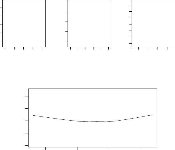
3.5 Residual Plots 105
l
l
l
l
l
l
l
l
l
l
l
l
l
l
l
l
l
l
l
l
l
l
l
l
l
l
l
l
l
l
l
l
l
l
l
l
l
l
l
l
l
l
l
l
l
l
l
l
l
l
l
l
l
l
l
l
l
l
l
l
l
l
l
l
l
l
l
l
l
l
l
l
l
l
l
l
l
l
l
l
l
l
l
l
l
l
l
l
l
l
l
l
l
l
l
l
l
l
l
l
l
−0.10 0.00 0.10
−2
−1
0
1
2
Ideal plot: no pattern
Fitted values μ
^
Std Residuals r
'
l
l
l
l
l
l
l
l
l
l
l
l
l
l
l
l
l
l
l
l
l
l
l
l
l
l
l
l
l
l
l
l
l
l
l
l
l
l
l
l
l
l
l
l
l
l
l
l
l
l
l
l
l
l
l
l
l
l
l
l
l
l
l
l
l
l
l
l
l
l
l
l
l
l
l
l
l
l
l
l
l
l
l
l
l
l
l
l
l
l
l
l
l
l
l
l
l
l
l
l
012345
−2
−1
0
1
2
Non−linearity
Fitted values μ
^
Std Residuals r '
l
l
l
l
l
l
l
l
l
l
l
l
l
l
l
l
l
l
l
l
l
l
l
l
l
l
l
l
l
l
l
l
l
l
l
l
l
l
l
l
l
l
l
l
l
l
l
l
l
l
l
l
l
l
l
l
l
l
l
l
l
l
l
l
l
l
l
l
l
l
l
l
l
l
l
l
l
l
l
l
l
l
l
l
l
l
l
l
l
l
l
l
l
l
l
l
l
l
l
l
1234
−3
−2
−1
0
1
2
3
Non−constant variance
Fitted values μ
^
Std Residuals
r '
Fig. 3.4 Some example plots of the standardized residuals r
plotted against the fitted
values ˆμ. The effects are exaggerated from what is usually seen in practice (Sect. 3.5.1)
l
l
l
l
l
l
l
l
l
l
l
l
l
l
l
l
l
l
l
l
l
l
l
l
l
l
l
l
l
l
l
l
l
l
l
l
l
l
l
l
l
l
l
l
l
l
l
l
l
l
l
l
l
l
l
l
l
l
l
l
l
l
l
l
l
l
l
l
l
l
l
l
l
l
l
l
l
l
l
l
l
l
l
l
l
l
l
l
l
l
l
l
l
l
l
l
l
l
l
l
l
l
l
l
l
l
l
l
l
l
l
l
l
l
l
l
l
l
l
l
l
l
l
l
l
l
l
l
l
l
l
l
l
l
l
l
l
l
l
l
l
l
l
l
l
l
l
l
l
l
l
l
l
l
l
l
l
l
l
l
l
l
l
l
l
l
l
l
l
l
l
l
l
l
l
l
l
l
l
l
l
l
l
l
l
l
l
l
l
l
l
l
l
l
l
l
l
l
l
l
l
l
l
l
l
l
l
l
l
l
l
l
l
l
l
l
l
l
l
l
l
l
l
l
l
l
l
l
l
l
l
l
l
l
l
l
l
l
l
l
l
l
l
l
l
l
l
l
l
l
l
l
l
l
l
l
l
l
l
l
l
l
l
l
l
l
l
l
l
l
l
l
l
l
l
l
l
l
l
l
l
l
l
l
l
l
l
l
l
l
l
l
l
l
l
l
l
l
l
l
l
l
l
l
l
l
l
l
l
l
l
l
l
l
l
l
l
l
l
l
l
l
l
l
l
l
l
l
l
l
l
l
l
l
l
l
l
l
l
l
l
l
l
l
l
l
l
l
l
l
l
l
l
l
l
l
l
l
l
l
l
l
l
l
l
l
l
l
l
l
l
l
ll
l
l
l
l
l
l
l
l
l
l
l
l
l
l
l
l
l
l
l
l
l
l
l
l
l
l
l
l
l
l
l
l
l
l
l
l
l
l
l
l
l
l
l
l
l
l
l
l
l
l
l
l
l
l
l
l
l
l
l
l
l
l
l
l
l
l
l
l
l
l
l
l
l
l
l
l
l
l
l
l
l
l
l
l
l
l
l
l
l
l
l
l
l
l
l
l
l
l
l
l
l
l
l
l
l
l
l
l
l
l
l
l
l
l
l
l
l
l
l
l
l
l
l
l
l
l
l
l
l
l
l
l
l
l
l
l
l
l
l
l
l
l
l
l
l
l
l
l
l
l
l
l
l
l
l
l
l
l
l
l
l
l
l
l
l
l
l
l
l
l
l
l
l
l
l
l
l
l
l
l
l
l
l
l
l
l
l
l
l
l
l
l
l
l
l
l
l
l
l
l
l
l
l
l
l
l
l
l
l
l
l
l
l
l
l
l
l
l
l
l
l
l
l
l
l
l
l
l
l
l
l
l
l
ll
l
l
l
l
l
l
l
l
l
l
l
l
l
l
l
l
l
l
l
l
l
l
l
l
l
l
l
l
l
l
l
l
l
l
l
l
l
l
l
l
l
l
l
l
l
1234
−4
−2
0
2
4
Fitted values
Standardized residuals
Fig. 3.5 Standardized residual plotted against the fitted values for the model LC.lm
fitted to the lung capacity data (Example 3.5)
> # Plot std residuals against the fitted values
> scatter.smooth( rstandard( LC.lm ) ~ fitted( LC.lm ), col="grey",
las=1, ylab="Standardized residuals", xlab="Fitted values")
3.5.4 Q–Q Plots and Normality
The assumption of normality can be checked using a normal quantile–quantile
plot, or normal Q–Q plot, of the residuals. A Q–Q plot, in general, graphs
the quantiles of the data against the quantiles of given distribution; a normal
Q–Q plot graphs the quantiles of the data against the quantiles of a standard
normal distribution. For example, the value below which 30% of the data lie is
plotted against the value below which 30% of a standard normal distribution
lies. If the residuals have a normal distribution, the points will lie on a straight
106 3 Linear Regression Models: Diagnostics and Model-Building
line in the Q–Q plot. For this reason, a straight line is often added to the
Q–Q plot to assist in assessing normality. For small sample sizes, Q–Q plots
may be hard to assess (Problem 3.5).
Non-normality may appear as positive skewness (which is quite common);
negative skewness; as having too many observations in the tails of the dis-
tribution; or as having too few observations in the tails of the distribution
(Fig. 3.6). Q–Q plots are also a convenient way to check for the presence of
large residuals (Sect. 3.6.2). Since standardized residuals r
are more normally
distributed than raw residuals, Q–Q plots are more appropriate and outliers
are easier to identify using standardized residuals.
In r, Q–Q plots of residuals can be produced from a fitted model fit
using qqnorm(), using either resid(fit) or rstandard(fit) as the input.
A reference line for assessing normality of the points is added by following the
qqnorm() command with the corresponding qqline() command, as shown
in the following example.
Example 3.6. Consider the lungcap data again (Example 1.1), and model
LC.lm fitted to the data. The Q–Q plot (Fig. 3.7) suggests that the normality
assumption is suspect:
> # Q-Q probability plot
> qqnorm( rstandard( LC.lm ), las=1, pch=19)
> qqline( rstandard( LC.lm ) ) # Add reference line
The distribution of residuals appears to have heavier tails than the normal
distribution in both directions, because the residuals curve above the line
on the right and below the line on the left. The plot also shows a number
of large residuals, both positive and negative, suggesting the model can be
improved.
3.5.5 Lag Plots and Dependence over Time
Dependence is not always easy to detect, if not already obvious from the data
collection process. When data are collected over time, dependence between
successive response can be detected by plotting each residual against the
previous residual in time, often called the lagged residual. If the responses are
independent, the plots should show no pattern under (Fig. 3.8, left panel).
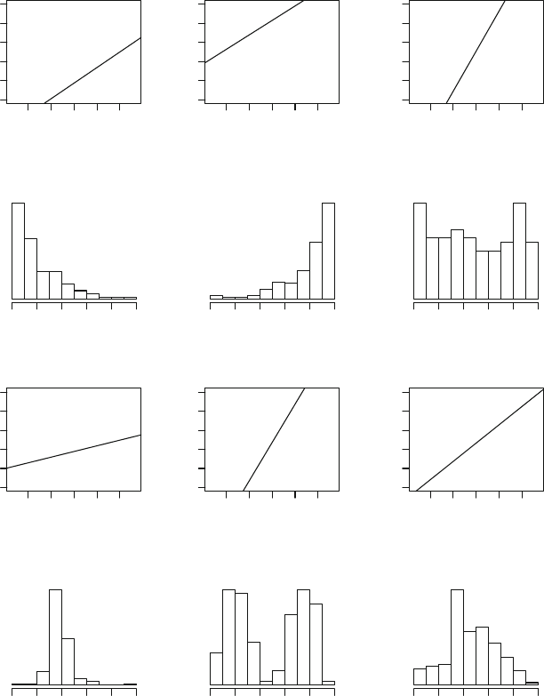
l
l
l
l
l
l
l
l
l
l
l
l
l
l
l
l
l
l
l
l
l
l
l
l
l
l
l
l
l
l
l
l
l
l
l
l
l
l
l
l
l
l
l
l
l
l
l
l
l
l
l
l
l
l
l
l
l
l
l
l
l
l
l
l
l
l
l
l
l
l
l
l
l
l
l
l
l
l
l
l
l
l
l
l
l
l
l
l
l
l
l
l
l
l
l
l
l
l
l
l
l
l
l
l
l
l
l
l
l
l
l
l
l
l
l
l
l
l
l
l
l
l
l
l
l
l
l
l
l
l
l
l
l
l
l
l
l
l
l
l
l
l
l
l
l
l
l
l
l
l
l
−2 −1 0 1 2
0
2
4
6
8
10
Right skewed
Theoretical Quantiles
Sample Quantiles
l
l
l
l
l
l
l
l
l
l
l
l
l
l
l
l
l
l
l
l
l
l
l
l
l
l
l
l
l
l
l
l
l
l
l
l
l
l
l
l
l
l
l
l
l
l
l
l
l
l
l
l
l
l
l
l
l
l
l
l
l
l
l
l
l
l
l
l
l
l
l
l
l
l
l
l
l
l
l
l
l
l
l
l
l
l
l
l
l
l
l
l
l
l
l
l
l
l
l
l
l
l
l
l
l
l
l
l
l
l
l
l
l
l
l
l
l
l
l
l
l
l
l
l
l
l
l
l
l
l
l
l
l
l
l
l
l
l
l
l
l
l
l
l
l
l
l
l
l
l
−2 −1 0 1 2
0
2
4
6
8
10
Left skewed
Theoretical Quantiles
Sample Quantiles
l
l
l
l
l
l
l
l
l
l
l
l
l
l
l
l
l
l
l
l
l
l
l
l
l
l
l
l
l
l
l
l
l
l
l
l
l
l
l
l
l
l
l
l
l
l
l
l
l
l
l
l
l
l
l
l
l
l
l
l
l
l
l
l
l
l
l
l
l
l
l
l
l
l
l
l
l
l
l
l
l
l
l
l
l
l
l
l
l
l
l
l
l
l
l
l
l
l
l
l
l
l
l
l
l
l
l
l
l
l
l
l
l
l
l
l
l
l
l
l
l
l
l
l
l
l
l
l
l
l
l
l
l
l
l
l
l
l
l
l
l
l
l
l
l
l
l
l
l
l
−2 −1 0 1 2
0
2
4
6
8
10
Tails too light
Theoretical Quantiles
Sample Quantiles
Right skewed
Residuals
Frequency
0246810
Left skewed
Residuals
Frequency
0246810
Tails too light
Residuals
Frequency
0246810
l
l
l
l
l
l
l
l
l
l
l
l
l
l
l
l
l
l
l
l
l
l
l
l
l
l
l
l
l
l
l
l
l
l
l
l
l
l
l
l
l
l
l
l
l
l
l
l
l
l
l
l
l
l
l
l
l
l
l
l
l
l
l
l
l
l
l
l
l
l
l
l
l
l
l
l
l
l
l
l
l
l
l
l
l
l
l
l
l
l
l
l
l
l
l
l
l
l
l
l
l
l
l
l
l
l
l
l
l
l
l
l
l
l
l
l
l
l
l
l
l
l
l
l
l
l
l
l
l
l
l
l
l
l
l
l
l
l
l
l
l
l
l
l
l
l
l
l
l
l
−2 −1 0 1 2
0
2
4
6
8
10
Tails too heavy
Theoretical Quantiles
Sample Quantiles
l
l
l
l
l
l
l
l
l
l
l
l
l
l
l
l
l
l
l
l
l
l
l
l
l
l
l
l
l
l
l
l
l
l
l
l
l
l
l
l
l
l
l
l
l
l
l
l
l
l
l
l
l
l
l
l
l
l
l
l
l
l
l
l
l
l
l
l
l
l
l
l
l
l
l
l
l
l
l
l
l
l
l
l
l
l
l
l
l
l
l
l
l
l
l
l
l
l
l
l
l
l
l
l
l
l
l
l
l
l
l
l
l
l
l
l
l
l
l
l
l
l
l
l
l
l
l
l
l
l
l
l
l
l
l
l
l
l
l
l
l
l
l
l
l
l
l
l
l
l
−2 −1 0 1 2
0
2
4
6
8
10
Bimodal distribution
Theoretical Quantiles
Sample Quantiles
l
l
l
l
l
l
l
l
l
l
l
l
l
l
l
l
l
l
l
l
l
l
l
l
l
l
l
l
l
l
l
l
l
l
l
l
l
l
l
l
l
l
l
l
l
l
l
l
l
l
l
l
l
l
l
l
l
l
l
l
l
l
l
l
l
l
l
l
l
l
l
l
l
l
l
l
l
l
l
l
l
l
l
l
l
l
l
l
l
l
l
l
l
l
l
l
l
l
l
l
l
l
l
l
l
l
l
l
l
l
l
l
l
l
l
l
l
l
l
l
l
l
l
l
l
l
l
l
l
l
l
l
l
l
l
l
l
l
l
l
l
l
l
l
l
l
l
l
l
l
−2 −1 0 1 2
0
2
4
6
8
10
True normal distribution
Theoretical Quantiles
Sample Quantiles
Tails too heavy
Residuals
Frequency
0246810
Bimodal distribution
Residuals
Frequency
0246810
True normal distribution
Residuals
Frequency
0246810
Fig. 3.6 Typical Q–Q plots of standardized residuals. In all cases, the sample size is
150. The solid line is added as a reference to aid is assessing linearity of the points
(Sect. 3.5.4)

108 3 Linear Regression Models: Diagnostics and Model-Building
l
l
l
l
l
l
l
l
l
l
l
l
l
l
l
l
l
l
l
l
l
l
l
l
l
l
l
l
l
l
l
l
l
l
l
l
l
l
l
l
l
l
l
l
l
l
l
l
l
l
l
l
l
l
l
l
l
l
l
l
l
l
l
l
l
l
l
l
l
l
l
l
l
l
l
l
l
l
l
l
l
l
l
l
l
l
l
l
l
l
l
l
l
l
l
l
l
l
l
l
l
l
l
l
l
l
l
l
l
l
l
l
l
l
l
l
l
l
l
l
l
l
l
l
l
l
l
l
l
l
l
l
l
l
l
l
l
l
l
l
l
l
l
l
l
l
l
l
l
l
l
l
l
l
l
l
l
l
l
l
l
l
l
l
l
l
l
l
l
l
l
l
l
l
l
l
l
l
l
l
l
l
l
l
l
l
l
l
l
l
l
l
l
l
l
l
l
l
l
l
l
l
l
l
l
l
l
l
l
l
l
l
l
l
l
l
l
l
l
l
l
l
l
l
l
l
l
l
l
l
l
l
l
l
l
l
l
l
l
l
l
l
l
l
l
l
l
l
l
l
l
l
l
l
l
l
l
l
l
l
l
l
l
l
l
l
l
l
l
l
l
l
l
l
l
l
l
l
l
l
l
l
l
l
l
l
l
l
l
l
l
l
l
l
l
l
l
l
l
l
l
l
l
l
l
l
l
l
l
l
l
l
l
l
l
l
l
l
l
l
l
l
l
l
l
l
l
l
l
l
l
l
l
l
l
l
l
l
l
l
l
l
l
l
l
l
l
l
l
l
l
l
l
l
l
l
l
l
l
l
l
l
l
l
l
l
l
l
l
l
l
l
l
ll
l
l
l
l
l
l
l
l
l
l
l
l
l
l
l
l
l
l
l
l
l
l
l
l
l
l
l
l
l
l
l
l
l
l
l
l
l
l
l
l
l
l
l
l
l
l
l
l
l
l
l
l
l
l
l
l
l
l
l
l
l
l
l
l
l
l
l
l
l
l
l
l
l
l
l
l
l
l
l
l
l
l
l
l
l
l
l
l
l
l
l
l
l
l
l
l
l
l
l
l
l
l
l
l
l
l
l
l
l
l
l
l
l
l
l
l
l
l
l
l
l
l
l
l
l
l
l
l
l
l
l
l
l
l
l
l
l
l
l
l
l
l
l
l
l
l
l
l
l
l
l
l
l
l
l
l
l
l
l
l
l
l
l
l
l
l
l
l
l
l
l
l
l
l
l
l
l
l
l
l
l
l
l
l
l
l
l
l
l
l
l
l
l
l
l
l
l
l
l
l
l
l
l
l
l
l
l
l
l
l
l
l
l
l
l
l
l
l
l
l
l
l
l
l
l
l
l
l
l
l
l
l
l
ll
l
l
l
l
l
l
l
l
l
l
l
l
l
l
l
l
l
l
l
l
l
l
l
l
l
l
l
l
l
l
l
l
l
l
l
l
l
l
l
l
l
l
l
l
l
−3 −2 −1 0 1 2 3
−4
−2
0
2
4
Normal Q−Q Plot
Theoretical Quantiles
Sample Quantiles
Fig. 3.7 The Q–Q plot for model LC.lm fitted to the lung capacity data (Example 3.6)
l
l
l
l
l
l
l
l
l
l
l
l
l
l
l
l
l
l
l
l
l
l
l
l
l
l
l
l
l
l
l
l
l
l
l
l
l
l
l
l
l
l
l
l
l
l
l
l
l
l
l
l
l
l
l
l
l
l
l
l
l
l
l
l
l
l
l
l
l
l
l
l
l
l
l
l
l
l
l
l
l
l
l
l
l
l
l
l
l
l
l
l
l
l
l
l
l
l
l
l
−3
−2
−1
0
1
2
3
−3
−2
−1
0
1
2
3
Independent residuals
r
t−1
r
t
l
l
l
l
l
l
l
l
l
l
l
l
l
l
l
l
l
l
l
l
l
l
l
l
l
l
l
l
l
l
l
l
l
l
l
l
l
l
l
l
l
l
l
l
l
l
l
l
l
l
l
l
l
l
l
l
l
l
l
l
l
l
l
l
l
l
l
l
l
l
l
l
l
l
l
l
l
l
l
l
l
l
l
l
l
l
l
l
l
l
l
l
l
l
l
l
l
l
l
−3
−2
−1
0
1
2
3
−3
−2
−1
0
1
2
3
Negatively correlated
residuals
r
t−1
r
t
l
l
l
l
l
l
l
l
l
l
l
l
l
l
l
l
l
l
l
l
l
l
l
l
l
l
l
l
l
l
l
l
l
l
l
l
l
l
l
l
l
l
l
l
l
l
l
l
l
l
l
l
l
l
l
l
l
l
l
l
l
l
l
l
l
l
l
l
l
l
l
l
l
l
l
l
l
l
l
l
l
l
l
l
l
l
l
l
l
l
l
l
l
l
l
l
l
l
l
−3
−2
−1
0
1
2
3
−3
−2
−1
0
1
2
3
Positively correlated
residuals
r
t−1
r
t
Fig. 3.8 Some example plots of the residuals at time t, denoted r
t
, plotted against the
previous residual in time r
t−1
(Sect. 3.5.5)
3.6 Outliers and Influential Observations
3.6.1 Introduction
The previous section presented tools for assessing overall model assumptions.
This section discusses methods for detecting problems with individual obser-
vations. The two issues may be related: an incorrect model specification may
indicate problems with a particular observation. Consequently, the methods
in Sect. 3.5 should be used in conjunction with the methods in this section.

3.6 Outliers and Influential Observations 109
3.6.2 Outliers and Studentized Residuals
Outliers are observations inconsistent with the rest of the data set. Incon-
sistent observations are located by identifying the corresponding residual as
unusually large (positive or negative). This may be done by using Q–Q plots
or other plots already produced for assessing the model assumptions. As a
guideline, potential outliers might be flagged as observations with standard-
ized residual r
greater than, say, 2.5 in absolute value. This is naturally only
a guideline to guide further investigation, as approximately 1.2% of observa-
tions will have absolute standardized residuals exceeding 2.5 just by chance
even when there are no outliers and all the model assumptions are correct.
Standardized residuals are computed using s
2
, which is computed from
the entire data set. An observation with a large raw residual is actually used
to compute s
2
and perhaps inflating its value, in turn making the unusual
observation hard to detect. This suggests omitting Observation i from the cal-
culation of s
2
when computing the residual for Observation i. These residuals
are called Studentized residuals.
To find the Studentized residual r
i
, first fit a linear regression model to
all the data except case i. Then compute the estimate of the variance s
2
(i)
from this model based on the remaining n −1 observations, the subscript (i)
indicating that Observation i has been omitted in computing the estimate.
Then, the Studentized residuals are
r
i
=
√
w
i
(y
i
− ˆμ
i(i)
)
s
(i)
√
1 − h
i
, (3.5)
where ˆμ
i(i)
is the fitted value for Observation i computed from the model
fitted without Observation i. This definition appears to be cumbersome to
compute, since computing r
i
for all n observations apparently requires fitting
n+1 models (the original with all observations, plus a model when each obser-
vation is omitted). However, numerical identities are available for computing
r
i
without the need for repeated linear regressions. Using r, Studentized
residuals are easily found using rstudent().
Example 3.7. For the lungcap data, the residual plot in Fig. 3.2 (p. 102)
shows no outliers (but does shows some large residuals, both positive and
negative), so r
and r
are expected to be similar:
> summary( cbind( Standardized = rstandard(LC.lm),
Studentized = rstudent(LC.lm) ) )
Standardized Studentized
Min. :-3.922299 Min. :-3.966502
1st Qu.:-0.596599 1st Qu.:-0.596304
Median : 0.002062 Median : 0.002061
Mean : 0.000213 Mean : 0.000387
3rd Qu.: 0.559121 3rd Qu.: 0.558826
Max. : 4.885392 Max. : 4.973802

110 3 Linear Regression Models: Diagnostics and Model-Building
Example 3.8. For the model LC.lm fitted to the lungcap data in Example 3.1,
the Studentized residuals can be computed by manually deleting each ob-
servation. For example, deleting Observation 1 and refitting produces the
Studentized residual for Observation 1:
> # Fit the model *without* Observation 1:
> LC.no1 <- lm( FEV ~ Ht + Gender + Smoke,
data=lungcap[-1,]) # The negative index *removes* row 1
> # The fitted value for Observation 1, from the original model:
> mu <- fitted( LC.lm )[1]
> # The estimate of s from the new model, without Obs. 1:
> s <- summary(LC.no1)$sigma
> h <- hatvalues( LC.lm )[1] # Hat value, for Observation 1
> resid.stud <- ( lungcap$FEV[1] - mu ) /(s*sqrt(1-h) )
> resid.stud
1
1.104565
> rstudent(LC.lm)[1] # The easy way
1
1.104565
3.6.3 Influential Observations
Influential observations are observations that substantially change the fitted
model when omitted from the data set. Influential observations necessarily
have moderate to large residuals, but are not necessarily outliers. Similarly,
outliers may or may not be influential.
More specifically, influential observations are those that combine large
residuals with high leverage (Fig. 3.9). That is, influential observations are
outliers with high leverage. A popular measure of influence for observation i
is Cook’s distance:
D =
(r
)
2
p
h
1 − h
. (3.6)
(The subscript i has been omitted here from all quantities for brevity.)
Problem 3.4 develops another interpretation. The values of Cook’s distance
are found in r using cooks.distance().
Approximately, D has an F -distribution with (p
,n− p
) degrees of free-
dom [9], so a conservative approach for identifying influential observations
uses the 50th percentile point of the F -distribution as a guideline [39]. This
guideline is used by r. For most F -distributions, the 50th percentile is near
1, so a useful rule-of-thumb is that observations with D>1 may be flagged
as potentially influential. Other guidelines also exist for identifying high-
influence outliers [10, 12].

3.6 Outliers and Influential Observations 111
Outlier with high influence
x
y
l
l
l
l
l
l
l
l
l
l
ll
Outlier with low influence
x
y
l
l
l
l
l
l
l
l
l
l
ll
No outliers; no high
influence observations
x
y
l
l
l
l
l
l
l
l
l
l
l
Fig. 3.9 Three examples showing the relationship between outliers and influential ob-
servations. The solid circle is the outlier, the solid line is the regression line including
the outlier; the dashed line is the regression line omitting the outlier (Sect. 3.6.3)
Another measure of the influence of Observation i, very similar to Cook’s
distance, is dffits. dffits measures how much the fitted value of Obser-
vation i changes between the model fitted with all the data and the model
fitted when Observation i is omitted:
dffits
i
=
ˆμ
i
− ˆμ
i(i)
s
(i)
= r
i
h
i
1 − h
i
,
where ˆμ
i(i)
is the estimate of μ
i
from the model fitted after omitting Obser-
vation i from the data. dffits
i
is essentially equivalent to the square root of
Cook’s distance. dffits
2
i
differs from Cook’s distance only by a factor of 1/p
and by replacing s
i
with s
(i)
. dffits are computed in r using dffits().
dfbeta is a coefficient-specific version of dffits, which measures how
much the estimates of each individual regression coefficient change between
the model fitted using all observations and the model fitted with Observation i
omitted:
dfbetas
i
=
ˆ
β
j
−
ˆ
β
j(i)
se(
ˆ
β
j(i)
)
,
where
ˆ
β
j(i)
is the estimate of β
j
after omitting Observation i and se(
ˆ
β
j(i)
)is
the standard error of
ˆ
β
j
using s
(i)
to estimate the error standard deviation.
One set of dfbetas is produced for each model coefficient. The dfbetas are
computed in r using dfbetas().
Yet another measure of influence, the covariance ratio (cr), measures the
increase in uncertainty about the regression coefficients when Observation i
is omitted. Mathematically, cr is the ratio by which the volume of the con-
fidence ellipsoid for the coefficient vector increases when Observation i is

112 3 Linear Regression Models: Diagnostics and Model-Building
omitted. More simply, the square root of cr can be interpreted as the av-
erage factor by which the confidence intervals for the regression coefficients
become wider when Observation i is omitted. A convenient computational
formula for cr is:
cr =
1
1 − h
n − p
n − p
+(r
)
2
p
,
where r
is the Studentized residual (3.5). In r, the function covratio()
computes cr.
The r function influence.measures() produces a table of the influence
measures dfbetas, dffits, cr and D, plus the leverages h. Observations
identified as influential with respect to any of these statistics (or having high
leverage in the case of h) are flagged with a * according to the following
criteria:
• dfbetas: Observation i is declared influential when |dfbetas
i
| > 1.
• dffits: Observation i is declared influential when
|dffits
i
| > 3/
p
/(n − p
).
• Covariance ratio cr: Observation i is declared influential when cr
i
>
3p
/(n − p
).
• Cook’s distance D: Observation i is declared influential when D exceeds
the 50th percentile of the F distribution with (p
,n−p
) degrees of free-
dom.
• Leverages h: Observations are declared high leverage if h>3p
/n.
Different observations may be declared as influential by the different criteria.
The covariance ratio has a tendency to declare more observations as influen-
tial than the other criteria.
Example 3.9. Consider the lung capacity data again (Example 1.1; data set:
lungcap), and model LC.lm (Example 3.1,p.97). The observations with the
smallest and largest values of Cook’s distance are:
> cd.max <- which.max( cooks.distance(LC.lm)) # Largest D
> cd.min <- which.min( cooks.distance(LC.lm)) # Smallest D
> c(Min.Cook = cd.min, Max.Cook = cd.max)
Min.Cook.69 Max.Cook.613
69 613
The values of dffits, cv and Cook’s distance for these observations can be
found as follows:
> out <- cbind( DFFITS=dffits(LC.lm),
Cooks.distance=cooks.distance(LC.lm),
Cov.ratio=covratio(LC.lm))
3.6 Outliers and Influential Observations 113
These statistics for the observations cd.max and cd.min are:
> round( out[c(cd.min, cd.max),], 5) # Show the values for these obs only
DFFITS Cooks.distance Cov.ratio
69 0.00006 0.00000 1.01190
613 -0.39647 0.03881 0.96737
From these three measures, Observation 613 is more influential than Observa-
tion 69 according to dffits and Cook’s distance (but not cv). Now examine
influence of Observation 613 and 69 on each of the regression parameters:
> dfbetas(LC.lm)[cd.min,] # Show DBETAS for cd.min
(Intercept) Ht GenderM SmokeSmoker
4.590976e-05 -3.974922e-05 -2.646158e-05 -1.041249e-06
> dfbetas(LC.lm)[cd.max,] # Show DBETAS for cd.max
(Intercept) Ht GenderM SmokeSmoker
0.05430730 -0.06394615 0.10630441 -0.31682958
Omitting Observation 69 (cd.min) makes almost no difference to the re-
gression coefficients. Observation 613 is clearly more influential than Obser-
vation 69, as expected. The r function influence.measures() is used to
identify potentially influential observations according to r’s criteria:
> LC.im <- influence.measures( LC.lm ); names(LC.im)
[1] "infmat" "is.inf" "call"
The object LC.im contains the influence statistics (as LC.im$infmat), and
whether or not they are influential according to r’s criteria (LC.im$is.inf):
> head( round(LC.im$infmat, 3) ) # Show for first few observations only
dfb.1_ dfb.Ht dfb.GndM dfb.SmkS dffit cov.r cook.d hat
1 0.117 -0.109 -0.024 0.015 0.127 1.012 0.004 0.013
2 -0.005 0.005 0.001 -0.001 -0.006 1.017 0.000 0.010
3 0.051 -0.047 -0.014 0.005 0.058 1.015 0.001 0.010
4 0.113 -0.104 -0.031 0.012 0.127 1.007 0.004 0.010
5 0.116 -0.106 -0.036 0.010 0.133 1.004 0.004 0.009
6 0.084 -0.077 -0.026 0.007 0.097 1.009 0.002 0.009
> head( LC.im$is.inf )
dfb.1_ dfb.Ht dfb.GndM dfb.SmkS dffit cov.r cook.d hat
1 FALSE FALSE FALSE FALSE FALSE FALSE FALSE FALSE
2 FALSE FALSE FALSE FALSE FALSE FALSE FALSE FALSE
3 FALSE FALSE FALSE FALSE FALSE FALSE FALSE FALSE
4 FALSE FALSE FALSE FALSE FALSE FALSE FALSE FALSE
5 FALSE FALSE FALSE FALSE FALSE FALSE FALSE FALSE
6 FALSE FALSE FALSE FALSE FALSE FALSE FALSE FALSE
To determine how many entries in the columns of LC.im$is.inf are TRUE,
sum over the columns (this works because r treats FALSE as 0 and TRUE as 1):
> colSums( LC.im$is.inf )
dfb.1_ dfb.Ht dfb.GndM dfb.SmkS dffit cov.r cook.d hat
0000185607

114 3 Linear Regression Models: Diagnostics and Model-Building
Seven observations have high leverage, as identified by the column labelled
hat, 56 observations are identified by the covariance ratio as influential, but
Cook’s distance does not identify any observation as influential.
We can also determine how many criteria declare observations as influential
by summing the relevant columns of LC.im$is.inf over the rows:
> table( rowSums( LC.im$is.inf[, -8] ) ) # Omitting leverages (col 8)
012
590 54 10
This shows that most observations are not declared influential on any of the
criteria, and 54 observations declared as influential on just one criterion.
For Observations 69 and 613 explicitly:
> LC.im$is.inf[c(cd.min, cd.max), ]
dfb.1_ dfb.Ht dfb.GndM dfb.SmkS dffit cov.r cook.d hat
69 FALSE FALSE FALSE FALSE FALSE FALSE FALSE FALSE
613 FALSE FALSE FALSE FALSE TRUE TRUE FALSE FALSE
Observation 613 is significantly influential based on dffits and cv.
A plot of these influence diagnostics is often useful (Fig. 3.10), using type=
"h" to draw histogram-like (or high-density) plots:
> # Cooks' Distance
> plot( cooks.distance( LC.lm ), type="h", main="Cook's distance",
ylab="D", xlab="Observation number", las=1 )
> # DFFITS
> plot( dffits( LC.lm ), type="h", main="DFFITS",
ylab="DFFITS", xlab="Observation number", las=1 )
0 200 500
0.00
0.01
0.02
0.03
0.04
Cook's distance
Observation number
D
0 200 500
−0.4
−0.2
0.0
0.2
0.4
DFFITS
Observation number
DFFITS
0 200 500
−0.10
−0.05
0.00
0.05
0.10
0.15
0.20
DFBETAS for beta2
Observation number
DFBETAS
Fig. 3.10 Influence diagnostics for model LC.lm fitted to the lung capacity data. Left
panel: Cook’s distance D
i
; centre panel: dffits; right panel: dfbetas for β
2
(Exam-
ple 3.9)
3.8 Remedies: Fixing Identified Problems 115
> # DFBETAS for beta_2 only (that is, column 3)
> dfbi <- 2
> plot( dfbetas( LC.lm )[, dfbi + 1], type="h", main="DFBETAS for beta2",
ylab="DFBETAS", xlab="Observation number", las=1 )
3.7 Terminology for Residuals
The terminology used for residuals is confusingly inconsistent. Generally in
statistics, dividing some quantity by an estimate of its standard deviation
is called standardizing. More specifically, dividing a quantity which follows a
normal distribution by the sample standard deviation to produce a quantity
which follows a t-distribution is called Studentizing, following the approach
used by Student [37] when introducing the t-distribution.
Under these commonly-used definitions, both r
and r
are standardized
and Studentized residuals, and various authors use the terms for describing
both residuals. Following r and Belsley et al. [3], we call r
the Studen-
tized residual (Sect. 3.6.2; rstudent() in r) because it follows a Student’s
t-distribution exactly, whereas r
will simply be called the standardized resid-
ual (Sect. 3.3; rstandard() in r).
An alternative convention [39] is to call r
the internally Studentized resid-
ual and r
the externally Studentized residual. These labels are perhaps more
specific and descriptive of the differences between the two types of residuals,
but have not become widely used in the literature.
3.8 Remedies: Fixing Identified Problems
The past few sections have described a variety of diagnostics for identifying
different types of weaknesses in the fitted model. The next few sections will
consider some standard strategies for modifying the fitted model in order to
remedy or ameliorate specific problems.
One commonly-occurring problem is that the response is recorded on a
measurement scale for which the variance increases or decreases with the
mean. If this is the case, the variance can often be stabilized by transforming
the response to a different scale (Sect. 3.9).
Sometimes a nonlinear relationship between y and x canbefixedbya
simple transformation of x (Sect. 3.10). More generally, a complex relation-
ship between a covariate and the response signals the need to build further
terms into the model to capture this relationship (Sections 3.11 and 3.12).
Usually the measurement scale of y should be settled before transforming
116 3 Linear Regression Models: Diagnostics and Model-Building
the covariates, because any transformation of y will obviously impact on the
shape of its relationships with the covariates.
Often the above steps will solve structural problems and hence also tend
to reduce the number of apparent outliers or dangerously influential observa-
tions. If some remain, however, decisions must be made to remove the out-
liers or to accommodate them into a modified model. Section 3.13 discusses
these issues.
One possible problem that will not be discussed in detail later is that
of correlated residuals. Dependence between responses can arise from com-
mon causes shared between observations, or from a carryover effect from
one observation to another, or from other causes. When the responses fail
to be independent, there are a variety of more complex models that can
be developed to accommodate this dependence, including generalized least
squares [8], mixed models [40] or spatial models [5]. All of these possibilities
however would take us outside the scope of this book.
3.9 Transforming the Response
3.9.1 Symmetry, Constraints and the Ladder of
Powers
The idea of a transformation is to convert the response variable to a different
measurement scale. For example, consider the acidity of swimming pool wa-
ter. From a chemical point of view, acidity is measured by the concentration
of hydrogen ions. However acidity is more commonly expressed in terms of
pH-level. If y is hydrogen ion concentration, then the pH level is defined by
pH= −log
10
y. This serves as an alternative and, for many purposes, more
useful scale on which to measure the same quantity. In mathematical terms,
a new response variable y
∗
= h(y) is computed from y, where h() is some
invertible function, and then a linear regression model is built for y
∗
instead
of y. In the case of the pH-level, h(y)=−log
10
y. After transforming the
response, the basic linear regression model structure remains the same, the
new variable y
∗
simply replacing y. The model becomes
y
∗
i
∼ N(μ
i
,σ
2
)
μ
i
= β
0
+
p
j=1
β
j
x
ij
.
(3.7)
Note that now μ
i
=E[y
∗
i
] rather than E[y
i
]. After transforming the response,
one will typically refit the model and produce new residual plots to recheck
assumptions for the new model. This may be done iteratively until a satis-
factory transformation is found.
There are three main reasons why one might choose to transform the re-
sponse variable. First, transforming the measurement scale so that it covers
3.9 Transforming the Response 117
the whole real line can avoid difficulties with constraints on the linear regres-
sion coefficients. In the lung capacity study, for example, ideally we would
like to ensure that our model will never predict a negative value for fev.The
difficulty with predicting negative values for fev can be avoiding by building
a linear regression model for y
∗
= log(fev) instead of for fev itself, because
any predicted value for the logarithm of fev, whether negative or positive,
translates into a positive value for fev itself.
When y is a count for which zero is a possible value, the starred log-
transformations y
∗
= log (y +0.5) or y
∗
= log (y + 1) have been used to
avoid taking the logarithm of zero. When y is a count out of a possible total
n, then the empirical logistic transformation y
∗
= log{(y +0.5)/(n+0.5)} has
sometimes been used. In both cases the motivation is the same: to convert
the response to a scale for which the linear predictor is unconstrained. These
transformations can be successful if the counts are not too small or too near
the boundary values.
A second possible reason for transforming the response is to cause its
distribution to be more nearly normally distributed. Typically this means
trying to make the distribution of y-values more symmetric. For example,
consider the acidity of swimming pool water again. The concentration of
hydrogen ions is a strictly positive quantity, usually very close to zero but
varying by orders of magnitude from one circumstance to another. Hence
hydrogen concentration is likely have a highly right-skewed distribution. By
contrast, the pH-levels are usually more symmetrically distributed. In other
words, the pH-level is likely to be more nearly normally distributed than
is the hydrogen ion concentration itself. Right skew distributions arise most
commonly when the response measures a physical quantity that can only take
positive values. In such a case, a log-transformation, y
∗
= log y, or a power
transformation, y
∗
= y
λ
with λ<1, will reduce the right skewness. Common
values for λ make up what is sometimes called a ladder of powers (Table 3.1).
The smaller λ is chosen, the stronger the transformation. A too small value
for λ will reverse a right skew distribution to one that is left skew. The usual
procedure is to start with a transformation with λ near one, then decrease λ
until symmetry of the residuals from the regression is roughly achieved.
If y is left skewed, then a power transformation y
∗
= y
λ
with λ>1 might
be used (Table 3.1). Such situations are less common however.
3.9.2 Variance-Stabilizing Transformations
There is a third and even more fundamental motivation for transforming
the response variable, which is to try to achieve close to constant variance
across all observations. Again we focus on the commonly-occurring situation
in which y measures some physical quantity that can only take on positive
values. For such a variable, it is almost inevitable that the variance of y
will be smaller when μ is close to zero than when μ is large, because of

118 3 Linear Regression Models: Diagnostics and Model-Building
Tabl e 3 .1 The ‘ladder of powers’. Variance increasing with mean is more common than
variance decreasing with the mean, hence the transformations on the right-hand side
are more commonly used. Note that λ = 1 produces no transformation of the response
(Sect. 3.9)
Transformation: ← ... y
3
y
2
y
√
y log y 1/
√
y 1/y 1/y
2
···→
Box–Cox λ: ← ... 32 11/20−1/2 −1 −2 ···→
Primary use: • When variance • When variance increases with
decreases with increasing mean
increasing mean
Other uses: • When y left-skewed • When y right-skewed
the requirement that the range of y is restricted to positive values. This
phenomenon will become readily apparent in practical terms when the values
of y vary by orders of magnitude in a single data set. In these cases, we say
that y shows a positive mean–variance relationship.
In the scientific literature, the uncertainty of physical measurements of
positive quantities are often expressed in terms of the coefficient of variation
(standard deviation divided by the mean) instead of in terms of variance or
standard deviation. This is because the coefficient of variation often tends to
be more nearly constant across cases than is the standard deviation, so it is
more useful to express variability in relative terms rather than in absolute
terms. Mathematically, this means that the standard deviation σ of y is
proportional to the mean μ or, equivalently, the variance is proportional
to the mean squared, var[y]=φμ
2
for some φ. In such cases, y is said to
have a quadratic mean–variance relationship. The strongest motivation for
transforming the response is usually to try to remove the mean–variance
relationship.
If y takes positive values, then the ladder of powers may be used to remove
or mitigate a mean–variance relationship (Table 3.1). A power transformation
with λ<1 will reduce or remove an increasing mean–variance relationship,
while λ>1 will reduce or remove a decreasing mean–variance relationship.
More generally, we consider the class of variance-stabilizing transforma-
tions. Suppose that y has a mean–variance relationship defined by the func-
tion V (μ), with var[y]=φV (μ). Then, consider a transformation y
∗
= h(y).
A first-order Taylor series expansion of h(y)aboutμ gives y
∗
= h(y) ≈
h(μ)+h
(μ)(y −μ), from which it can be inferred that
var[y
∗
]=var[h(y)] ≈ h
(μ)
2
var[y].
Hence the transformation y
∗
= h(y) will approximately stabilize the variance
if h
(μ) is proportional to var[y]
−1/2
= V (μ)
−1/2
. When V (μ)=μ
2
(standard
deviation proportional to the mean), the variance-stabilizing transformation
is the logarithm, because then h
(μ)=1/μ. When V (μ)=μ, the variance-
stabilizing transformation is the square root, because h
(μ)=1/μ
1/2
.

3.9 Transforming the Response 119
The most common variance-stabilizing transformations appear on a ladder
of powers (Table 3.1). To use this ladder, note that the milder transformations
are closer to λ = 1 (no transformation). It is usual to start with mild transfor-
mations and progressively try more severe transformations as necessary. For
example, if a logarithmic transformation still produces increasing variance as
the mean increases, try the next transformation on the ladder: 1/
√
y.The
most commonly-used transformation is the logarithmic transformation.
When y is a proportion or percentage (taking values from zero to one, or
zero to 100%), the mean–variance relationship is likely to be unimodal. In
such cases, the possible values for y have two boundaries, one at zero and
the other at one, and the variance of y is likely to decrease as the mean ap-
proaches either boundary. Proportions often show a quadratic mean–variance
relationship of the form V (μ) ∝ μ(1 − μ), with 0 <μ<1. In such cases, the
variance-stabilizing transformation is the arc-sin–square root transformation
y
∗
=sin
−1
√
y.
Transformations with λ ≤ 0 can only be applied to positive values of y.If
negative values are present, then power transformations should not be used.
If y is positive except for a few exact zeros, one has the choice between using a
positive value of λ, for example a small positive value such as λ =1/4 instead
of a log-transformation, or else offsetting y to be positive before transforming.
For example, a response variable such as rainfall is positive and continuous
on days when rain has occurred, but is zero otherwise. In such cases, the
starred logarithmic transformation, y
∗
= log(y +c) where c is a small positive
constant, has sometimes been used. Such transformations should be used with
caution, as they are sensitive to the choice of offset c. Choosing c too small
can easily introduce outliers into the data.
Example 3.10. For the lungcap data, we have established that the model LC.
lm is inadequate (Example 3.3). For example, a plot of r
against ˆμ
i
(Fig. 3.5)
shows non-constant variance. Various transformations of the response can be
used to determine which, if any, transformation of the response is appropriate
(Fig. 3.11). Since the variance increases with increasing mean, try the first
transformation suggested on the ladder of powers (Table 3.1,p.118), the
square root transformation:
> LC.sqrt <- update( LC.lm, sqrt(FEV) ~ .)
> scatter.smooth( rstandard(LC.sqrt)~fitted(LC.sqrt), las=1, col="grey",
ylab="Standardized residuals", xlab="Fitted values",
main="Square-root transformation")
This transformation (Fig. 3.11, top right panel) produces slightly increasing
variance. Try the next transformation on the ladder, the commonly-used
logarithmic transformation:
> LC.log <- update( LC.lm, log(FEV) ~ .)
> scatter.smooth( rstandard(LC.log)~fitted(LC.log), las=1, col="grey",
ylab="Standardized residuals", xlab="Fitted values",
main="Log transformation")
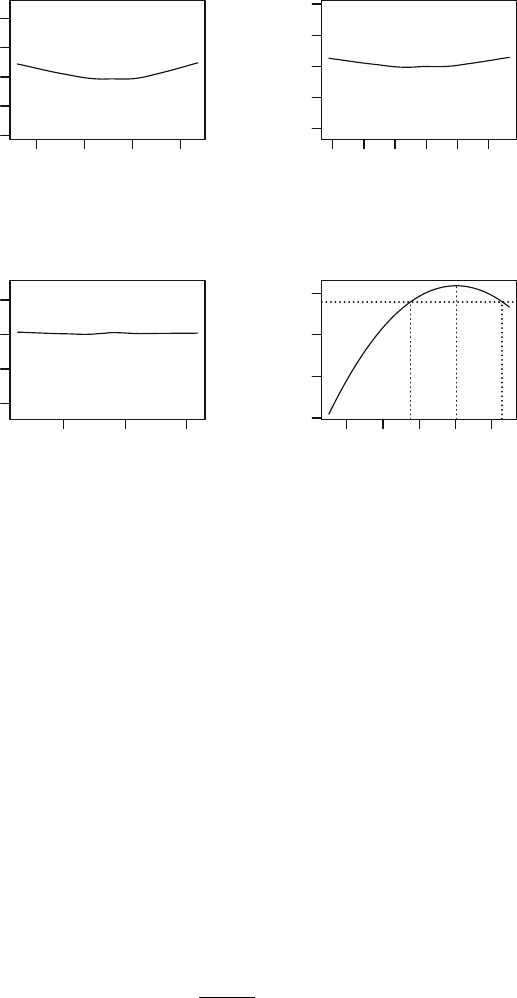
120 3 Linear Regression Models: Diagnostics and Model-Building
l
l
l
l
l
l
l
l
l
l
l
l
l
l
l
l
l
l
l
l
l
l
l
l
l
l
l
l
l
l
l
l
l
l
l
l
l
l
l
l
l
l
l
l
l
l
l
l
l
l
l
l
l
l
l
l
l
l
l
l
l
l
l
l
l
l
l
l
l
l
l
l
l
l
l
l
l
l
l
l
l
l
l
l
l
l
l
l
l
l
l
l
l
l
l
l
l
l
l
l
l
l
l
l
l
l
l
l
l
l
l
l
l
l
l
l
l
l
l
l
l
l
l
l
l
l
l
l
l
l
l
l
l
l
l
l
l
l
l
l
l
l
l
l
l
l
l
l
l
l
l
l
l
l
l
l
l
l
l
l
l
l
l
l
l
l
l
l
l
l
l
l
l
l
l
l
l
l
l
l
l
l
l
l
l
l
l
l
l
l
l
l
l
l
l
l
l
l
l
l
l
l
l
l
l
l
l
l
l
l
l
l
l
l
l
l
l
l
l
l
l
l
l
l
l
l
l
l
l
l
l
l
l
l
l
l
l
l
l
l
l
l
l
l
l
l
l
l
l
l
l
l
l
l
l
l
l
l
l
l
l
l
l
l
l
l
l
l
l
l
l
l
l
l
l
l
l
l
l
l
l
l
l
l
l
l
l
l
l
l
l
l
l
l
l
l
l
l
l
l
l
l
l
l
l
l
l
l
l
l
l
l
l
l
l
l
l
l
l
l
l
l
l
l
l
l
l
l
l
l
l
l
l
l
l
l
l
l
l
l
l
l
l
l
l
l
l
l
l
l
l
l
l
l
l
l
l
l
l
l
l
l
l
l
l
l
l
l
l
l
l
l
ll
l
l
l
l
l
l
l
l
l
l
l
l
l
l
l
l
l
l
l
l
l
l
l
l
l
l
l
l
l
l
l
l
l
l
l
l
l
l
l
l
l
l
l
l
l
l
l
l
l
l
l
l
l
l
l
l
l
l
l
l
l
l
l
l
l
l
l
l
l
l
l
l
l
l
l
l
l
l
l
l
l
l
l
l
l
l
l
l
l
l
l
l
l
l
l
l
l
l
l
l
l
l
l
l
l
l
l
l
l
l
l
l
l
l
l
l
l
l
l
l
l
l
l
l
l
l
l
l
l
l
l
l
l
l
l
l
l
l
l
l
l
l
l
l
l
l
l
l
l
l
l
l
l
l
l
l
l
l
l
l
l
l
l
l
l
l
l
l
l
l
l
l
l
l
l
l
l
l
l
l
l
l
l
l
l
l
l
l
l
l
l
l
l
l
l
l
l
l
l
l
l
l
l
l
l
l
l
l
l
l
l
l
l
l
l
l
l
l
l
l
l
l
l
l
l
l
l
l
l
l
l
l
l
ll
l
l
l
l
l
l
l
l
l
l
l
l
l
l
l
l
l
l
l
l
l
l
l
l
l
l
l
l
l
l
l
l
l
l
l
l
l
l
l
l
l
l
l
l
l
1234
−4
−2
0
2
4
No transformation
Fitted values
Standardized residuals
l
l
l
l
l
l
l
l
l
l
l
l
l
l
l
l
l
l
l
l
l
l
l
l
l
l
l
l
l
l
l
l
l
l
l
l
l
l
l
l
l
l
l
l
l
l
l
l
l
l
l
l
l
l
l
l
l
l
l
l
l
l
l
l
l
l
l
l
l
l
l
l
l
l
l
l
l
l
l
l
l
l
l
l
l
l
l
l
l
l
l
l
l
l
l
l
l
l
l
l
l
l
l
l
l
l
l
l
l
l
l
l
l
l
l
l
l
l
l
l
l
l
l
l
l
l
l
l
l
l
l
l
l
l
l
l
l
l
l
l
l
l
l
l
l
l
l
l
l
l
l
l
l
l
l
l
l
l
l
l
l
l
l
l
l
l
l
l
l
l
l
l
l
l
l
l
l
l
l
l
l
l
l
l
l
l
l
l
l
l
l
l
l
l
l
l
l
l
l
l
l
l
l
l
l
l
l
l
l
l
l
l
l
l
l
l
l
l
l
l
l
l
l
l
l
l
l
l
l
l
l
l
l
l
l
l
l
l
l
l
l
l
l
l
l
l
l
l
l
l
l
l
l
l
l
l
l
l
l
l
l
l
l
l
l
l
l
l
l
l
l
l
l
l
l
l
l
l
l
l
l
l
l
l
l
l
l
l
l
l
l
l
l
l
l
l
l
l
l
l
l
l
l
l
l
l
l
l
l
l
l
l
l
l
l
l
l
l
l
l
l
l
l
l
l
l
l
l
l
l
l
l
l
l
l
l
l
l
l
l
l
l
l
l
l
l
l
l
l
l
l
l
l
l
l
l
l
l
l
l
l
l
l
l
l
l
l
l
l
l
l
l
ll
l
l
l
l
l
l
l
l
l
l
l
l
l
l
l
l
l
l
l
l
l
l
l
l
l
l
l
l
l
l
l
l
l
l
l
l
l
l
l
l
l
l
l
l
l
l
l
l
l
l
l
l
l
l
l
l
l
l
l
l
l
l
l
l
l
l
l
l
l
l
l
l
l
l
l
l
l
l
l
l
l
l
l
l
l
l
l
l
l
l
l
l
l
l
l
l
l
l
l
l
l
l
l
l
l
l
l
l
l
l
l
l
l
l
l
l
l
l
l
l
l
l
l
l
l
l
l
l
l
l
l
l
l
l
l
l
l
l
l
l
l
l
l
l
l
l
l
l
l
l
l
l
l
l
l
l
l
l
l
l
l
l
l
l
l
l
l
l
l
l
l
l
l
l
l
l
l
l
l
l
l
l
l
l
l
l
l
l
l
l
l
l
l
l
l
l
l
l
l
l
l
l
l
l
l
l
l
l
l
l
l
l
l
l
l
l
l
l
l
l
l
l
l
l
l
l
l
l
l
l
l
l
l
ll
l
l
l
l
l
l
l
l
l
l
l
l
l
l
l
l
l
l
l
l
l
l
l
l
l
l
l
l
l
l
l
l
l
l
l
l
l
l
l
l
l
l
l
l
l
1.0 1.4 1.8
−4
−2
0
2
4
Square−root transformation
Fitted values
Standardized residuals
l
l
l
l
l
l
l
l
l
l
l
l
l
l
l
l
l
l
l
l
l
l
l
l
l
l
l
l
l
l
l
l
l
l
l
l
l
l
l
l
l
l
l
l
l
l
l
l
l
l
l
l
l
l
l
l
l
l
l
l
l
l
l
l
l
l
l
l
l
l
l
l
l
l
l
l
l
l
l
l
l
l
l
l
l
l
l
l
l
l
l
l
l
l
l
l
l
l
l
l
l
l
l
l
l
l
l
l
l
l
l
l
l
l
l
l
l
l
l
l
l
l
l
l
l
l
l
l
l
l
l
l
l
l
l
l
l
l
l
l
l
l
l
l
l
l
l
l
l
l
l
l
l
l
l
l
l
l
l
l
l
l
l
l
l
l
l
l
l
l
l
l
l
l
l
l
l
l
l
l
l
l
l
l
l
l
l
l
l
l
l
l
l
l
l
l
l
l
l
l
l
l
l
l
l
l
l
l
l
l
l
l
l
l
l
l
l
l
l
l
l
l
l
l
l
l
l
l
l
l
l
l
l
l
l
l
l
l
l
l
l
l
l
l
l
l
l
l
l
l
l
l
l
l
l
l
l
l
l
l
l
l
l
l
l
l
l
l
l
l
l
l
l
l
l
l
l
l
l
l
l
l
l
l
l
l
l
l
l
l
l
l
l
l
l
l
l
l
l
l
l
l
l
l
l
l
l
l
l
l
l
l
l
l
l
l
l
l
l
l
l
l
l
l
l
l
l
l
l
l
l
l
l
l
l
l
l
l
l
l
l
l
l
l
l
l
l
l
l
l
l
l
l
l
l
l
l
l
l
l
l
l
l
l
l
l
l
l
l
l
l
l
ll
l
l
l
l
l
l
l
l
l
l
l
l
l
l
l
l
l
l
l
l
l
l
l
l
l
l
l
l
l
l
l
l
l
l
l
l
l
l
l
l
l
l
l
l
l
l
l
l
l
l
l
l
l
l
l
l
l
l
l
l
l
l
l
l
l
l
l
l
l
l
l
l
l
l
l
l
l
l
l
l
l
l
l
l
l
l
l
l
l
l
l
l
l
l
l
l
l
l
l
l
l
l
l
l
l
l
l
l
l
l
l
l
l
l
l
l
l
l
l
l
l
l
l
l
l
l
l
l
l
l
l
l
l
l
l
l
l
l
l
l
l
l
l
l
l
l
l
l
l
l
l
l
l
l
l
l
l
l
l
l
l
l
l
l
l
l
l
l
l
l
l
l
l
l
l
l
l
l
l
l
l
l
l
l
l
l
l
l
l
l
l
l
l
l
l
l
l
l
l
l
l
l
l
l
l
l
l
l
l
l
l
l
l
l
l
l
l
l
l
l
l
l
l
l
l
l
l
l
l
l
l
l
l
ll
l
l
l
l
l
l
l
l
l
l
l
l
l
l
l
l
l
l
l
l
l
l
l
l
l
l
l
l
l
l
l
l
l
l
l
l
l
l
l
l
l
l
l
l
l
0.5 1.0 1.5
−4
−2
0
2
Log transformation
Fitted values
Standardized residuals
−0.2 0.0 0.1 0.2
−895
−885
λ
log−Likelihood
95%
Fig. 3.11 Transformations of the fev in the data frame lungcap. The original data
(top left panel); using a square root transformation (top right panel); using a logarithmic
transformation (bottom left panel); a plot to find the Box–Cox transformation (bottom
right panel) (Examples 3.10 and 3.11)
This plot show approximately constant variance and no trend. The logarith-
mic transformation appears suitable, and also allows easier interpretations
than using the square root transformation. A logarithmic transformation of
the response is required to produce almost constant variance, as used in
Chap 2.
3.9.3 Box–Cox Transformations
Notice that the transformations in Table 3.1 have the form of y raised to some
power, except for the logarithmic transformation. The logarithmic transfor-
mation also fits the general power-transformation form if we define
y
∗
=
⎧
⎨
⎩
y
λ
− 1
λ
for λ =0
log y for λ =0.
(3.8)
3.10 Simple Transformations of Covariates 121
This family of transformations is called the Box–Cox transformation [7]. The
form of the Box–Cox transformation (3.8) is continuous in λ when natural
logarithms are used, since (y
λ
−1)/λ → log y as λ → 0. The Box–Cox trans-
formation (3.8) has the same impact as the transformation y
∗
= y
λ
, but the
results differ numerically. For example, λ = 1 transforms the responses y to
(y−1), which has no impact on the model structure, but the numerical values
of the response change.
Computationally, various values of λ are chosen, and the transformation
producing the response y
∗
with approximately constant variance is then cho-
sen. This approach can be implemented in r directly, or by using the function
boxcox() (in the package MASS). The boxcox() function uses the maximum
likelihood criterion, discussed in the next chapter of this book. It finds the
optimal λ to achieve linearity, normality and constant variance simultane-
ously.
Example 3.11. Continuing using the lungcap data from the previous exam-
ple, we use the boxcox() function to estimate the optimal Box–Cox trans-
formation. In the plot produced, higher log-likelihood values are preferable.
The maximum of the Box–Cox plot is achieved when λ is just above zero,
confirming that a logarithmic transformation is close to optimal for achieving
linearity, normality and constant variance (Fig. 3.11, bottom right panel):
> library(MASS) # The function boxcox() is in the MASS package
> boxcox( FEV ~ Ht + Gender + Smoke,
lambda=seq(-0.25, 0.25, length=11), data=lungcap)
3.10 Simple Transformations of Covariates
Sometimes, to achieve linearity or to reduce the influence of influential ob-
servations, transformations of the covariates are required (Fig. 3.12). Using
transformed covariates still produces a model linear in the parameters. Trans-
formations may apply to any or all of the covariates. (Transforming factors
makes no sense.)
Example 3.12. The wind velocity and corresponding direct current (dc) out-
put from windmills (Table 3.2; data set: windmill) was recorded [18, 19].
A plot of the data (Fig. 3.13, left panels) shows non-linearity, but little ev-
idence of non-constant variance (so a transformation of the response is not
recommended):
> data(windmill); names(windmill)
[1] "Wind" "DC"

122 3 Linear Regression Models: Diagnostics and Model-Building
Fig. 3.12 Transformations of covariates to achieve linearity (Sect. 3.10)
Tabl e 3 .2 The dc output from windmills at various wind velocities (in miles/h)
(Example 3.2)
Wind velocity dc output Wind velocity dc output Wind velocity dc output
2.45 0.123 4.60 1.562 7.85 2.179
2.70 0.500 5.00 1.582 8.15 2.166
2.90 0.653 5.45 1.501 8.80 2.112
3.05 0.558 5.80 1.737 9.10 2.303
3.40 1.057 6.00 1.822 9.55 2.294
3.60 1.137 6.20 1.866 9.70 2.386
3.95 1.144 6.35 1.930 10.00 2.236
4.10 1.194 7.00 1.800 10.20 2.310
7.40 2.088
> scatter.smooth( windmill$DC ~ windmill$Wind, main="No transforms",
xlab="Wind speed", ylab="DC output", las=1)
> wm.m1 <- lm( DC ~ Wind, data=windmill )
> scatter.smooth( rstandard(wm.m1) ~ fitted(wm.m1), main="No transforms",
xlab="Standardized residulas", ylab="Fitted values", las=1)
To alleviate the non-linearity, we try some transformations of the wind-
speed. Based on Fig. 3.12, we initially try a logarithmic transformation of
Wind, the most common transformation (Fig. 3.13, centre panels):
> scatter.smooth( windmill$DC ~ log(windmill$Wind), main="Log(Wind)",
xlab="log(Wind speed)", ylab="DC output", las=1)
> wm.m2 <- lm( DC ~ log(Wind), data=windmill )
> scatter.smooth( rstandard(wm.m2) ~ fitted(wm.m2), main="Log(Wind)",
ylab="Standardized residuals", xlab="Fitted values", las=1)

3.10 Simple Transformations of Covariates 123
l
l
l
l
l
l
l
l
l
l
l
l
l
l
l
l
l
l
l
l
l
l
l
l
l
46810
0.5
1.0
1.5
2.0
No transforms
Wind speed
DC output
l
l
l
l
l
l
l
l
l
l
l
l
l
l
l
l
l
l
l
l
l
l
l
l
l
1.0 1.5 2.0 2.5
−2
−1
0
1
No transforms
Standardized residulas
Fitted values
l
l
l
l
l
l
l
l
l
l
l
l
l
l
l
l
l
l
l
l
l
l
l
l
l
1.0 1.4 1.8 2.2
0.5
1.0
1.5
2.0
Log(Wind)
log(Wind speed)
DC output
l
l
l
l
l
l
l
l
l
l
l
l
l
l
l
l
l
l
l
l
l
l
l
l
l
0.5 1.0 1.5 2.0 2.5
−2
−1
0
1
Log(Wind)
Fitted values
Standardized residuals
l
l
l
l
l
l
l
l
l
l
l
l
l
l
l
l
l
l
l
l
l
l
l
l
l
0.10 0.20 0.30 0.40
0.5
1.0
1.5
2.0
1/Wind
1/(Wind speed)
DC output
l
l
l
l
l
l
l
l
l
l
l
l
l
l
l
l
l
l
l
l
l
l
l
l
l
0.5 1.0 1.5 2.0
−2.0
−1.5
−1.0
−0.5
0.0
0.5
1.0
1/Wind
Fitted values
Standardized residuals
Fig. 3.13 The windmill data. Left panels: the original data; centre panels: using the
logarithm of Wind; right panels: using the inverse of Wind; top panels: DC against the
covariate or transformed covariate; bottom panels: the standardized residuals against
the covariate or transformed covariate (Example 3.12)
The relationship is still non-linear, so try a more extreme transformation,
such as a reciprocal transformation of Wind (Fig. 3.13, right panels):
> scatter.smooth( windmill$DC ~ (1/windmill$Wind), main="1/Wind",
xlab="1/(Wind speed)", ylab="DC output", las=1)
> wm.m3 <- lm( DC ~ I(1/Wind), data=windmill )
> scatter.smooth( rstandard(wm.m3) ~ fitted(wm.m3), main="1/Wind",
ylab="Standardized residuals", xlab="Fitted values", las=1)
Note the use of I() when using lm(). This is needed because 1/Wind has
a different meaning in an r formula than what is intended here. The term
1/Wind would mean to fit a model with Wind nested within the intercept, an
interpretation which makes no sense here. To tell r to interpret 1/Wind as
an arithmetic expression rather than as a formula we insulate it (or inhibit
interpretation as a formula operator) by surrounding it with the function
I(). (For another example using I(), see Example 3.15,p.128.)
The relationship is now approximately linear, and the variance is ap-
proximately constant. The diagnostics show the model is mostly adequate
(Fig. 3.14):

124 3 Linear Regression Models: Diagnostics and Model-Building
510152025
0.00
0.05
0.10
0.15
0.20
Index
Cook's distance D
l
l
l
l
l
l
l
l
l
l
l
l
l
l
l
l
l
l
l
l
l
l
l
l
l
−2 −1 0 1 2
−2.0
−1.5
−1.0
−0.5
0.0
0.5
1.0
Normal Q−Q Plot
Theoretical Quantiles
Sample Quantiles
Fig. 3.14 Diagnostic plots from fitting a model with the inverse of Wind to the windmill
data. Left: Cook’s distance; right: the Q–Q plot of standardized residuals (Example 3.12)
> plot( cooks.distance( wm.m3 ), type="h", las=1, ylab="Cook's distance D")
> qqnorm( rstandard( wm.m3), las=1 ); qqline( rstandard( wm.m3 ), las=1 )
No observations appear influential; no standardized residuals appear large
(though the normality of the residuals may be a little suspect). The system-
atic component is
> coef( wm.m3 )
(Intercept) I(1/Wind)
2.978860 -6.934547
A special case where simultaneous log-transformations of both x and y can
be useful is that where physical quantities may be related through power laws.
If y is proportional to some power of x such that E[y]=αx
β
, the relationship
may be linearized by logging both x and y, since E[log y] ≈ log α + β log x.
Example 3.13. In the lung capacity study (data set: lungcap), fev is a vol-
ume measure and hence is in units of length cubed, whereas height is in
ordinary units of length. Other things being equal, one would expect volume
to be proportional to a length measure (like height) cubed. On the log-scale,
we would expect log(FEV) to be linearly related to log(Ht) with a slope close
to 3, and this turns out to be so (Fig. 3.15):
> LC.lm.log <- lm(log(FEV)~log(Ht), data=lungcap)
> printCoefmat(coef(summary(LC.lm.log)))
Estimate Std. Error t value Pr(>|t|)
(Intercept) -11.921103 0.255768 -46.609 < 2.2e-16 ***
log(Ht) 3.124178 0.062232 50.202 < 2.2e-16 ***
---
Signif. codes: 0 '***' 0.001 '**' 0.01 '*' 0.05 '.' 0.1''1
> plot( log(FEV) ~ log(Ht), data=lungcap, las=1)

3.10 Simple Transformations of Covariates 125
l
l
l
l
l
l
l
l
l
l
l
l
l
l
l
l
l
l
l
l
l
l
l
l
l
l
l
l
l
l
l
l
l
l
l
l
l
l
l
l
l
l
l
l
l
l
l
l
l
l
l
l
l
l
l
l
l
l
l
l
l
l
l
l
l
l
l
l
l
l
l
l
l
l
l
l
l
l
l
l
l
l
l
l
l
l
l
l
l
l
l
l
l
l
l
l
l
l
l
l
l
l
l
l
l
l
l
l
l
l
l
l
l
l
l
l
l
l
l
l
l
l
l
l
l
l
l
l
l
l
l
l
l
l
l
l
l
l
l
l
l
l
l
l
l
l
l
l
l
l
l
l
l
l
l
l
l
l
l
l
l
l
l
l
l
l
l
l
l
l
l
l
l
l
l
l
l
l
l
l
l
l
l
l
l
l
l
l
l
l
l
l
l
l
l
l
l
l
l
l
l
l
l
l
l
l
l
l
l
l
l
l
l
l
l
l
l
l
l
l
l
l
l
l
l
l
l
l
l
l
l
l
l
l
l
l
l
l
l
l
l
l
l
l
l
l
l
l
l
l
l
l
l
l
l
l
l
l
l
l
l
l
l
l
l
l
l
l
l
l
l
l
l
l
l
l
l
l
l
l
l
l
l
l
l
l
l
l
l
l
l
l
l
l
l
l
l
l
l
l
l
l
l
l
l
l
l
l
l
l
l
l
l
l
l
l
l
l
l
l
l
l
l
l
l
l
l
l
l
l
l
l
l
l
l
l
l
l
l
l
l
l
l
l
l
l
l
l
l
l
l
l
l
l
l
l
l
l
l
l
l
l
l
l
l
l
l
l
l
l
l
l
ll
l
l
l
l
l
l
l
l
l
l
l
l
l
l
l
l
l
l
l
l
l
l
l
l
l
l
l
l
l
l
l
l
l
l
l
l
l
l
l
l
l
l
l
l
l
l
l
l
l
l
l
l
l
l
l
l
l
l
l
l
l
l
l
l
l
l
l
l
l
l
l
l
l
l
l
l
l
l
l
l
l
l
l
l
l
l
l
l
l
l
l
l
l
l
l
l
l
l
l
l
l
l
l
l
l
l
l
l
l
l
l
l
l
l
l
l
l
l
l
l
l
l
l
l
l
l
l
l
l
l
l
l
l
l
l
l
l
l
l
l
l
l
l
l
l
l
l
l
l
l
l
l
l
l
l
l
l
l
l
l
l
l
l
l
l
l
l
l
l
l
l
l
l
l
l
l
l
l
l
l
l
l
l
l
l
l
l
l
l
l
l
l
l
l
l
l
l
l
l
l
l
l
l
l
l
l
l
l
l
l
l
l
l
l
l
l
l
l
l
l
l
l
l
l
l
l
l
l
l
l
l
l
l
ll
l
l
l
l
l
l
l
l
l
l
l
l
l
l
l
l
l
l
l
l
l
l
l
l
l
l
l
l
l
l
l
l
l
l
l
l
l
l
l
l
l
l
l
l
l
3.9 4.0 4.1 4.2 4.3
0.0
0.5
1.0
1.5
log(Ht)
log(FEV)
Fig. 3.15 The logarithm of fev plotted against the logarithm of height for the lung
capacity data (Example 3.13)
Example 3.14. The volume y (in cubic feet) of 31 black cherry trees was
measured [2, 28, 34] as well as the height (in feet) and the girth, or diameter,
at breast height (in inches) (Table 3.3; data set: trees):
> data(trees) # The trees data frame comes with R
> plot( Volume ~ Height, data=trees, las=1, pch=19, xlab="Height (feet)",
ylab="Volume (cubic feet)", main="Volume vs height", las=1)
> plot(Volume ~ Girth, data=trees, las=1, pch=19, xlab="Girth (inches)",
ylab="Volume (cubic feet)", main="Volume vs girth", las=1)
The volume of the tree is related to the volume of timber, which is im-
portant economically. The relationships between the tree volume and height,
and tree volume and girth, both appear non-linear (Fig. 3.16, top panels).
An appropriate systematic component can be developed by approximat-
ing the cherry trees as either cones or cylinders in shape. For these shapes,
formulae for computing the timber volume y in cubic feet from the height
in feet h and the girth (diameter) in feet d/12 (recall the girth is given in
inches, not feet; 12 inches in one foot) are:
Cone: y =
π(d/12)
2
h
12
;
Cylinder: y =
π(d/12)
2
h
4
.
Taking logarithms and simplifying,
Cone: μ = log(π/1728) + 2 log d + log h
Cylinder: μ = log(π/576) + 2 log d + log h

126 3 Linear Regression Models: Diagnostics and Model-Building
Tabl e 3 .3 The volume, height and girth (diameter) for 31 felled black cherry trees in
the Allegheny National Forest, Pennsylvania (Example 3.3)
Girth Height Volume Girth Height Volume
(in inches) (in feet) (in cubic feet) (in inches) (in feet) (in cubic feet)
8.3 70 10.3 12.9 85 33.8
8.6 65 10.3 13.3 86 27.4
8.8 63 10.2 13.7 71 25.7
10.5 72 16.4 13.8 64 24.9
10.7 81 18.8 14.0 78 34.5
10.8 83 19.7 14.2 80 31.7
11.0 66 15.6 14.5 74 36.3
11.0 75 18.2 16.0 72 38.3
11.1 80 22.6 16.3 77 42.6
11.2 75 19.9 17.3 81 55.4
11.3 79 24.2 17.5 82 55.7
11.4 76 21.0 17.9 80 58.3
11.4 76 21.4 18.0 80 51.5
11.7 69 21.3 18.0 80 51.0
12.0 75 19.1 20.6 87 77.0
12.9 74 22.2
where μ = E[log y]. Plotting the logarithm of volume against the logarithm
of girth and height (Fig. 3.16, bottom panels) shows approximately linear
relationships:
> plot( log(Volume)~log(Height), data=trees, pch=19, xlab="log(Height)",
ylab="log(Volume)", main="Log(Volume) vs log(Height)", las=1)
> plot( log(Volume)~log(Girth), data=trees, pch=19, xlab="log(Girth)",
ylab="log(Volume)", main="Log(Volume) vs log(Girth)", las=1)
Since the cone and cylinder are only approximations, enforcing the param-
eters to the above values may be presumptuous. Instead, consider the more
general model with the form
log μ = β
0
+ β
1
log d + β
2
log h.
If the assumptions about the tree shapes are appropriate, expect β
1
≈ 2
and β
2
≈ 1. The value of β
0
may give an indication of whether the cone
(β
0
≈ log(π/1728) = −6.310) or the cylinder (β
0
≈ log(π/576) = −5.211) is
a better approximation to the shape.
To fit the suggested model in r:
> m.trees <- lm( log(Volume)~log(Girth)+log(Height), data=trees)
> printCoefmat( coef(summary(m.trees)))
Estimate Std. Error t value Pr(>|t|)
(Intercept) -6.631617 0.799790 -8.2917 5.057e-09 ***
log(Girth) 1.982650 0.075011 26.4316 < 2.2e-16 ***
log(Height) 1.117123 0.204437 5.4644 7.805e-06 ***
---
Signif. codes: 0 '***' 0.001 '**' 0.01 '*' 0.05 '.' 0.1''1

3.11 Polynomial Trends 127
l
ll
l
l
l
l
l
l
l
l
l
l
l
l
l
l
l
l
l
l
l
l
l
l
l
l
l
l
l
l
l
65 70 75 80 85
10
20
30
40
50
60
70
Volume vs height
Height (feet)
Volume (cubic feet)
ll
l
l
l
l
l
l
l
l
l
l
l
l
l
l
l
l
l
l
l
l
l
l
l
l
l
l
l
l
l
8101214161820
10
20
30
40
50
60
70
Volume vs girth
Girth (inches)
Volume (cubic feet)
ll
l
l
l
l
l
l
l
l
l
l
l
l
l
l
l
l
l
l
l
l
l
l
l
l
l
l
l
l
l
4.15 4.25 4.35 4.45
2.5
3.0
3.5
4.0
Log(Volume) vs log(Height)
log(Height)
log(Volume)
l l
l
l
l
l
l
l
l
l
l
l
l
l
l
l
l
l
l
l
l
l
l
l
l
l
l
l
l
l
l
2.2 2.4 2.6 2.8 3.0
2.5
3.0
3.5
4.0
Log(Volume) vs log(Girth)
log(Girth)
log(Volume)
Fig. 3.16 The volume of timber from 31 cherry trees plotted against the tree height
(top left panel) and against tree girth (top right panel). The bottom panels show the
logarithm of volume against logarithm of height (bottom left panel) and logarithm of
volume against logarithm of girth (bottom right panel) (Example 3.14)
Observe that
ˆ
β
0
= −6.632 is close to the value expected if trees were approx-
imated as cones. In addition,
ˆ
β
1
≈ 2and
ˆ
β
2
≈ 1 as expected.
3.11 Polynomial Trends
The covariate transformations discussed in the previous section are simple
and commonly used. Sometimes, however, the relationship between the re-
sponse and the covariates is more complicated than can be described by sim-
ple transformations of the covariates. A more general possibility is to build
a polynomial trend as a function of one of the covariates. The higher the

128 3 Linear Regression Models: Diagnostics and Model-Building
Tabl e 3.4 The heat capacity C
p
of hydrogen bromide (in calories/(mole.K)) and the
temperature (in K) (Example 3.15)
C
p
Temperature C
p
Temperature C
p
Temperature
10.79 118.99 10.98 132.41 11.40 158.03
10.80 120.76 11.03 135.89 11.61 162.72
10.86 122.71 11.08 139.02 11.69 167.67
10.93 125.48 11.10 140.25 11.91 172.86
10.99 127.31 11.19 145.61 12.07 177.52
10.96 130.06 11.25 153.45 12.32 182.09
l
l
l
l
l
l
l
l
l
l
l
l
l
l
l
l
l
l
120 130 140 150 160 170 180
11.0
11.5
12.0
Heat capacity versus temperature
Temp (in Kelvin)
Heat capacity (cal/(mol.K))
Fig. 3.17 The heat capacity of hydrogen bromide plotted against temperature
(Example. 3.15)
degree of the polynomial, the greater the complexity of the trend that can be
fitted. Unlike covariate transformations, which do not increase the number
of covariates in the model, polynomial trends involve adding new terms to
linear predictor, such as x
2
and x
3
, which are powers of the original covariate.
Example 3.15. Consider the heat capacity (C
p
) of solid hydrogen bromide
(HBr) [17, 31] as a function of temperature (Table 3.4; data set: heatcap).
The relationship between heat capacity and temperature is clearly non-linear
(Fig. 3.17):
> data(heatcap)
> plot( Cp ~ Temp, data=heatcap, main="Heat capacity versus temperature",
xlab="Temp (in Kelvin)", ylab="Heat capacity (cal/(mol.K))", las=1)
First note that the variation in the responses appears approximately con-
stant, and that the relationship is nonlinear. However, simple transformations
like log x are unlikely to work well for these data as the relationship is more
3.11 Polynomial Trends 129
complex; polynomials may be suitable. Care is needed when adding powers
of covariates to the systematic component in r. For example, this command
does not produce the required result:
> lm( Cp ~ Temp + Temp^2, data=heatcap) ### INCORRECT!
The above command fails, because the ^ symbol is interpreted in a formula
as crossing terms in the formula, and not as the usual arithmetic instruction
to raise Temp to a power. To tell r to interpret ^ arithmetically, we insulate
the terms (or inhibit interpretation as a formula operator) by using I():
> hc.col <- lm( Cp ~ Temp + I(Temp^2), data=heatcap)
Observe that the correlations between the two predictors are extremely close
to plus or minus one.
> summary(hc.col, correlation=TRUE)$correlation
(Intercept) Temp I(Temp^2)
(Intercept) 1.0000000 -0.9984975 0.9941781
Temp -0.9984975 1.0000000 -0.9985344
I(Temp^2) 0.9941781 -0.9985344 1.0000000
This is not uncommon when x, x
2
, x
3
and similar higher powers (referred to
as the raw polynomials) are used as model explanatory variables. Correlated
covariates may cause difficulties and confusion in model selection, and are
discussed more generally in Sect. 3.14. More numerically stable polynomials
are usually fitted, called orthogonal polynomials, using poly() in r. For the
heat capacity data, we can fit four polynomial models using poly(),and
compare:
> hc.m1 <- lm( Cp ~ poly(Temp, 1), data=heatcap) # Linear
> hc.m2 <- lm( Cp ~ poly(Temp, 2), data=heatcap) # Quadratic
> hc.m3 <- lm( Cp ~ poly(Temp, 3), data=heatcap) # Cubic
> hc.m4 <- lm( Cp ~ poly(Temp, 4), data=heatcap) # Quartic
The correlations between the estimated regression parameters are now zero
to computer precision. For example:
> summary(hc.m2, correlation=TRUE)$correlation
(Intercept) poly(Temp, 2)1 poly(Temp, 2)2
(Intercept) 1.000000e+00 3.697785e-32 -3.330669e-16
poly(Temp, 2)1 3.697785e-32 1.000000e+00 -1.110223e-16
poly(Temp, 2)2 -3.330669e-16 -1.110223e-16 1.000000e+00
> zapsmall( summary(hc.m2,correlation=TRUE)$correlation )
(Intercept) poly(Temp, 2)1 poly(Temp, 2)2
(Intercept) 1 0 0
poly(Temp, 2)1 0 1 0
poly(Temp, 2)2 0 0 1
Because the polynomials are orthogonal, the coefficients of each fitted poly-
nomial do not change when higher order polynomials are added to the model,
unlike the coefficients when using the raw polynomials 1, x and x
2
.

130 3 Linear Regression Models: Diagnostics and Model-Building
l
l
l
l
l
l
l
l
l
l
l
l
l
l
l
l
l
l
l
120 140 160 180
10.5
11.0
11.5
12.0
12.5
Heat capacity vs temp:
Linear model
Temp (in K)
Heat capacity (cal/(mol.K))
l
l
l
l
l
l
l
l
l
l
l
l
l
l
l
l
l
l
120 140 160 180
10.5
11.0
11.5
12.0
12.5
Heat capacity vs temp:
Quadratic model
Temp (in K)
Heat capacity (cal/(mol K))
l
l
l
l
l
l
l
l
l
l
l
l
l
l
l
l
l
l
120 140 160 180
10.5
11.0
11.5
12.0
12.5
Heat capacity vs temp:
Cubic model
Temp (in K)
Heat capacity (cal/(mol K))
l
l
l
l
l
l
l
l
l
l
l
l
l
l
l
l
l
l
120 140 160 180
10.5
11.0
11.5
12.0
12.5
Heat capacity vs temp:
Quartic model
Temp (in K)
Heat capacity (cal/(mol K))
Fig. 3.18 Four models fitted to the heat capacity data (Example 3.15)
> coef( hc.m1 )
(Intercept) poly(Temp, 1)
11.275556 1.840909
> coef( hc.m2 )
(Intercept) poly(Temp, 2)1 poly(Temp, 2)2
11.275556 1.840909 0.396890
> coef( hc.m3 )
(Intercept) poly(Temp, 3)1 poly(Temp, 3)2 poly(Temp, 3)3
11.2755556 1.8409086 0.3968900 0.1405174
Significance tests show that the fourth order coefficient is not required, so
the third-order polynomial is sufficient (Fig. 3.18):
> printCoefmat(coef(summary(hc.m4)))
Estimate Std. Error t value Pr(>|t|)
(Intercept) 11.2755556 0.0077737 1450.4766 < 2.2e-16 ***
poly(Temp, 4)1 1.8409086 0.0329810 55.8173 < 2.2e-16 ***
poly(Temp, 4)2 0.3968900 0.0329810 12.0339 2.02e-08 ***
poly(Temp, 4)3 0.1405174 0.0329810 4.2606 0.0009288 ***
poly(Temp, 4)4 -0.0556088 0.0329810 -1.6861 0.1156150
---
Signif. codes: 0 '***' 0.001 '**' 0.01 '*' 0.05 '.' 0.1''1

3.12 Regression Splines 131
l
l
l
l
l
l
l
l
l
l
l
l
l
l
l
l
l
l
11.0 11.5 12.0
−2
−1
0
1
2
Fitted values
Standardized residuals
l
l
l
l
l
l
l
l
l
l
l
l
l
l
l
l
l
l
120 130 140 150 160 170 180
−2
−1
0
1
2
Temp (in K)
Standardized residuals
l
l
l
l
l
l
l
l
l
l
l
l
l
l
l
l
l
l
−2 −1 0 1 2
−2
−1
0
1
2
Normal Q−Q Plot
Theoretical Quantiles
Sample Quantiles
51015
0.0
0.1
0.2
0.3
0.4
Index
cooks.distance(hc.m3)
Fig. 3.19 The diagnostic plots for the third-order polynomial model fitted to the heat
capacity data (Example 3.15)
The diagnostics suggest no major problems with the cubic model, though
normality is perhaps suspect (Fig. 3.19):
> plot( rstandard(hc.m3) ~ fitted(hc.m3), las=1,
ylab="Standardized residuals", xlab="Fitted values" )
> plot( rstandard(hc.m3) ~ heatcap$Temp, las=1,
ylab="Standardized residuals", xlab="Temp (in K)" )
> qqnorm( rstandard( hc.m3 ), las=1 ); qqline( rstandard( hc.m3 ) )
> plot( cooks.distance(hc.m3), type="h", las=1)
3.12 Regression Splines
A more flexible alternative to polynomial trends is to fit a general-purpose
smooth curve which can take almost any shape. The simplest way to do this
is to use regression splines. Splines provide an objective and flexible means
to fit general but unknown curves.
A spline represents the relationship between y and x as a series of poly-
nomials, usually cubic polynomials, joined together at locations called knots,
in such a way to ensure a continuous relationship and continuous first and
second derivatives (to ensure the polynomials join smoothly). The number of
132 3 Linear Regression Models: Diagnostics and Model-Building
polynomials to join together, and the degree of those polynomials (quadratic,
cubic, and so on) can be chosen by the user, depending on the type of spline
used. For each spline, the fit is local to a subset of the observations; fewer
polynomials means a smoother curve and a simpler model.
The simplest approach to specify a spline curve is to specify a convenient
number of knots, depending on the complexity of the curve required, then fit
the spline curve to the data by least squares. This approach is called regres-
sion splines. It is a type of linear regression with specially chosen covariates
that serve as a basis for the fitted cubic polynomial curve. The number of
regression coefficients used to a fit a regression spline is known as the degrees
of freedom of the curve. The higher the degrees of freedom, the more complex
the trend that the curve can follow.
In r, splines may be fitted using either bs() or ns(), both in the r package
splines which comes with r distributions. The function ns() fits natural cubic
splines, which are splines with the second derivatives forced to zero at the
endpoints of the given interval, which are by default at the minimum and
maximum values of x. For a natural cubic spline, the degrees of freedom are
one more than the number of knots. bs() generates a B-spline basis for a cubic
spline. For a cubic B-spline, the degrees of freedom is one plus the number
of knots including the boundary knots at the minimum and maximum values
of x; in other words the number of internal knots plus three.
For either bs() or ns(), the complexity of the fitted curve can be specified
by specifying the degrees of freedom or by explicitly specifying the locations
of the (internal) knots. The number of degrees of freedom is given using
df.Forbs(), the number of internal knots is df −degree under the default
settings, where degree is the degree of the polynomial (three by default). For
ns(), the number of internal knots is df −1 under the default settings. (This
is different to bs() since the two functions treat the boundary conditions
differently.)
The location of the knots is given using the input knots. A common way
to do this is to use, for example,
bs(Temp, knots=quantile(Temp, c(.3, 0.6)), degree=2),
where the construct quantile(Temp, c(0.3, 0.6 ) locates the knots at the
30% and 60% quantiles of the data. (The Q% quantile is that value larger than
Q% of the observations.) By default, the knots are chosen at the quantiles of
x corresponding to equally spaced proportions.
Natural smoothing splines are linear at the end points, and hence can be
extrapolated in a predictable way outside the interval of the data used to
estimate the curve, unlike polynomials or B-splines which have relatively un-
predictable behaviour outside the interval. For this reason, natural smoothing
splines are a good practical choice in most cases for fitting data-driven curves.
Example 3.16. Consider fitting splines to the heat capacity data set
(Example 3.15; data set: heatcap). Fit a B-spline of degree=3 (that is,
cubic) and a natural cubic spline. Compare to the cubic polynomial fitted
using
poly() chosen in Sect. 3.15 (p. 128), and use the same number of
degrees of freedom for all models:

3.12 Regression Splines 133
l
l
l
l
l
l
l
l
l
l
l
l
l
l
l
l
l
l
100 140 180
10.0
10.5
11.0
11.5
12.0
12.5
13.0
Using poly()
Temperature (in Kelvin)
Heat capacity
l
l
l
l
l
l
l
l
l
l
l
l
l
l
l
l
l
l
100 140 180
10.0
10.5
11.0
11.5
12.0
12.5
13.0
Using ns()
Temperature (in Kelvin)
Heat capacity
l
l
l
l
l
l
l
l
l
l
l
l
l
l
l
l
l
l
100 140 180
10.0
10.5
11.0
11.5
12.0
12.5
13.0
Using bs()
Temperature (in Kelvin)
Heat capacity
Fig. 3.20 The three cubic models fitted to the heat capacity data (Example 3.16)
> library(splines)
> lm.poly <- lm( Cp ~ poly(Temp, 3), data=heatcap )
> lm.ns <- lm( Cp ~ ns(Temp, df=3), data=heatcap )
> lm.bs <- lm( Cp ~ bs(Temp, df=3), data=heatcap )
The models are not nested, so we use the aic to compare the models:
> extractAIC(lm.poly); extractAIC(lm.ns); extractAIC(lm.bs)
[1] 4.0000 -117.1234
[1] 4.0000 -119.2705
[1] 4.0000 -117.1234
The first output from extractAIC() indicates that all models use the same
effective number of parameters and so have the same level of complexity.
Of these three models, lm.ns has the smallest (closest to −∞) aic.The
fitted models (Fig. 3.20) are reasonably similar over the range of the data
as expected. However, the behaviour of ns() near the endpoints is different.
Recall ns() fits natural cubic splines, forcing the second derivatives to zero
at the endpoints (Fig. 3.20, centre panel).
Example 3.17. As more cubic polynomials are joined together in the spline
curve (and hence each is fitted to fewer observations), the fitted models be-
come more complex. Figure 3.21 is constructed using natural cubic splines
and the function ns(), but the fitted splines are almost identical to those
produced with bs() and the same degrees of freedom. The dashed vertical
lines show the location of the knots partitioning the data; a cubic polynomial
is fitted in each partition. By default the knots are located so that approx-
imately equal numbers of observations are between the knots, so where the
data are more concentrated around smaller values of Temp the knots are closer
together.

134 3 Linear Regression Models: Diagnostics and Model-Building
l
l
l
l
l
l
l
l
l
l
l
l
l
l
l
l
l
l
l
120 140 160 180
11.0
11.5
12.0
ns(): 1 knot
Temperature (in Kelvin)
Heat capacity
l
l
l
l
l
l
l
l
l
l
l
l
l
l
l
l
l
l
120 140 160 180
11.0
11.5
12.0
ns(): 4 knots
Temperature (in Kelvin)
Heat capacity
l
l
l
l
l
l
l
l
l
l
l
l
l
l
l
l
l
l
120 140 160 180
11.0
11.5
12.0
ns(): 7 knots
Temperature (in Kelvin)
Heat capacity
Fig. 3.21 The heat capacity data, plotting C
p
against temperature using natural cubic
splines ns(). The dashed vertical lines are the locations of the knots on the horizontal
axis (Example 3.17)
3.13 Fixing Identified Outliers
After applying remedies to ensure linearity and constant variance, obser-
vations previously identified as outliers or as influential may no longer be
identified as such. Sometimes outliers or influential observations do remain,
however, or new ones may become apparent.
The first step in dealing with outliers is to try to identify their cause. This
will lead to one of following conclusions:
• The observation is a known mistake. For example, too much herbicide
was accidentally used, the operator made a mistake using the machine,
or the observation was simply mis-recorded.
• The observation is known to come from a different population. For ex-
ample, in an analysis of hospital admission rates, the outlier turns out on
closer examination to correspond to a hospital much larger than others
in the study.
• There is no known reason for why the observation might be an outlier.
When the outlier arises from an identifiable mistake, the ideal solution is
obviously to correct the mistake. For example, if a number was mis-recorded
and the correct value can still be recovered, then the data can be repaired.
If the mistake cannot be corrected, for example because it would require
re-running the experiment, then the offending observation can be discarded.
This assumes that the occurrence of the mistake did not depend on the
value of the observation. If, for example, mistakes are more common for larger
values of the response than for smaller values, after a machine has been run
for some time perhaps, then more complex considerations come into play.
Little and Rubin [22] consider to what extent missing data or errors can
be accommodated into a statistical analysis when the errors depend on the
response variable of interest.
3.14 Collinearity 135
If the outlier arises from a different population (such as ‘large hospitals’)
than the rest of the observations (‘small- and medium-sized hospitals’), then
again the outlier may safely be discarded. Any reporting of the results must
make it clear that the results do not apply to large hospitals, since that pop-
ulation of hospitals is not represented in the analysis. If there are a number
of observations from the secondary population (‘large hospitals’), not just
one or two, then the model might be augmented to allow separate parameter
values for the two populations, so that these observations could be retained.
When the cause of an outlier cannot be identified, the analyst is faced
with a dilemma. Simply discarding the observation is often unwise, since
that observation may be a real, genuine observation for which an alternative
model would be appropriate. An outlier that is not a mistake suggests that a
different or more complex model may be necessary. One strategy to evaluate
the influence of the outlier is to fit the model to the data with and without the
outlier. If the two models produce similar interpretations and conclusions for
the researcher, then the outlier is unimportant, whether discarded or not. If
the two models are materially different, perhaps other types of models should
be considered. At the very least, note the observation and discuss the effect
of the observation on the model.
3.14 Collinearity
Collinearity, sometimes called multicollinearity, occurs when some of the co-
variates are highly correlated with each other, implying that they measure
almost the same information.
Collinearity means that different combinations of the covariates may lead
to nearly the same fitted values. Collinearity is therefore mainly a problem
for interpretation rather than prediction (Sect. 1.9). Very strong collinearity
can theoretically cause numerical problems during the model fitting, but this
is seldom a problem in practice with modern numerical software. Collinearity
does cause the estimated regression coefficients to be highly dependent on
other variables in the linear predictor, making direct interpretation virtually
impossible.
A symptom of collinearity is that the standard errors of the affected re-
gression coefficients become large. If two covariates are very highly correlated,
typically only one of them needs to be retained in the model, but either one
would do equally well from a statistical point of view. In these cases, there
will exist many different linear predictors all of which compute virtually the
same predictions, but with quite different coefficients for individual variables.
Collinearity means that separating causal variables from associated (passen-
ger) variables is especially difficult, perhaps impossible.

136 3 Linear Regression Models: Diagnostics and Model-Building
Collinearity is most easily identified by examining the correlations between
the covariates. Correlations close to one in absolute value are of concern.
Other methods also exist for identifying collinearity.
A special case of collinearity occurs when a covariate and a power of the
covariate are included in the same model, such as x and x
2
(Example 3.15): x
and x
2
are almost inevitably highly correlated. Using orthogonal polynomials
or regression splines (Sect. 3.12) avoids this problem.
If collinearity is detected or suspected, remedies include:
• Omitting some explanatory variables from the analysis, since collinearity
implies the explanatory variables contain almost the same information.
Favour omitting explanatory variables with less theoretical basis for be-
longing in the model, whose interpretation is less clear, or are harder to
collect or measure. However, in practice, researchers tend to be reluctant
to throw away data.
• Combine explanatory variables in the model provided the combination
makes sense. For example, if height and weight are highly correlated,
consider combining the explanatory variables as the body mass index, or
bmi, and use this explanatory variable in the model in place of height
and weight. (bmi is weight (in kg), divided by the square of height (in
m).)
• Collect more data, if there are observations that can be made that better
distinguish the correlated covariates. Sometimes the covariates are intrin-
sically correlated, so collinearity is difficult to remove regardless of data
collection.
• Use special methods, such as ridge regression [39, §11.2], which are beyond
the scope of this book.
Example 3.18. The monthly maintenance hours associated with maintaining
the anaesthesiology service for twelve naval hospitals in the usa was col-
lected (Table 3.5; data set: nhospital) together with some possible explana-
tory variables [26]. All explanatory variables appear strongly related to the
response (Fig. 3.22):
Tabl e 3. 5 Naval hospital maintenance data. MainHours is the monthly maintenance
hours; Eligible is the eligible population per thousand; OpRooms is the number of op-
erating rooms; Cases is the number of surgical cases (Example 3.18)
MainHours Eligible OpRooms Cases MainHours Eligible OpRooms Cases
304.37 25.5 4 89 383.78 43.4482
2616.32 294.3 11 513 2174.27 165.2 10 427
1139.12 83.7 4 231 845.30 74.3 4 193
285.43 30.7 2 68 1125.28 60.8 5 224
1413.77 129.8 6 319 3462.60 319.2 12 729
1555.68 180.8 6 276 3682.33 376.2 12 951

3.14 Collinearity 137
l
l
l
l
l
l
l
l
l
l
l
l
l
0 400 800
0
1000
2000
3000
4000
Cases
Maintenance hours
l
l
l
l
l
l
l
l
l
l
l
l
0 100 300
0
1000
2000
3000
4000
Eligible pop./thousand
Maintenance hours
l
l
l
l
l
l
l
l
l
l
l
l
02468 12
0
1000
2000
3000
4000
Operating rooms
Maintenance hours
Fig. 3.22 Plots of the naval hospital data (Example 3.18)
> data(nhospital); names(nhospital)
[1] "Cases" "Eligible" "OpRooms" "MainHours"
> plot( MainHours~Cases, data=nhospital, las=1, pch=19,
ylim=c(0, 4000), xlim=c(0, 1000),
xlab="Cases", ylab="Maintenance hours")
> plot( MainHours~Eligible, data=nhospital, las=1, pch=19,
ylim=c(0, 4000), xlim=c(0, 400),
xlab="Eligible pop./thousand", ylab="Maintenance hours")
> plot( MainHours~OpRooms, data=nhospital, las=1, pch=19,
ylim=c(0, 4000), xlim=c(0, 12),
xlab="Operating rooms", ylab="Maintenance hours")
The variables are all highly correlated:
> cor( nhospital)
Cases Eligible OpRooms MainHours
Cases 1.0000000 0.9602926 0.9264237 0.9802365
Eligible 0.9602926 1.0000000 0.9399181 0.9749010
OpRooms 0.9264237 0.9399181 1.0000000 0.9630730
MainHours 0.9802365 0.9749010 0.9630730 1.0000000
The correlations are all very close to one, implying many models exists which
give very similar predictions (Problem 3.7).
Consider fitting the model:
> nh.m1 <- lm( MainHours ~ Eligible + OpRooms + Cases, data=nhospital)
Since the correlations are very high between the response and explanatory
variables, strong relationships between MainHours and each covariate are
expected after fitting the model. However, the results of the t-tests for this
model show no evidence of strong relationships:
> printCoefmat( coef( summary( nh.m1 ) ) )
Estimate Std. Error t value Pr(>|t|)
(Intercept) -114.58953 130.33919 -0.8792 0.40494
Eligible 2.27138 1.68197 1.3504 0.21384
138 3 Linear Regression Models: Diagnostics and Model-Building
OpRooms 99.72542 42.21579 2.3623 0.04580 *
Cases 2.03154 0.67779 2.9973 0.01714 *
---
Signif. codes: 0 '***' 0.001 '**' 0.01 '*' 0.05 '.' 0.1''1
The t-tests suggest OpRooms and Cases are mildly significant in the model
after adjusting for Eligible, but Eligible is not significant after adjust-
ing for the other explanatory variables. In contrast, consider the sequential
anova F -tests:
> anova( nh.m1 )
Analysis of Variance Table
Response: MainHours
Df Sum Sq Mean Sq F value Pr(>F)
Eligible 1 14346071 14346071 523.7574 1.409e-08 ***
OpRooms 1 282990 282990 10.3316 0.01234 *
Cases 1 246076 246076 8.9839 0.01714 *
Residuals 8 219125 27391
---
Signif. codes: 0 '***' 0.001 '**' 0.01 '*' 0.05 '.' 0.1''1
In the anova table, Eligible is highly significant, and shows a very small
P -value. Since these F -tests are sequential, this test has not adjusted for any
other explanatory variable, so the result is strong as expected. After Eligible
is in the model, the other explanatory variable have little contribution to
make because the explanatory variables are highly correlated.
3.15 Case Studies
3.15.1 Case Study 1
Consider the dmft data (data set: dental) first seen in Sect. 2.13 (p. 76). In
that section, the model fitted to the data was:
> data(dental)
> dental.lm <- lm( DMFT ~ Sugar * Indus, data=dental)
Consider some diagnostic plots (Fig. 3.23, top panels):
> scatter.smooth( rstandard(dental.lm) ~ fitted(dental.lm),
xlab="Fitted values", ylab="Standardized residuals", las=1)
> qqnorm( rstandard( dental.lm ), las=1 ); qqline( rstandard( dental.lm ) )
> plot( cooks.distance(dental.lm), type="h", las=1)
The plots are acceptable, though the Q–Q plot is not ideal. However, one ob-
servation has a large residual of r
=3.88 (top left panel; top centre panel).

3.15 Case Studies 139
l
l
l
l
l
l
l
l
l
l
l
l
l
l
l
l
l
l
l
l
l
l
l
l
l
l
l
l
l
l
l
l
l
l
l
l
l
l
l
l
l
l
l
l
l
l
l
l
l
l
l
l
l
l
l
l
l
l
l
l
l
l
l
l
l
l
l
l
l
l
l
l
l
l
l
l
l
l
l
l
l
l
l
l
l
l
l
l
l
l
1.5 2.5 3.5
−1
0
1
2
3
4
Fitted values
Standardized residuals
l
l
l
l
l
l
l
l
l
l
l
l
l
l
l
l
l
l
l
l
l
l
l
l
l
l
l
l
l
l
l
l
l
l
l
l
l
l
l
l
l
l
l
l
l
l
l
l
l
l
l
l
l
l
l
l
l
l
l
l
l
l
l
l
l
l
l
l
l
l
l
l
l
l
l
l
l
l
l
l
l
l
l
l
l
l
l
l
l
l
−2 0 1 2
−1
0
1
2
3
4
Normal Q−Q Plot
Theoretical Quantiles
Sample Quantiles
0 20406080
0.00
0.02
0.04
0.06
0.08
0.10
0.12
0.14
Index
cooks.distance(dental.lm)
l
l
l
l
l
l
l
l
l
l
l
l
l
l
l
l
l
l
l
l
l
l
l
l
l
l
l
l
l
l
l
l
l
l
l
l
l
l
l
l
l
l
l
l
l
l
l
l
l
l
l
l
l
l
l
l
l
l
l
l
l
l
l
l
l
l
l
l
l
l
l
l
l
l
l
l
l
l
l
l
l
l
l
l
l
l
l
l
l
l
0.2 0.6 1.0 1.4
−3
−2
−1
0
1
2
Fitted values
Standardized residuals
l
l
l
l
l
l
l
l
l
l
l
l
l
l
l
l
l
l
l
l
l
l
l
l
l
l
l
l
l
l
l
l
l
l
l
l
l
l
l
l
l
l
l
l
l
l
l
l
l
l
l
l
l
l
l
l
l
l
l
l
l
l
l
l
l
l
l
l
l
l
l
l
l
l
l
l
l
l
l
l
l
l
l
l
l
l
l
l
l
l
−2 0 1 2
−3
−2
−1
0
1
2
Normal Q−Q Plot
Theoretical Quantiles
Sample Quantiles
0 20406080
0.00
0.01
0.02
0.03
0.04
0.05
0.06
Index
Cook's distance, D
Fig. 3.23 Diagnostic plots of the model fitted to the dmft data. Top panels: using
dmft as the response; bottom panels: using the logarithm of dmft as the response
(Sect. 3.15.1)
The influence diagnostics reveal that two observations are influential accord-
ing to dffits, but none are influential according to Cook’s distance or df-
betas:
> im <- influence.measures(dental.lm)
> colSums(im$is.inf)
dfb.1_ dfb.Sugr dfb.InNI dfb.S:IN dffit cov.r cook.d hat
000021102
DMFT is a strictly positive response variable that varies over an order of
magnitude between countries, so a log-transformation may well be helpful:
> dental.lm.log <- update(dental.lm, log(DMFT) ~ .)
> anova(dental.lm.log)
Analysis of Variance Table
Response: log(DMFT)
Df Sum Sq Mean Sq F value Pr(>F)
Sugar 1 10.9773 10.9773 36.8605 3.332e-08 ***
Indus 1 0.6183 0.6183 2.0761 0.15326
Sugar:Indus 1 1.3772 1.3772 4.6245 0.03432 *
140 3 Linear Regression Models: Diagnostics and Model-Building
Residuals 86 25.6113 0.2978
---
Signif. codes: 0 '***' 0.001 '**' 0.01 '*' 0.05 '.' 0.1''1
Now examine the diagnostics of this new model (Fig. 3.23, bottom panels):
> scatter.smooth( rstandard(dental.lm.log) ~ fitted(dental.lm.log),
xlab="Fitted values", ylab="Standardized residuals", las=1)
> qqnorm( rs <- rstandard( dental.lm.log ), las=1 ); qqline( rs )
> plot( cooks.distance(dental.lm.log), type="h", las=1,
ylab="Cook's distance, D")
Each diagnostic plot is improved: the variance of the standardized residuals
appears approximately constant and the slight curvature is gone; the residuals
appear more normally distributed; and the largest absolute residual is much
smaller. Furthermore, the two observations identified as influential according
to dffits are no longer declared influential:
> im <- influence.measures(dental.lm.log); colSums(im$is.inf)
dfb.1_ dfb.Sugr dfb.InNI dfb.S:IN dffit cov.r cook.d hat
000001102
The final model is:
> printCoefmat(coef( summary(dental.lm.log)) )
Estimate Std. Error t value Pr(>|t|)
(Intercept) 1.3871066 0.5102055 2.7187 0.007926 **
Sugar -0.0058798 0.0119543 -0.4919 0.624075
IndusNonInd -1.2916000 0.5253985 -2.4583 0.015964 *
Sugar:IndusNonInd 0.0272742 0.0126829 2.1505 0.034325 *
---
Signif. codes: 0 '***' 0.001 '**' 0.01 '*' 0.05 '.' 0.1''1
Sugar is retained due to the marginality principle. The two fitted models are
shown in Fig. 3.24. The model can be written as
y
i
∼ N(μ
i
,s
2
=0.298)
μ
i
=1.387 − 0.005880x
1
− 1.292x
2
+0.02727x
1
x
2
,
where E[log y
i
]=μ
i
, x
1
is the mean annual sugar consumption (in kg/per-
son/year) and x
2
= 1 for industrialized countries (and is 0 otherwise). More
directly, the systematic component is
E[log y
i
]=μ
i
=
1.387 − 0.005880x
1
for industrialized countries
0.09551 + 0.02139x
1
for non-industrialized countries.
The two models (using the response as DMFT or log(DMFT)) can be com-
pared using the aic and bic:
> # AIC
> c( "AIC (DMFT)" = extractAIC(dental.lm)[2],
"AIC (log-DMFT)" = extractAIC(dental.lm.log)[2] )

3.15 Case Studies 141
0 102030405060
0
2
4
6
8
No transformation
Mean annual sugar consumption
Mean DMFT at age 12
l
l
l
l
l
l
l
l
l
l
l
l
l
l
l
l
l
l
l
l
l
l
l
l
l
l
l
l
l
l
l
l
l
l
l
l
l
l
l
l
l
l
l
l
l
l
l
l
l
l
l
l
l
l
l
l
l
l
l
l
l
l
l
l
l
l
l
l
l
l
l
l
l
l
l
l
l
l
l
l
l
l
l
l
l
l
l
l
l
l
l
l
Industrialized
Non−industrialized
0 102030405060
0
2
4
6
8
Log transformation
Mean annual sugar consumption
Mean DMFT at age 12
l
l
l
l
l
l
l
l
l
l
l
l
l
l
l
l
l
l
l
l
l
l
l
l
l
l
l
l
l
l
l
l
l
l
l
l
l
l
l
l
l
l
l
l
l
l
l
l
l
l
l
l
l
l
l
l
l
l
l
l
l
l
l
l
l
l
l
l
l
l
l
l
l
l
l
l
l
l
l
l
l
l
l
l
l
l
l
l
l
l
l
l
Industrialized
Non−industrialized
Fig. 3.24 Two models fitted to the dmft data. Left panel: using dmft as the response;
right panel: using the logarithm of dmft as the response (Sect. 3.15.1)
AIC (DMFT) AIC (log-DMFT)
61.36621 -105.10967
> # BIC
> k <- nobs(dental.lm) # The penalty to compute the BIC
> c( "BIC (DMFT)" = extractAIC(dental.lm, k=k )[2],
"BIC (log-DMFT)" = extractAIC(dental.lm.log, k=k )[2])
BIC (DMFT) BIC (log-DMFT)
413.3662 246.8903
In both cases, the model using log(DMFT) as the response variable is pre-
ferred.
For industrialized countries, the mean number of dmft at age 12 in-
creases approximately by a factor of exp(−0.005880) = 0.9941 for each
1 kg/person/year increase in sugar consumption, which is not statistically
significant. For non-industrialized countries, the mean number of dmft at
age 12 increases by approximately a factor of exp(0.02139) = 1.022 for each
1 kg/person/year increase in sugar consumption.
The limitations in the study (identified in Sec. 2.13) remain, though the
fitted model is now slightly better according to the diagnostics.
3.15.2 Case Study 2
To understand the how the chemical composition of cheese is related to its
taste, a study [25, 34] from the La Trobe Valley in Victoria (Australia) had

142 3 Linear Regression Models: Diagnostics and Model-Building
Tabl e 3. 6 The chemical composition and tastes of samples of cheddar cheese
(Sect. 3.15.2)
Taste Acetic H2S Lactic Taste Acetic H2S Lactic
12.3 94 23 0.86 40.9 581 14,589 1.74
20.9 174 155 1.53 15.9 120 50 1.16
39.0 214 230 1.57 6.4 224 110 1.49
47.9 317 1801 1.81 18.0 190 480 1.63
5.6 106 45 0.99 38.9 230 8639 1.99
25.9 298 2000 1.09 14.0 96 141 1.15
37.3 362 6161 1.29 15.2 200 185 1.33
21.9 436 2881 1.78 32.0 234 10,322 1.44
18.1 134 47 1.29 56.7 349 26,876 2.01
21.0 189 65 1.58 16.8 214 39 1.31
34.9 311 465 1.68 11.6 421 25 1.46
57.2 630 2719 1.90 26.5 638 1056 1.72
0.7 88 20 1.06 0.7 206 50 1.25
25.9 188 140 1.30 13.4 331 800 1.08
54.9 469 856 1.52 5.5 481 120 1.25
samples of cheddar cheese chemically analysed. For each cheese, the acetic
acid concentration (Acetic), the lactic acid concentration (Lactic), and the
H
2
S concentration (H2S) were measured. The cheeses were also scored for
their taste (Table 3.6; data set: cheese), and the final Taste score combines
the taste scores from several judges.
Plotting the response Taste against the explanatory variables shows pos-
sible relationships between the variables (Fig. 3.25):
> data(cheese); names(cheese)
[1] "Taste" "Acetic" "H2S" "Lactic"
> plot( Taste ~ Acetic, data=cheese, las=1, pch=19,
xlab="Acetic acid concentration", ylab="Taste score")
> plot( Taste ~ H2S, data=cheese, las=1, pch=19,
xlab="H2S concentration", ylab="Taste score")
> plot( Taste ~ Lactic, data=cheese, las=1, pch=19,
xlab="Lactic acid concentration", ylab="Taste score")
First consider the variance of y. The plot of Taste against Lactic shows
little evidence of non-constant variance (Fig. 3.25, bottom left panel); the
plot of Taste against Acetic suggests the variance slightly increases as the
mean taste score increases (top left panel). The plot of Taste against H2S is
difficult to interpret (top right panel) as most values of H2S are small, but
some are very large.
The relationships between Taste and Acetic, and also between Taste
and Lactic, appear approximately linear. The relationship between Taste
against H2S is non-linear, and the observations with large values of H2S will

3.15 Case Studies 143
l
l
l
l
l
l
l
l
l
l
l
l
l
l
l
l
l
l
l
l
l
l
l
l
l
l
l
l
l
l
l
100 200 300 400 500 600
0
10
20
30
40
50
Acetic acid concentration
Taste score
l
l
l
l
l
l
l
l
l
l
l
l
l
l
l
l
l
l
l
l
l
l
l
l
l
l
l
l
l
l
0 5000 15000 25000
0
10
20
30
40
50
H2S concentration
Taste score
l
l
l
l
l
l
l
l
l
l
l
l
l
l
l
l
l
l
l
l
l
l
l
l
l
l
l
l
l
l
1.0 1.2 1.4 1.6 1.8 2.0
0
10
20
30
40
50
Lactic acid concentration
Taste score
l
l
l
l
l
l
l
l
l
l
l
l
l
l
l
l
l
l
l
l
l
l
l
l
l
l
l
l
l
l
46810
0
10
20
30
40
50
log(H2S concentration)
Taste score
Fig. 3.25 The cheese data. The mean taste score plotted against the acetic acid concen-
tration (top left panel); the mean taste score plotted against the H
2
S concentration (top
right panel); the mean taste score plotted against the lactic acid concentration (bottom
left panel); the mean taste score plotted against the logarithm of H
2
S concentration
(bottom right panel) (Sect. 3.15.2)
certainly be influential. Since H2S covers many orders of magnitude (from 20
to 26, 880), consider taking logarithms (Fig. 3.25, bottom right panel):
> plot( Taste ~ log(H2S), data=cheese, las=1, pch=19,
xlab="log(H2S concentration)", ylab="Taste score")
The relationship between Taste and log(H2S) now appears approximately
linear. The variance of Taste appears to be slightly increasing as log(H2S)
increases. Some, but not all, evidence suggests the variation is slightly in-
creasing for increasing taste scores. For the moment, we retain Taste as the
response without transforming, and examine the diagnostics to determine if
a transformation is necessary.
Begin with the full model, including all interactions:
> cheese.m1 <- lm( Taste ~ Acetic * log(H2S) * Lactic, data=cheese )
> drop1(cheese.m1, test="F")
Single term deletions
144 3 Linear Regression Models: Diagnostics and Model-Building
Model:
Taste ~ Acetic * log(H2S) * Lactic
Df Sum of Sq RSS AIC F value Pr(>F)
<none> 2452.3 148.11
Acetic:log(H2S):Lactic 1 36.467 2488.8 146.55 0.3272 0.5731
The three-way interaction is not needed. Then consider dropping each two-
way interaction in turn:
> cheese.m2 <- update( cheese.m1, . ~ (Acetic + log(H2S): + Lactic)^2 )
> drop1(cheese.m2, test="F")
Single term deletions
Model:
Taste ~ Acetic + log(H2S):Lactic + Acetic:log(H2S):Lactic
Df Sum of Sq RSS AIC F value Pr(>F)
<none> 2679.1 142.76
Acetic:log(H2S):Lactic 1 24.269 2703.4 141.03 0.2355 0.6315
No two-way interactions are needed either. Finally, consider dropping each
main effect term:
> cheese.m3 <- lm( Taste ~ log(H2S) + Lactic + Acetic, data=cheese )
> drop1(cheese.m3, test="F")
Single term deletions
Model:
Taste ~ log(H2S) + Lactic + Acetic
Df Sum of Sq RSS AIC F value Pr(>F)
<none> 2660.9 142.56
log(H2S) 1 1012.39 3673.3 150.23 9.8922 0.004126 **
Lactic 1 527.53 3188.4 145.98 5.1546 0.031706 *
Acetic 1 8.05 2668.9 140.65 0.0787 0.781291
---
Signif. codes: 0 '***' 0.001 '**' 0.01 '*' 0.05 '.' 0.1''1
The most suitable model appears to be:
> cheese.m4 <- lm( Taste ~ log(H2S) + Lactic, data=cheese )
> coef( summary(cheese.m4) )
Estimate Std. Error t value Pr(>|t|)
(Intercept) -27.591089 8.981801 -3.071888 0.004813785
log(H2S) 3.946425 1.135722 3.474817 0.001742652
Lactic 19.885953 7.959175 2.498494 0.018858866
While all three covariates appear associated with Taste (Fig. 3.25,p.143),
only two are necessary in the model. This implies the covariates are corre-
lated:
> with(cheese, cor( cbind(Taste, Acetic, logH2S=log(H2S), Lactic) ) )
Taste Acetic logH2S Lactic
Taste 1.0000000 0.5131983 0.7557637 0.7042362
Acetic 0.5131983 1.0000000 0.5548159 0.5410837
logH2S 0.7557637 0.5548159 1.0000000 0.6448351
Lactic 0.7042362 0.5410837 0.6448351 1.0000000

3.15 Case Studies 145
l
l
l
l
l
l
l
l
l
l
l
l
l
l
l
l
l
l
l
l
l
l
l
l
l
l
l
l
l
l
010 30 50
−1
0
1
2
Std resids vs fitted values
Fitted values
Standardized residuals
l
l
l
l
l
l
l
l
l
l
l
l
l
l
l
l
l
l
l
l
l
l
l
l
l
l
l
l
l
l
−2 −1 0 1 2
−1
0
1
2
Normal Q−Q Plot
Theoretical Quantiles
Sample Quantiles
0 5 10 20 30
0.00
0.02
0.04
0.06
0.08
0.10
0.12
Cook's distance values
Index
Cook's distance, D
l
l
l
l
l
l
l
l
l
l
l
l
l
l
l
l
l
l
l
l
l
l
l
l
l
l
l
l
l
l
100 300 500
−1
0
1
2
Std residuals vs Acetic
Acetic acid concentration
Standardized residuals
l
l
l
l
l
l
l
l
l
l
l
l
l
l
l
l
l
l
l
l
l
l
l
l
l
l
l
l
l
l
46810
−1
0
1
2
Std residuals vs log(H2S)
log(H2S concentration
Standardized residuals
l
l
l
l
l
l
l
l
l
l
l
l
l
l
l
l
l
l
l
l
l
l
l
l
l
l
l
l
l
l
1.0 1.4 1.8
−1
0
1
2
Std residuals vs Lactic
Lactic acid concentration
Standardized residuals
Fig. 3.26 The diagnostics from the model fitted to the cheese-tasting data (Sect. 3.15.2)
Clearly, the relationships between Taste and Lactic, and between Taste and
log(H2S), are stronger than that between Taste and Acetic. Furthermore,
Acetic is correlated with both Lactic and log(H2S), so once Lactic and
log(H2S) are in the model Acetic has almost nothing further to contribute:
> cor( cbind(rstandard(cheese.m3), cheese$Acetic))
[,1] [,2]
[1,] 1.000000000 -0.002230637
[2,] -0.002230637 1.000000000
Consider the diagnostics of the final model (Fig. 3.26):
> scatter.smooth( rstandard(cheese.m4) ~ fitted(cheese.m4), las=1,
main="Std resids vs fitted values",
xlab="Fitted values", ylab="Standardized residuals")
> qqnorm( rstandard(cheese.m4), las=1); qqline( rstandard(cheese.m4) )
> plot( cooks.distance(cheese.m4), type="h", las=1,
main="Cook's distance values", ylab="Cook's distance, D")
> scatter.smooth( rstandard(cheese.m4) ~ cheese$Acetic,
main="Std residuals vs Acetic", las=1,
xlab="Acetic acid concentration", ylab="Standardized residuals")
> scatter.smooth( rstandard(cheese.m4) ~ log(cheese$H2S),
main="Std residuals vs log(H2S)", las=1,
xlab="log(H2S concentration", ylab="Standardized residuals")
146 3 Linear Regression Models: Diagnostics and Model-Building
> scatter.smooth( rstandard(cheese.m4) ~ cheese$Lactic,
main="Std residuals vs Lactic", las=1,
xlab="Lactic acid concentration", ylab="Standardized residuals")
The model diagnostics suggest the model cheese.m4 is adequate, although a
single observation with a standardized residual just larger than 2 makes the
variance appear larger in the centre of some plots. No observation appears
substantially more influential than the others based on the Cook’s distance,
dffits or dfbetas:
> im <- influence.measures(cheese.m4); colSums(im$is.inf)
dfb.1_ dfb.l(H2 dfb.Lctc dffit cov.r cook.d hat
0000400
The fitted model cheese.m4 shows that the taste improves, on average,
with increasing concentrations of lactic acid and H
2
S. Because of the high cor-
relations between Lactic and H2S, interpreting the individual contributions
of each chemical to the taste is not straightforward.
3.16 Using R for Diagnostic Analysis of Linear
Regression Models
An introduction to using r is given in Appendix A. For fitting linear regres-
sion models, the function lm() is used (see Sect. 2.14,p.79 for more on the
use of lm()). This section summarizes and collates r commands relevant to
diagnostic analysis of linear regression models.
Three types of residuals may be computed from a fitted model, say fit,
using r:
• Raw residuals (Sect. 3.3): Use resid(fit) or residuals(fit).
• Standardized residuals r
(Sect. 3.3): Use rstandard(fit).
• Studentized residuals r
(Sect. 3.6.2): Use rstudent(fit).
Different measures of influence may be computed in r (Sect. 3.6.3):
• Cook’s distance D:Usecooks.distance(fit).
• dfbetas:Usedfbetas(fit).
• dffits:Usedffits(fit).
• Covariance ratio cr:Usecovratio(fit).
All these measures of influence, together with the leverages h, are returned us-
ing influence.measures(fit). Observations of potential interest are flagged
according to the criteria explained in Sect. 3.6.3 (p. 110). Other useful r com-
mands for diagnostics analysis include:
• Q–Q plots: Use qqnorm(), where the input is a function to produce resid-
uals from a fitted model fit, such as rstandard(fit). Add a reference
line by following the qqnorm() call with qqline() with the same input.
• Fitted values ˆμ:Usefitted(fit).
• Leverages h:Usehatvalues(fit).
3.17 Summary 147
A fitted model can be plotted also; for example:
> model <- lm( y ~ x); plot( model )
These commands produce four residual plots by default; see ?plot.lm.
r commands useful for remedying problems include:
•Thepoly() function (Sect. 3.12) is used to add orthogonal polynomi-
als to the systematic component. To use poly(), supply the name of
the covariate x, and the degree of the polynomial to fit. Typical use:
poly(Ht, degree=4) which fits a quartic in Ht.
• The spline functions ns() (to fit natural cubic splines) and bs() (to
fit splines of any degree) are in package splines which comes with r
(Sect. 3.12).
To use ns(), supply the name of the covariate, and either the degrees
of freedom using df or the location of the internal knots using knots.
Typical use: ns(Ht, df=3), which fits a natural cubic spline with three
degrees of freedom.
To use bs(), supply the name of the covariate, the degree of the polyno-
mials to use, and either the degrees of freedom using df or the location of
the internal knots using knots. Typical use: bs(Ht, df=3, degree=2),
which fits quadratic splines with three degrees of freedom.
• Transformations of the responses (Sect. 3.9) or the covariates (Sect. 3.10)
are computed using standard r functions, such as sqrt(x), log(y), 1/x,
asin(sqrt(y)),andy^(-2). When used with covariates in lm(),the
transformation should be insulated using I(); for example, I(1/x).
• The Box–Cox transformation may be chosen using the boxcox() func-
tion in package MASS (which comes with r), designed to identify the
transformation most suitable for achieving linearity, normality and con-
stant variance simultaneously. Typical use: boxcox(FEV ~ Age + Ht +
Gender + Smoke).
3.17 Summary
Chapter 3 discusses methods for identifying possible violations of assumptions
in multiple regression models, and remedying these issues. The assumptions
for linear regression models are, in order of importance (Sect. 3.2):
• Lack of outliers: The model is appropriate for all observations.
• Linearity: The linear predictor captures the true relationship between μ
i
and the explanatory variables, and all important explanatory variables
are included.
• Constant variance: The responses y
i
have constant variance, apart from
known weights w
i
.
• Independence: The responses y
i
are independent of each other.
148 3 Linear Regression Models: Diagnostics and Model-Building
In addition, normal linear regression models assume the responses y come
from a normal distribution.
Diagnostic analysis is used to identify any deviations from these assump-
tions that are likely to affect conclusions (Sect. 3.2), and the main tool for
diagnostic analysis is residuals. The three main types of residuals (Sects. 3.3
and 3.6.2) are raw residuals r
i
, standardized residuals r
i
, and Studentized
residuals r
i
. The standardized and Studentized residuals have approximately
constant variance of one, and are preferred in residual plots for this reason
(Sect. 3.3; Sect. 3.6.2). The terminology used for residuals is confusingly in-
consistent (Sect. 3.7). In addition to residuals, the leverages h
i
identify un-
usual combinations of the explanatory variable (Sects. 3.4).
A strategy for assessing models is (Sect. 3.5):
• Check for independence of the responses when possible. This assumption
can be hard to check, as this may be depend on the method of data col-
lection. However, if the data are collected over time, dependence may be
identified by plotting residuals against the previous residual in time. Like-
wise, if the data are spatial, check for dependence by plotting residuals
against spatial variables (Sect. 3.5.5).
• Check for linearity between the responses and all covariates using plots
of the residuals against each explanatory variable (Sect. 3.5.1). Linearity
between the response and explanatory variables after adjusting for the
effects of the other explanatory variables can also be assessed using partial
residual plots (Sect. 3.5.2).
• Check for constant variance in the response using plots of the residuals
against ˆμ (Sect. 3.5.3).
• Check for normality of the responses using a Q–Q plot (Sect. 3.5.4).
Outliers are observations inconsistent with the rest of the observations
(Sect. 3.6.2), when the corresponding residuals are unusually large, positive
or negative. Outliers should be identified and, if necessary, appropriately
managed (Sect. 3.13).
Influential observations are outliers that substantially change the fitted
model when omitted from the data set (Sect. 3.6.2). Numerical means for
identifying influence include Cook’s distance D, dffits, dfbetas,orthe
covariance ratio cr (Sect. 3.6.3).
Some strategies for solving model weaknesses are (Sect. 3.8):
• If the responses are not independent, use other methods.
• If the variance of the response is not approximately constant, transform
y as necessary (Sect. 3.9).
• Then, if the relationship is not linear, transform the covariates us-
ing simple transformations (Sect. 3.10), polynomials in the covariates
(Sect. 3.11), or regression splines (Sect. 3.12).
Finally, collinearity occurs when at least some of the covariates are highly
correlated with each other (Sect. 3.14).

3.17 Summary 149
Problems
Selected solutions begin on p. 532. Problems preceded by an asterisk * refer
to the optional sections in the text, and may require matrix manipulations.
3.1. The standardized residual r
i
measures the reduction in the rss (divided
by s
2
) when Observation i is omitted from the data. Demonstrate this in r
using the lungcap data as follows.
• Fit the model LC.lm (Example 3.1,p.97). Compute the rss, s
2
and the
standardized residuals from this model.
• Omit observation 1 from lungcap, and refit the model without Observa-
tion 1. Call this model LC.omit1.
• Compute the difference between the rss for the full model LC.lm and for
model LC.omit1. Show that this difference divided by s
2
is the standard-
ized residuals squared for Observation 1.
Repeat the above process for every observation i, and show that the n differ-
ences divided by s
2
are the standardized residuals squared.
*3.2.Consider the hat matrix as defined in (3.3)(p.101).
1. Show that H is idempotent; that is, H
2
=H.
2. Show that H is symmetric; that is, H
T
=H.
3. Show I
n
− H is idempotent and symmetric.
*3.3.Consider a simple linear regression model, with all prior weights set
to one and including a constant term in the linear predictor.
1. Show that
h
i
=
1
n
+
(x
i
− ¯x)
2
n
j=1
(x
j
− ¯x)
2
.
2. Use this expression to show that h
i
≥ (1/n)
3. Show that h
i
≤ 1. Hint: Since H is idempotent (Problem 3.2), first show
h
i
=
n
j=1
h
2
ij
= h
2
i
+
j=i
h
2
ij
.
*3.4.Equation (3.6)(p.110) gives an expression for Cook’s distance, which
can also be written as
D
i
=
(
ˆ
μ −
ˆ
μ
(i)
)
T
(
ˆ
μ −
ˆ
μ
(i)
)
p
s
2
. (3.9)
Interpret Cook’s distance using this form.
3.5. To gain experience reading Q–Q plots, use r to produce Q–Q plots of
data known to be generated randomly from a standard normal distribution
using rnorm(). Generate ten Q–Q plots based on 100 random numbers, and
comment on using Q–Q plots when n = 100. Repeat the exercise for n = 50,
20 and 10, and comment further.
150 3 Linear Regression Models: Diagnostics and Model-Building
3.6. Show that the partial residual plot for a simple linear regression model
is simply a plot of y against x.
3.7. For the naval hospital data (data set: nhospital) (Example 3.18,p.136),
fit the three models that contain two of the explanatory variables. Show that
the fitted values are very similar for all three models.
3.8. The lung capacity data [21] in Example 1.1 (data set: lungcap)have
been used often in Chaps. 2 and 3.
1. Fit the model with fev as the response and smoking status as the only
explanatory variable. Interpret the meaning of the coefficient for smoking.
2. Fit the model with fev as the response and all other variables as explana-
tory variables (but do not use any interactions). Interpret the coefficient
for smoking status.
3. Fit the model with the logarithm of fev as the response and all other
variables as explanatory variables (but do not use any interactions). In-
terpret the coefficient for smoking status.
4. Determine a suitable model for the data.
3.9. In Chap. 2, the lung capacity data (data set: lungcap) was analysed
using log(FEV) as the response variable, with Ht as one of the explanatory
variables. In Example 3.13, a model was proposed for analysing log(FEV)
using log(Ht) in place of Ht as one of the covariates. Compare these two
models using a diagnostic analysis, and comment.
3.10. In Sect. 3.15.2 (p. 141), a model is fitted to the cheese tasting data
(data set: cheese). However, before fitting this model, the plot of Taste
against log(H2S) suggested slightly non-constant variance. An alternative
model might suggest using log(Taste) as the response rather than Taste.
Show that using log(Taste) as the response results in a poor model.
3.11. A study [27] compiled information about the food consumption habits
of various fish species (data set: fishfood). The fitted linear regression model
has the form
log ˆμ = β
0
+ β
1
log MaxWt + β
2
log Temp + β
3
log AR + β
4
Food,
where μ =E[FoodCon] is the predicted daily food consumption as a percent-
age of biomass, F = 0 for carnivores, and F = 1 for herbivores, and the other
variables are defined in Table 3.7.
1. Fit the model used in original study.
2. Perform a diagnostic analysis of this model.
3. Interpret the model.
4. Determine if a better model can be found by considering interaction
terms.

3.17 Summary 151
Tabl e 3 . 7 The daily food consumption (as a percentage of biomass) FoodCon,maximum
weight (in g) MaxWt, mean habitat temperature (in
◦
C) Temp,aspectratioAR, and food
type Food (where C means carnivore and H means herbivore) for various fish Species.
The first six observations are shown (Problem 3.11)
Species MaxWt Temp AR Food FoodCon
Brevoortia patronus 362 25 1.69 C 2.22
Brevoortia tyrannus 1216 18 2.31 H 8.61
Engraulis encrasicholus 28 15 1.42 C 2.50
Hygophum proximum 2 25 1.65 C 9.28
Hygophum reindhardtii 1 25 1.05 C 6.66
Lampanyctus alatus 2 25 1.62 C 3.32
.
.
.
.
.
.
.
.
.
.
.
.
.
.
.
.
.
.
Tabl e 3 .8 Energy and digestibilities (‘Digest.’) of diets for sheep (Problem 3.12)
Dry matter Energy Digestible Dry matter Energy Digestible energy
digest. (%) digest. (%) energy (cal/gram) digest. (%) digest. (%) (cal/gram)
30.5 27.8 1.243 68.5 66.8 3.016
63.0 61.5 2.750 71.6 70.7 3.149
62.8 60.4 2.701 71.5 69.8 3.131
50.0 49.5 2.213 75.4 73.5 3.396
60.3 58.7 2.681 71.7 69.8 3.131
64.1 63.0 2.887 73.2 72.1 3.226
63.7 62.8 2.895 56.6 55.2 2.407
63.4 62.8 2.895 49.7 48.1 2.098
65.4 64.2 2.952 54.7 53.4 2.331
68.1 66.5 3.059 58.7 57.0 2.488
72.1 70.4 3.239 64.3 62.3 2.761
68.8 68.7 3.154 67.7 65.5 2.904
52.8 50.7 2.229 68.3 66.2 2.933
60.3 58.1 2.550 66.4 64.8 2.869
52.8 50.7 2.226 68.1 66.3 2.963
66.1 64.2 2.823 72.2 70.8 3.164
62.5 61.3 2.768 76.3 74.2 3.314
65.8 64.0 2.768 70.4 69.0 3.081
3.12. In a study [24] of the feed of ruminants, the data in Table 3.8 were
collected (data set: ruminant). The purpose of the study was to model the
digestible energy content, and explore the relationships with percentage dry
matter digestibility and percentage energy digestibility.
1. Plot the digestible energy content against the other two variables, and
comment on the relationships.
2. Compute the correlations between the three variables, and comment.
3. Fit a suitable simple linear regression model.
4. Perform a diagnostic analysis. In particular, one observation is different to
the others: does the observation have a large residual or a high leverage?

152 3 Linear Regression Models: Diagnostics and Model-Building
Tabl e 3 .9 The pH and wound size of for 20 lower-leg wounds on 17 patients (Prob-
lem 3.14)
Start End
Size (in cm
2
) pH Size (in cm
2
)pH
4.3 7.26 4.0 7.15
2.4 7.63 1.5 7.15
7.3 7.63 2.9 7.50
4.3 7.18 1.4 7.15
3.5 7.75 0.1 6.69
10.3 7.94 6.0 7.56
0.6 7.60 0.6 5.52
0.7 7.90 1.1 7.70
18.3 7.60 13.1 7.76
16.1 7.70 18.1 7.42
2.5 7.98 1.0 7.15
20.0 7.35 16.5 6.55
2.4 7.89 2.3 7.28
3.7 8.00 3.5 7.40
2.4 7.10 1.0 7.48
61.0 8.30 72.0 7.95
17.7 7.66 9.6 7.32
2.1 8.20 3.0 7.24
0.9 8.25 2.0 7.71
22.0 7.63 23.5 7.52
3.13. An experiment was conducted [30] to determine how to maximize
meadowfoam flower production. The data and a fuller description are given
in Problem 2.15 (data set: flowers). In that problem, a linear regression
model was fitted to the data.
1. Perform a diagnostic analysis on the fitted linear regression model.
2. Identify any influential observations or outliers.
3. Interpret the final model.
3.14. A study [15] of the effect of Manuka honey of the healing of wounds
collected data from 20 wounds from 17 individuals (Table 3.9; data set:
manuka).
1. Plot the percentage reduction in wound size over 2 weeks against the
initial pH.
2. Fit the corresponding regression equation, and draw the regression line
on the plot.
3. Write down the regression model. Interpret the model. (This led to one
of the main conclusions of the paper.)
Later, a retraction notice was issued for the article [16] which stated that:
3.17 Summary 153
The regression results presented. . . are strongly influenced by a high outlying
value. . . When the results for this patient are omitted, the association is no longer
statistically significant. . . As this relationship is pivotal to the conclusions of the
paper, it is felt that the interests of patient care would be best served by a retrac-
tion.
4. Perform a diagnostic analysis of the model fitted above. Identify the ob-
servation that is influential.
5. Refit the regression model without this influential observation, and write
down the model. Interpret the model, and compare to your interpretation
of the previous model.
6. Plot this regression line on the plot generated above. Compare the two
regression lines, and comment.
3.15. A study of babies [4] hypothesized that babies would take longer to
learn to crawl in colder months because the extra clothing restricts their
movement (data set: crawl). The data and a fuller description are given in
Problem 2.16 (p. 87). In that problem, a linear regression model was fitted
to the data.
1. Perform a diagnostic analysis of the fitted linear regression model.
2. Identify any influential observations or outliers.
3. Suppose some of the babies were twins. Which assumption would be
violated by the inclusion of these babies in the study? Do you think this
would have practical implications?
3.16. Children were asked to build towers out of cubical and cylindrical
blocks as high as they could [20, 33], and the number of blocks used and the
time taken were recorded. The data (data set: blocks) and a fuller descrip-
tion are given in Problem 2.18 (p. 88). In that problem, a linear regression
model was fitted to model the time to build the towers, based on the initial
examination in Problem 1.9 (p. 28).
1. Perform a diagnostic analysis of the linear regression model fitted in Prob-
lem 2.18 (p. 88), and show a transformation of the response is necessary.
2. Fit an appropriate linear regression model to the data after applying the
transformation, ensuring a diagnostic analysis.
3.17. In Problem 2.17, the daily energy requirements and weight of 64
wethers (Table 2.11; data set: sheep) were analysed [18, 38, 42].
1. Using the model fitted in Problem 2.17, perform a diagnostic analysis.
2. Fit another linear regression model using the logarithm of energy re-
quirements as the response variable. Perform a diagnostic analysis of this
second model, and show this is a superior model.
3. Interpret the model that was fitted using the logarithm of energy require-
ments.

154 3 Linear Regression Models: Diagnostics and Model-Building
Tabl e 3 .10 Age, percent body fat and bmi (in kg/m
2
) for 18 normal adults aged
between 23 and 61 years, for males (M) and females (F) (Problem 3.18)
Age Percent Age Percent
(years) body fat Gender bmi (years) body fat Gender bmi
23 9.5 M 17.8 56 32.5 F 28.4
23 27.9 F 22.5 57 30.3 F 31.8
27 7.8 M 24.6 58 33.0 F 25.2
27 17.8 M 20.5 53 34.7 F 23.8
39 31.4 F 25.1 53 42.0 F 22.8
41 25.9 F 21.4 54 29.1 F 26.4
45 27.4 M 26.0 58 33.8 F 28.3
49 25.2 F 22.3 60 41.1 F 23.2
50 31.1 F 21.8 61 34.5 F 23.2
3.18. A study [23] measured the body fat percentage and bmi of adults aged
between 23 and 61 (Table 3.10; data set: humanfat).
1. Plot the data, distinguishing between males and females. Which assump-
tions, if any, appear to be violated?
2. Fit the linear regression model with systematic component Percent.Fat
~ Age * Gender to the data.
3. Write down the two systematic components corresponding to females and
males.
4. Interpret each coefficient in this model.
5. Use a t-test to determine if the interaction term is significant.
6. Use an F -test to determine if the interaction term is significant.
7. Show that the P -values for the t-andF -tests are the same for the inter-
action term, and explain why. Also show that the square of the t-statistic
is the F -statistic (within the limitations of computer arithmetic).
8. To the earlier plot, add the separate regression lines for males and females.
9. Compute and plot the 90% confidence intervals about the fitted values
for both males and females, and comment
10. Argue that only using the females in the study is sensible. Furthermore,
argue that only using females aged over 38 is sensible.
11. Using this subset of the data, find a model using age and bmi as explana-
tory variables.
12. Using this model, compute Cook’s distance, leverages, Studentized resid-
uals and standardized residuals to evaluate the model. Identify any out-
liers and influential observations, and discuss the differences between the
Studentized and standardized residuals.
3.19. A study of urethral length L and mass M of various mammals [41]
expected to find isometric scaling; that is, proportional relationships being
maintained as the size of animals increases. For these data (Table 3.11; data
set: urinationL) then, one postulated relationship is L = kM
1/3
for some

3.17 Summary 155
Tabl e 3 .11 The urethral length of 47 mammals (Problem 3.19)
Mean mass Mean urethral Sample
Animal Sex (in kg) length (in mm) size
Mouse F 0.02 10.0 1
Wister rat F 0.20 9.5 20
Rat F 0.20 17.0 1
Sprague-Dawley rat F 0.30 20.0 61
Dunkin Hartley guinea pig M 0.40 20.0 1
Normal adult cat F 2.30 49.4 1
.
.
.
.
.
.
.
.
.
.
.
.
.
.
.
Tabl e 3 .1 2 The mean annual rainfall, altitude, latitude and longitude for 24 cities in
the wheat-growing region of eastern Australia. Only the first six observations are shown
(Problem 3.20)
Station Altitude Latitude Longitude Mean annual
name (in m) (
◦
S) (
◦
E) rainfall (in mm) Region
Goondiwindi 216.0 28.53 150.30 529 3
Condobolin 199.0 33.08 147.15 447 1
Coonamble 180.0 30.97 148.38 505 1
Gilgandra 278.0 31.72 148.67 563 2
Nyngan 177.0 31.56 147.20 440 1
Trangie 219.0 32.03 147.99 518 1
.
.
.
.
.
.
.
.
.
.
.
.
.
.
.
.
.
.
proportionality constant k. By using a transformation, fit an appropriate
weighted linear regression model, and test the hypothesis using both a t-test
and an F -test. Interpret your model.
3.20. A study of the annual rainfall between 1916 and 1990 in a wheat-
growing region of eastern Australia [6] explored the relationships between
mean annual rainfall AR and region Region, altitude Alt, latitude Lat and
longitude Lon (Table 3.12; data set: wheatrain).
1. Plot the annual rainfall against the region and altitude, and identify any
important features.
2. Interpret a regression model with systematic component AR ~ Alt *
Region.
3. Fit the model with systematic component AR ~ Alt * Region. Show
that the interaction term is not necessary in the model, but both main
effect terms are necessary.
4. Produce diagnostic plots and evaluate the fitted model. Use both stan-
dardized and Studentized residuals, and compare. Identify the observa-
tion that appears to be an outlier.

156 3 Linear Regression Models: Diagnostics and Model-Building
Tabl e 3 . 13 The strength of Kraft paper measured for various percentages of hardwood
concentration (Problem 3.21)
Strength % Hardwood Strength % Hardwood Strength % Hardwood
6.3 1.0 33.8 5.0 52.0 10.0
11.1 1.5 34.0 5.5 52.5 11.0
20.0 2.0 38.1 6.0 48.0 12.0
24.0 3.0 39.9 6.5 42.8 13.0
26.1 4.0 42.0 7.0 27.8 14.0
30.0 4.5 46.1 8.0 21.9 15.0
53.1 9.0
5. The data are spatial, so examine the independence of the data by plotting
the residuals against Lon and against Lat. Comment.
6. Summarize the diagnostic analysis of the fitted model.
3.21. The tensile strength of Kraft paper (a strong, coarse and usually brown-
ish type of paper) was measured [18, 19] for different percentages of hardwood
concentrations (Table 3.13; data set: paper).
1. Plot the data, and show that the data have a non-linear relationship.
2. Determine a suitable polynomial model for the data using poly().
3. Determine a suitable model using a regression spline.
4. Plot the two models (one using poly(); one using a regression spline) on
the data, and comment.
3.22. An experiment was conducted [11] to measure the heat developed by
setting cement with varying constituents (Table 3.14; data set: setting).
1. Plot each explanatory variable against heat evolved, and decide which
constituents appear to be related to heat evolved.
2. Fit the linear regression model predicting heat evolved from the explana-
tory variables A, B, C and D (that is, no interactions). Using t-tests, deter-
mine which explanatory variables appear statistically significant. Com-
pare to your decisions in the previous part of this question.
3. Show that collinearity may be a problem. Explain why this may be the
case, and propose a solution.
4. Fit the amended model, and compare the t-test results to the t-test results
from the initial model above.
3.23. A compilation of data [1] from various studies of Gopher tortoises linked
the mean clutch size to environmental variables for 19 populations of the
tortoises (Table 3.15; data set: gopher).
1. Plot the mean clutch size against the temperature and evapotranspira-
tion. Comment on the relationships.

3.17 Summary 157
Tabl e 3 . 14 The amount of heat evolved (in calories/gram of cement) Heat by setting
cement for given percentages of four constituents: A refers to tricalcium aluminate; B
to tricalcium silicate; C to tetracalcium alumino ferrite; D to dicalcium silicate (Prob-
lem 3.22)
A B C D Heat ABCDHeat A B C D Heat
7 26 6 60 78.5 11 55 9 22 109.2 21 47 4 26 115.9
1 29 15 52 74.3 3 71 17 6 102.7 1 40 23 34 83.8
11 56 8 20 104.3 1 31 22 44 72.5 11 66 9 12 113.3
11 31 8 47 87.6 2 54 18 22 93.1 10 68 8 12 109.4
7 52 6 33 95.9
Tabl e 3. 1 5 Results from 19 studies of Gopher tortoises. Lat is the latitude at which
the study was conducted; Evap is the mean total annual actual evapotranspiration (in
mm); Temp is the mean annual temperature (in
◦
C); ClutchSize is the mean clutch size;
SampleSize is the sample size used in the study (Problem 3.23)
Site Latitude Evap Temp ClutchSize SampleSize
1 26.8 1318 24.0 8.2 23
2 27.3 1193 22.2 6.5 8
3 27.7 1112 22.7 7.6 32
4 28.0 1171 22.6 7.1 19
5 28.5 1116 21.4 4.8 12
6 28.5 1116 21.4 5.8 16
7 28.5 1116 21.4 8.0 19
8 28.6 1198 22.2 7.5 24
9 29.5 1091 20.4 5.8 62
10 29.7 1091 20.4 5.8 51
11 30.3 1037 20.4 5.0 23
12 30.7 1039 20.0 4.6 11
13 30.8 1030 19.2 5.5 19
14 30.9 1036 19.3 7.0 47
15 31.2 995 19.2 5.6 36
16 31.3 992 18.8 4.8 87
17 31.9 1018 19.7 6.5 25
18 32.5 965 18.6 3.8 23
19 32.6 911 18.6 4.5 23
2. Explain why a weighted linear regression model is appropriate.
3. Fit a weighted linear regression model for modelling ClutchSize using
Evap and Temp as explanatory variables. Produce the t-tests, and com-
ment.
4. Compute the anova table for the fitted model, and comment.
5. Show that collinearity is evident in the data.
6. Perform a diagnostic analysis of this model. Be sure to test spatial inde-
pendence by plotting the residuals against Latitude.
3.24. Consider the (artificial) data in Table 3.16 (based on [14]), and con-
tained in data set triangle.

158 3 Linear Regression Models: Diagnostics and Model-Building
Tabl e 3 .16 The data for Problem 3.24
yx
1
x
2
yx
1
x
2
yx
1
x
2
yx
1
x
2
10.1 5.3 8.5 11.1 4.2 10.3 8.8 4.2 7.7 10.9 5.7 9.3
11.6 5.4 10.3 11.4 5.0 10.2 13.5 5.6 12.3 12.2 4.0 11.6
10.4 4.5 9.4 13.0 5.0 12.1 10.3 3.2 9.8 11.3 4.2 10.4
13.0 4.7 12.2 13.2 6.9 11.2 12.6 6.5 10.8 10.1 5.6 8.5
12.3 6.6 10.4 10.2 4.7 9.0 10.1 4.3 9.1 9.7 5.6 7.9
1. Fit the linear regression model with the systematic component y~x1+
x2 to the data. Show that the interaction term is not necessary.
2. Use appropriate diagnostics to show the model is appropriate.
3. Interpret the fitted model.
4. The data are actually randomly generated so that μ =
x
2
1
+ x
2
2
; that
is, x
1
and x
2
are the lengths of the sides of a right-angled triangle, and
μ is the length of the hypotenuse (and some randomness has been added
to produce y). What lesson does this demonstrate?
5. Fit the model for modelling μ =E[y
2
], using the systematic component
I(x1^2) + I(x2^2) - 1. Then use the t-test to confirm that the pa-
rameter estimates suggested by Pythagoras’ theorem are supported by
the data.
3.25. In an experiment [39, p 122] conducted to investigate the amount of
drug retained in the liver of a rat (Table 3.17; data set: ratliver), nineteen
rats were randomly selected, weighed, and placed under light anesthetic and
given an oral dose of the drug. Because large livers were thought to absorb
more of a given dose than a small liver, the dose was approximately deter-
mined as 40 mg of the drug per kg of body weight. After a fixed length of
time, each rat was sacrificed, the liver weighed, and the percentage dose in
the liver y determined.
1. Plot DoseInLiver against each explanatory variable, and identify impor-
tant features to be modelled.
2. Fit a linear regression model with systematic component DoseInLiver ~
BodyWt + LiverWt + Dose.
3. Using t-tests, show that BodyWt and Dose are significant for modelling
DoseInLiver.
4. In the study, the dose was determined as an approximate function of
body weight, hence both variables BodyWt and Dose measure almost the
same physical quantity. Why should both covariates be necessary in the
model? By computing the appropriate statistics, show that Observation 3
has high leverage and is influential.
5. Plot BodyWt against Dose, and identify Observation 3 to see the problem.
6. Fit the same linear regression model, after omitting Observation 3. Use
t-tests to show that none of the covariates are now statistically significant.

3.17 Summary 159
Tabl e 3 .1 7 Drug doses retained in the liver of rats. See the text for an explanation of
the data. BodyWt is the body weight of each rat (in g); LiverWt is liver weight (in g);
Dose is the dose relative to largest dose; DoseInLiver is the proportion of the dose in
liver, as percentage of liver weight (Problem 3.25)
BodyWt LiverWt Dose DoseInLiver BodyWt LiverWt Dose DoseInLiver
176 6.50.88 0.42 158 6.90.80 0.27
176 9.50.88 0.25 148 7.30.74 0.36
190 9.01.00 0.56 149 5.20.75 0.21
176 8.90.88 0.23 163 8.40.81 0.28
200 7.21.00 0.23 170 7.20.85 0.34
167 8.90.83 0.32 186 6.80.94 0.28
188 8.00.94 0.37 146 7.30.73 0.30
195 10.00.98 0.41 181 9.00.
90 0.37
176 8.00.88 0.33 149 6.40.75 0.46
165 7.90.84 0.38
Tabl e 3. 18 Inorganic and organic phosphorus in 18 soil samples, tested at 20
◦
C. Inorg
is the amount of inorganic phosphorus (in ppm); Org is the amount of organic phosphorus
(in ppm); PA is the amount of plant-available phosphorus (in ppm) (Problem 3.26)
Sample Inorg Org PA Sample Inorg Org PA Sample Inorg Org PA
1 0.4 53 64 7 9.4 44 81 13 23.1 50 77
2 0.4 23 60 8 10.1 31 93 14 21.6 44 93
3 3.1 19 71 9 11.6 29 93 15 23.1 56 95
4 0.6 34 61 10 12.6 58 51 16 1.9 36 54
5 4.7 24 54 11 10.9 37 76 17 26.8 58 168
6 1.7 65 77 12 23.1 46 96 18 29.9 51 99
3.26. The amount of organic, inorganic and plant-available phosphorus was
chemically determined [35] in eighteen soil samples (Table 3.18; data set:
phosphorus), all tested at 20
◦
C.
1. Plot the plant-available phosphorous against both inorganic and organic
phosphorus. Comment.
2. Fit the linear regression model with systematic component PA ~ Inorg
+ Org.
3. Use t-tests to identify which covariates are statistically significant.
4. Use appropriate statistics to identify any influential observations, and
any observations with high leverage.
3.27. Thirteen American footballers punted a football [26], and had their leg
strengths measured (Table 3.19; data set: punting).
1. Plot punting distance y against left leg strength x
1
, and then against
right leg strength x
2
. Comment.
2. Show that collinearity is likely to be a problem.
3. Propose a sensible solution to the collinearity problem.

160 3 Linear Regression Models: Diagnostics and Model-Building
Tabl e 3.1 9 Leg strength (in lb) and punting distance (in feet, using the right foot)
for 13 American footballers. Leg strengths were determined using a weight lifting test
(Problem 3.27)
Left-leg Right-leg Punting Left-leg Right-leg Punting
strength strength distance strength strength distance
170 170 162.50 110 110 104.83
130 140 144.00 110 120 105.67
170 180 174.50 120 130 117.58
160 160 163.50 140 120 140.25
150 170 192.00 130 140 150.17
150 150 171.75 150 160 165.17
180 170 162.00
Tabl e 3.2 0 The age and salary (including bonuses) of ceos of small companies. The
first six observations are shown (Problem 3.28)
Age Salary
(in years) (in $’000)
53 145
43 621
33 262
45 208
46 362
55 424
.
.
.
.
.
.
4. Determine a suitable model for the data, ensuring a diagnostics analysis.
5. Interpret the final model.
3.28. The age and salary of the chief executive officers (ceo) of small com-
panies in 1993 (Table 3.20; data set: ceo) were published by Forbes maga-
zine [34]. (Small companies were defined as those with annual sales greater
than $5 million and less than $350 million, according to 5-year average return
on investment.) Find a suitable model for the data, and supply appropriate
diagnostics to show the model is appropriate.
3.29. A study of computer tomography (ct) interventions [32, 43]inthe
abdomen measured the total procedure time and the total radiation dose
received (Table 3.21; data set: fluoro). During these procedures, “one might
postulate that the radiation dose received is related to. . . the total procedure
time” [43, p. 619].
1. Plot the dose against the exposure time, and comment.
2. Fit the linear regression model for modelling dose from exposure time.
Produce the residual plots, and show that the variance is not constant.

3.17 Summary 161
Tabl e 3 . 21 Total exposure time and radiation dose for nineteen patients undergoing
ct fluoroscopy in the abdomen (Problem 11.13)
Time Dose Time Dose Time Dose
(in min) (in rad) (in min) (in rad) (in min) (in rad)
37 4.39 66 9.39 90 34.81
48 3.46 67 6.36 92 16.61
52 8.00 75 17.12 97 58.56
57 5.47 75 50.91 98 84.77
58 8.00 83 20.70 100 23.57
61 18.92 83 25.28 114 66.02
86 47.94
Tabl e 3 . 22 Percentage butterfat for various pure-bred cattle taken from Canadian
records. There are five breeds, and ten 2-year old cows have been randomly selected plus
ten mature (older than 4 years) cows (Problem 3.30)
Ayrshire Canadian Guernsey Holstein–Fresian Jersey
Mature 2 years Mature 2 years Mature 2 years Mature 2 years Mature 2 years
3.74 4.44 3.92 4.29 4.54 5.30 3.40 3.79 4.80 5.75
4.01 4.37 4.95 5.24 5.18 4.50 3.55 3.66 6.45 5.14
3.77 4.25 4.47 4.43 5.75 4.59 3.83 3.58 5.18 5.25
3.78 3.71 4.28 4.00 5.04 5.04 3.95 3.38 4.49 4.76
4.10 4.08 4.07 4.62 4.64 4.83 4.43 3.71 5
.24 5.18
4.06 3.90 4.10 4.29 4.79 4.55 3.70 3.94 5.70 4.22
4.27 4.41 4.38 4.85 4.72 4.97 3.30 3.59 5.41 5.98
3.94 4.11 3.98 4.66 3.88 5.38 3.93 3.55 4.77 4.85
4.11 4.37 4.46 4.40 5.28 5.39 3.58 3.55 5.18 6.55
4.25 3.53 5.05 4.33 4.66 5.97 3
.54 3.43 5.23 5.72
3. Try using various transformations of the response variable. Fit these
model, and re-examine the residual plots to determine a suitable trans-
formation.
4. Test the hypothesis implied by the quote given original article.
5. Interpret the final model.
3.30. The average butterfat content of milk from dairy cows was recorded
for each of five breeds of cattle [18, 36]. Random samples of ten mature
(older than 4 years) and ten 2-year olds were taken (Table 3.22; data set:
butterfat).
1. Plot the percentage butterfat against breed, and also against age. Discuss
any features of the data that are apparent.
2. Use various transformation to make the variance of the response approxi-
mately constant. Which transformation appears appropriate? Does using
boxcox() help with the decision?
3. Fit an appropriate linear regression model, and interpret the appropriate
diagnostics.
162 REFERENCES
References
[1] Ashton, K.G., Burke, R.L., Layne, J.N.: Geographic variation in body
and clutch size of Gopher tortoises. Copeia 2007(2), 355–363 (2007)
[2] Atkinson, A.C.: Regression diagnostics, transformations and constructed
variables. Journal of the Royal Statistical Society, Series B 44(1), 1–36
(1982)
[3] Belsley, D.A., Kuh, E., Welsch, R.E.: Regression Diagnostics: Identifying
Influential Data and Sources of Collinearity. John Wiley & Sons, New
York (2004)
[4] Benson, J.: Season of birth and onset of locomotion: Theoretical and
methodological implications. Infant Behavior and Development 16(1),
69–81 (1993)
[5] Bivand, R.S., Pebesma, E.J., Gómez-Rubio, V.: Applied Spatial Data
Analysis with r. Springer (2008)
[6] Boer, R., Fletcher, D.J., Campbell, L.C.: Rainfall patterns in a major
wheat-growing region of Australia. Australian Journal of Agricultural
Research 44, 609–624 (1993)
[7] Box, G.E.P., Cox, D.R.: An analysis of transformations (with discus-
sion). Journal of the Royal Statistical Society, Series B 26, 211–252
(1964)
[8] Cochran, D., Orcutt, G.H.: Application of least squares regression to re-
lationships containing auto-correlated error terms. Journal of the Amer-
ican Statistical Association 44(245), 32–61 (1949)
[9] Cook, D.R.: Detection of influential observations in linear regression.
Technometrics 19(1), 15–18 (1977)
[10] Davison, A.C.: Statistical Models. Cambridge University Press, UK
(2003)
[11] Draper, N., Smith, H.: Applied Regression Analysis. John Wiley and
Sons, New York (1966)
[12] Fox, J.: An R and S-Plus Companion to Applied Regression Analysis.
Sage Publications, Thousand Oaks, CA (2002)
[13] Geary, R.C.: Testing for normality. Biometrics 34(3/4), 209–242 (1947)
[14] Gelman, A., Nolan, D.: Teaching Statistics: A Bag of Tricks. Oxford
University Press, Oxford (2002)
[15] Gethin, G.T., Cowman, S., Conroy, R.M.: The impact of Manuka honey
dressings on the surface pH of chronic wounds. International Wound
Journal 5(2), 185–194 (2008)
[16] Gethin, G.T., Cowman, S., Conroy, R.M.: Retraction: The impact of
Manuka honey dressings on the surface pH of chronic wounds. Interna-
tional Wound Journal 11(3), 342–342 (2014)
REFERENCES 163
[17] Giauque, W.F., Wiebe, R.: The heat capacity of hydrogen bromide from
15
◦
K. to its boiling point and its heat of vaporization. The entropy from
spectroscopic data. Journal of the American Chemical Society 51(5),
1441–1449 (1929)
[18] Hand, D.J., Daly, F., Lunn, A.D., McConway, K.Y., Ostrowski, E.: A
Handbook of Small Data Sets. Chapman and Hall, London (1996)
[19] Joglekar, G., Scheunemyer, J.H., LaRiccia, V.: Lack-of-fit testing when
replicates are not available. The American Statistician 43, 135–143
(1989)
[20] Johnson, B., Courtney, D.M.: Tower building. Child Development 2(2),
161–162 (1931)
[21] Kahn, M.: An exhalent problem for teaching statistics. Journal of Sta-
tistical Education 13(2) (2005).
[22] Little, R.J.A., Rubin, D.B.: Statistical analysis with missing data (2nd
ed.). Wiley, New York (2002)
[23] Mazess, R.B., Peppler, W.W., Gibbons, M.: Total body composition
by dualphoton (
153
Gd) absorptiometry. American Journal of Clinical
Nutrition 40, 834–839 (1984)
[24] Moir, R.J.: A note on the relationship between the digestible dry matter
and the digestable energy content of ruminant diets. Australian Journal
of Experimental Agriculture and Animal Husbandry 1, 24–26 (1961)
[25] Moore, D.S., McCabe, G.P.: Introduction to the Practice of Statistics,
second edn. W. H. Freeman and Company, New York (1993)
[26] Myers, R.H.: Classical and Modern Regression with Applications, second
edn. Duxbury, Belmont CA (1990)
[27] Palomares, M.L., Pauly, D.: A multiple regression model for predicting
the food consumption of marine fish populations. Australian Journal of
Marine and Freshwater Research 40(3), 259–284 (1989)
[28] Ryan, T.A., Joiner, B.L., Ryan, B.F.: Minitab Student Handbook.
Duxbury Press, North Scituate, Mass. (1976)
[29] Searle, S.R., Casella, G., McCulloch, C.E.: Variance Components. John
Wiley and Sons, New York (2006)
[30] Seddigh, M., Joliff, G.D.: Light intensity effects on meadowfoam growth
and flowering. Crop Science 34, 497–503 (1994)
[31] Shacham, M., Brauner, N.: Minimizing the effects of collinearity in poly-
nomial regression. Industrial and Engineering Chemical Research 36,
4405–4412 (1997)
[32] Silverman, S.G., Tuncali, K., Adams, D.F., Nawfel, R.D., Zou, K.H.,
Judy, P.F.: ct fluoroscopy-guided abdominal interventions: Techniques,
results, and radiation exposure. Radiology 212, 673–681 (1999)
[33] Singer, J.D., Willett, J.B.: Improving the teaching of applied statistics:
Putting the data back into data analysis. The American Statistician
44(3), 223–230 (1990)
164 REFERENCES
[34] Smyth, G.K.: Australasian data and story library (Ozdasl) (2011). URL
http://www.statsci.org/data
[35] Snapinn, S.M., Small, R.D.: Tests of significance using regression models
for ordered categorical data. Biometrics 42, 583–592 (1986)
[36] Sokal, R.R., Rohlf, F.J.: Biometry: The Principles and Practice of Statis-
tics in Biological Research, third edn. W. H. Freeman and Company,
New York (1995)
[37] Student: The probable error of a mean. Biometrika 6(1), 1–25 (1908)
[38] Wallach, D., Goffinet, B.: Mean square error of prediction in models for
studying ecological systems and agronomic systems. Biometrics 43(3),
561–573 (1987)
[39] Weisberg, S.: Applied Linear Regression. Wiley Series in Probability
and Mathematical Statistics. John Wiley and Sons, New York (1985)
[40] West, B.T., Welch, K.B., Galecki, A.T.: Linear Mixed Models: A Prac-
tical Guide using Statistical Software. CRC, Boca Raton, Fl (2007)
[41] Yang, P.J., Pham, J., Choo, J., Hu, D.L.: Duration of urination does not
change with body size. Proceedings of the National Academy of Sciences
111(33), 11 932–11 937 (2014)
[42] Young, B.A., Corbett, J.L.: Maintenance energy requirement of grazing
sheep in relation to herbage availability. Australian Journal of Agricul-
tural Research 23(1), 57–76 (1972)
[43] Zou, K.H., Tuncali, K., Silverman, S.G.: Correlation and simple linear
regression. Radiology 227, 617–628 (2003)

Chapter 4
Beyond Linear Regression: The
Method of Maximum Likelihood
Just as the ability to devise simple but evocative models is
the signature of the great scientist so overelaboration and
overparameterization is often the mark of mediocrity.
Box [2, p. 792]
4.1 Introduction and Overview
The linear regression model introduced in Chap. 2 assumes the variance is
constant, possibly from a normal distribution. Many data types exist for
which the randomness is not constant, and so other methods are necessary.
This chapter demonstrates situations where the linear regression model fails.
In these cases, least-squares estimation, as used in Chap. 2, is no longer ap-
propriate. Instead, maximum likelihood estimation is appropriate. In Chap. 4,
we discuss three specific situations in which linear regression models fail
(Sect. 4.2) and then consider a general approach to modelling such data
(Sect. 4.3). To fit these models, maximum likelihood estimation is needed
and is reviewed in Sect. 4.4. We then examine maximum likelihood estima-
tion in the case of one parameter (Sect. 4.5) and more than one parameter
(Sect. 4.6), and then using matrix algebra (Sect. 4.7). Fitting models using
maximum likelihood is discussed in Sect. 4.8, followed by a review of the
properties of maximum likelihood estimators (Sect. 4.9). Results concerning
hypothesis tests (Sect. 4.10) and confidence intervals (Sect. 4.11) are then pre-
sented, followed by a discussion of comparing non-nested models (Sect. 4.12).
4.2 The Need for Non-normal Regression Models
4.2.1 When Linear Models Are a Poor Choice
The random component of the regression models in Chap. 2 has constant
variance, possibly from a normal distribution. Three common situations exist
where the variation is not constant, and so linear regression models are a poor
choice for modelling such data:
© Springer Science+Business Media, LLC, part of Springer Nature 2018
P. K. Dunn, G. K. Smyth, Generalized Linear Models with Examples in R,
Springer Texts in Statistics, https://doi.org/10.1007/978-1-4419-0118-7_4
165
166 4 Beyond Linear Regression: The Method of Maximum Likelihood
1. The response is a proportion, ranging between 0 and 1 inclusive, of a
total number of counts. As the modelled proportion approaches these
boundaries of 0 and 1, the variance of the responses must approach zero.
The variance must be smaller near 0 and 1 than the variation of pro-
portions near 0.5 (where the observations can spread equally in both
directions toward the boundaries). Thus, the variance is not, and can-
not be, constant. Furthermore, because the response is between 0 and 1,
the randomness cannot be normally distributed. For proportions of a
total number of counts, the binomial distribution may be appropriate
(Sect. 4.2.2; Chap. 9).
A specific example of binomial data is binary data (Example 4.6) where
the response takes one of two outcomes (such as ‘success’ and ‘failure’,
or ‘present’ and ‘absent’).
2. The response is a count. As the modelled count approaches zero, the
variance of the responses must approach zero. Furthermore, the normal
distribution is a poor choice for modelling the randomness because counts
are discrete and non-negative. For count data, the Poisson distribution
may be appropriate (Example 1.5; Sect. 4.2.3; Chap. 10).
3. The response is positive continuous. As the modelled response approaches
zero, the variance of the responses must approach zero. Furthermore,
the normal distribution is a poor choice because positive continuous
data are often right skewed, and because the normal distribution per-
mits negative values. For positive continuous data, distributions such
as the gamma and inverse Gaussian distributions may be appropriate
(Sect. 4.2.4; Chap. 11).
In these circumstances, the relationship between y and the explanatory vari-
ables is usually non-linear also: the response has boundaries in all cases, so
a linear relationship cannot apply for all values of the response.
4.2.2 Binary Outcomes and Binomial Counts
First consider binary regression. There are many applications in which the
response is a binary variable, taking on only two possible states. In this
situation, a transformation to normality is out of the question.
Example 4.1. (Data set: gforces) Military pilots sometimes black out when
their brains are deprived of oxygen due to G-forces during violent manoeu-
vres. A study [7] produced similar symptoms by exposing volunteers’ lower
bodies to negative air pressure, likewise decreasing oxygen to the brain. The
data record the ages of eight volunteers and whether they showed synco-
pal blackout-related signs (pallor, sweating, slow heartbeat, unconsciousness)
during an 18 min period. Does resistance to blackout decrease with age?

4.2 The Need for Non-normal Regression Models 167
> data(gforces); gforces
Subject Age Signs
1JW390
2JM421
3DT200
4LK371
5JK201
6MK210
7FP411
8DG521
The explanatory variable is Age. The response variable is Signs, coded as 1
if the subject showed blackout-related signs and 0 otherwise. The response
variable is binary, taking only two distinct values, and no transformation can
change that. A regression approach that directly models the probability of a
blackout response given the age of the subject is needed.
The same principles apply to situations where a number of binary out-
comes are tabulated to make a binomial random variable, as in the following
example.
Example 4.2. (Data set: shuttles) After the explosion of the space shuttle
Challenger on January 28, 1986, a study was conducted [3, 4] to determine
if previously-collected data about the ambient air temperature at the time of
launch could have been used to foresee potential problems with the launch
(Table 4.1). In this example, the response variable is the number of damaged
O-rings out of six for each of the previous 23 launches with data available, so
only seven values are possible for the response. No transformation can change
this.
A more sensible model would be to use a binomial distribution with mean
proportion μ for modelling the proportion y of O-rings damaged out of m
at various temperatures x.(Here,m = 6 for every launch.) Furthermore,
a linear relationship between temperature and the proportion of damaged
O-rings cannot be linear, as proportions are restricted to the range (0, 1).
Instead, a systematic relationship of the form
log
μ
1 − μ
= β
0
+ β
1
x
may be more suitable, since log{μ/(1 − μ)} has a range over the entire real
line.
Combining the systematic and random components, a possible model for
the data is:
ym ∼ Bin(μ, m) (random component)
log
μ
1 − μ
= β
0
+ β
1
x (systematic component).
(4.1)

168 4 Beyond Linear Regression: The Method of Maximum Likelihood
Tabl e 4. 1 The ambient temperature and the number of O-rings (out of six) damaged
for 23 of the 24 space shuttle launches before the launch of Challenger; Challenger was
the 25th shuttle. One engine was lost at sea and so its O-rings could not be examined
(Example 4.2)
Temperature O-rings Temperature O-rings Temperature O-rings
(in
◦
F) damaged (in
◦
F) damaged (in
◦
F) damaged
53 2 68 0 75 0
57 1 69 0 75 2
58 1 70 0 76 0
63 1 70 0 76 0
66 0 70 1 78 0
67 0 70 1 79 0
67 0 72 0 81 0
67 0 73 0
4.2.3 Unrestricted Counts: Poisson or Negative
Binomial
Count data is another situation where linear regression models are
inadequate.
Example 4.3. (Data set: nminer) A study [9] of the habitats of the noisy
miner (a small but aggressive native Australian bird) counted the number
of noisy miners y and the number of eucalypt trees x in two-hectare buloke
woodland transects (Table 1.2,p.15). Buloke woodland patches with more
eucalypts tend to have more noisy miners (Fig. 1.4,p.15).
The number of noisy miners is more variable where more eucalypts are
present. Between 0 and 10 eucalypts, the number of noisy miners is almost
always zero; between 10 and 20 eucalypts, the number of noisy miners in-
creases. This shows that the systematic relationship between the number of
eucalypts and the number of noisy miners is not linear. A possible model for
the systematic component is log μ = β
0
+β
1
x, where x is the number of euca-
lypt trees at a given site, and μ is the expected number of noisy miners. Using
the logarithm ensures μ>0 even when β
0
and β
1
range between −∞ and
∞, and also models the non-linear form of the relationship between μ and x.
Between 0 and 10 eucalypts, the number of noisy miners varies little. Be-
tween 10 and 20 eucalypts, a larger amount of variation exists in the number
of noisy miners. This shows that the randomness does not have constant
variance. Instead, the variation in the data may be modelled using a Poisson
distribution, y ∼ Pois(μ), where y =0, 1, 2,...,andμ>0.
Combining the systematic and random components, a possible model for
the data is:
y ∼ Pois(μ) (random component)
log μ = β
0
+ β
1
x (systematic component).
(4.2)

4.2 The Need for Non-normal Regression Models 169
Tabl e 4 .2 The time for delivery to soft drink vending machines (Example 4.4)
Time Cases Distance Time Cases Distance Time Cases Distance
(in mins) (in feet) (in mins) (in feet) (in mins) (in feet)
16.68 7 560 79.24 30 1460 19.00 7 132
11.50 3 220 21.50 5 605 9.50 3 36
12.03 3 340 40.33 16 688 35.10 17 770
14.88 4 80 21.00 10 215 17.90 10 140
13.75 6 150 13.50 4 255 52.32 26 810
18.11 7 330 19.75 6 462 18.75 9 450
8.00 2 110 24.00 9 448 19.83 8 635
17.83 7 210 29.00 10 776 10.75 4 150
15.35 6 200
4.2.4 Continuous Positive Observations
A third common situation where linear regressions are unsuitable is for pos-
itive continuous data.
Example 4.4. (Data set: sdrink) A soft drink bottler is analyzing vending
machine service routes in his distribution system [11, 13]. He is interested
in predicting the amount of time y required by the route driver to service
the vending machines in an outlet. This service activity includes stocking the
machine with beverage products and minor maintenance or housekeeping.
The industrial engineer responsible for the study has suggested that the two
most important variables affecting the delivery time are the number of cases
of product stocked x
1
and the distance walked by the route driver x
2
.The
engineer has collected 25 observations on delivery time, the number of cases
and distance walked (Table 4.2).
In this case, the delivery times are strictly positive values. They are likely
to show an increasing mean–variance relationship with standard deviation
roughly proportional to the mean, so a log-transformation might be approx-
imately variance stabilizing. However the dependence of time on the two
covariates is likely to be directly linear, because time should increase linearly
with the number of cases or the distance walked (Fig. 4.1); that is, a sensible
systematic component is μ = β
0
+ β
1
x
1
+ β
2
x
2
. No normal linear regression
approach can achieve these conflicting aims, because any transformation to
stabilize the variance would destroy linearity. A regression approach that di-
rectly models the delivery times using an appropriate probability distribution
for positive numbers (such as a gamma distribution) is desirable. Combining
the systematic and random components, a possible model for the data is:
y ∼ Gamma(μ; φ) (random component)
μ = β
0
+ β
1
x (systematic component)
(4.3)
where φ is related to the variance of the gamma distribution.

170 4 Beyond Linear Regression: The Method of Maximum Likelihood
l
l
l
l
l
l
l
l
l
l
l
l
l
l
l
l
l
l
l
l
l
l
l
l
l
l
0 5 10 15 20 25 30
0
20
40
60
80
Service time vs cases sold
Number of cases of product sold
Service time (in mins)
l
l
l
l
l
l
l
l
l
l
l
l
l
l
l
l
l
l
l
l
l
l
l
l
l
0 500 1000 1500
0
20
40
60
80
Service time vs distance waked
Distance walked by driver (in feet)
Service time (in mins)
Fig. 4.1 A plot of the soft drink data: time against the number of cases of product sold
(left panel) and time against the distance walked by the route driver (right panel)
Tabl e 4. 3 The time to death (in weeks) and white blood cell count (wbc) for leukaemia
patients, grouped according to ag type (Example 4.5)
ag positive patients ag negative patients
Time to Time to Time to Time to
wbc death wbc death wbc death wbc death
2300 65 7000 143 4400 56 28000 3
750 156 9400 56 3000 65 31000 8
4300 100 32000 26 4000 17 26000 4
2600 134 35000 22 1500 7 21000 3
6000 16 100000 1 9000 16 79000 30
10500 108 100000 1 5300 22 100000 4
10000 121 52000 5 10000 3 100000 43
17000 4 100000 65 19000 4 27000 2
5400 39
Example 4.5. (Data set: leukwbc) The times to death (in weeks) of two
groups of leukaemia patients (grouped according to a morphological vari-
able called the ag factor) were recorded (Table 4.3) and their white blood
cell counts were measured (Fig. 4.2). The authors originally fitted a model
using the exponential distribution [5, 6].
We would like to model the survival times on a log-linear scale, building a
linear predictor for log μ
i
, where μ
i
> 0 is the expected survival time. How-
ever the log-survival times are not normally distributed, as the logarithm of
an exponentially distributed random variable is markedly left-skewed. Hence
normal linear regression with the log-survival times as response is less than
desirable. Furthermore, linear regression would estimate the variance of the
residuals, whereas the variance of an exponential random variable is known
once the mean is specified. An analysis that uses the exponential distribution
explicitly is needed.

4.3 Generalizing the Normal Linear Model 171
l
l
l
l
l
l
l
l
l
l
l
l
l
l
l
l
0 20406080100
0
50
100
150
Time to death vs
white blood cell count
White blood cell count, in thousands
Time to death (in weeks)
l
AG positive
AG negative
Fig. 4.2 A plot of the leukaemia data: time to death against the white blood cell count
(Example 4.5)
Tabl e 4.4 Different models discussed so far, all of which are generalized linear models.
In all cases η = β
0
+
p
j=1
β
j
x
j
for the appropriate explanatory variables x
j
(Sect. 4.3)
Random Systematic
Data Reference component component
fev data Example 1.1 (p. 1)Normal μ = η
Challenger data Example 4.2 (p. 167) Binomial log {μ/(1 − μ)} = η
Noisy miner data Example 4.3 (p. 168) Poisson log μ = η
Soft drink data Example 4.4 (p. 169) Gamma μ = η
Leukaemia data Example 4.5 (p. 170) Exponential log μ = η
4.3 Generalizing the Normal Linear Model
For the data in Sect. 4.2, different models are suggested (Table 4.4): a variety
of random and systematic components appear. The theory in Chaps. 2 and 3,
based on linearity and constant variance, no longer applies.
To use each of the models listed in Table 4.4 requires the development
of separate theory: fitting algorithms, inference procedures, diagnostic tools,
and so on. An alternative approach is to work more generally. For example,
later we consider a family of distributions which has the normal, binomial,
Poisson and gamma distributions as special cases. Using this general family
of distributions, any estimation algorithms, inference procedures and diag-
nostic tools that are developed apply to all distributions in this family of
distributions. Implementation for any one specific model would be a special
case of the general theory. In addition, later we allow systematic components
of the form f (μ)=η for certain functions f().
172 4 Beyond Linear Regression: The Method of Maximum Likelihood
This is the principle behind generalized linear models (glms). Glms unify
numerous models into one general theoretical framework, incorporating all
the models in Table 4.4 (and others) under one structure. Common estima-
tion algorithms (Chap. 6), inference methods (Chap. 7), and diagnostic tools
(Chap. 8) are possible under one common framework. The family of distri-
butions used for glms is called the exponential dispersion model (or edm)
family, which includes common distributions such as the normal, binomial,
Poisson and gamma distributions, among others.
Why should the random component be restricted to distributions in the
edm family? For example, distributions such as the Weibull distribution and
von Mises distribution are not edms, but may be useful for modelling certain
types of data. Glms are restricted to distributions in the edm family because
the general theory is developed by taking advantage of the structure of edms.
Using the structure provided by the edm family enables simple fitting algo-
rithms and inference procedures, which share similarities with the normal
linear regression models. The theory does not apply to distributions that are
not edms. Naturally, if a non-edm distribution really is appropriate it should
be used (and the model will not be a glm). However, edms are useful for
most common types of data:
• Continuous data over the entire real line may be modelled by the normal
distribution (Chaps. 2 and 3).
• Proportions of a total number of counts may be modelled by the binomial
distribution (Example 4.2; Chap. 9).
• Discrete count data may be modelled by the Poisson or negative binomial
distributions (Example 4.3; Chap. 10).
• Continuous data over the positive real line may be modelled by the
gamma and inverse Gaussian distributions (Example 4.4; Chap. 11).
• Positive data with exact zeros may be modelled by a special case of the
Tweedie distributions (Chap. 12).
The advantages of glms are two-fold. Firstly, the mean–variance relation-
ship can be chosen separately from the appropriate scale for the linear predic-
tor. Secondly, by choosing a response distribution that matches the natural
support of the responses, we can expect to achieve a better approximation to
the probability distribution.
4.4 The Idea of Likelihood Estimation
Chapter 2 developed the principle of least-squares as a criterion for esti-
mating the parameters in the linear predictor of linear regression models.
Least-squares is an appropriate criterion for fitting regression models to re-
sponse data that are approximately normally distributed. In the remainder of
this chapter, we develop a much more general estimation methodology called
4.4 The Idea of Likelihood Estimation 173
maximum likelihood. Maximum likelihood is appropriate for estimating the
parameters of non-normal models such as those based on the binomial, Pois-
son or gamma distributions discussed earlier in this chapter, and includes
least-squares as a special case. Maximum likelihood tools will be used exten-
sively for fitting models and testing hypotheses in the remaining chapters of
this book.
Maximum likelihood can be applied whenever a specific probability distri-
bution has been proposed for the data at hand. The idea of maximum likeli-
hood is to choose those estimates for the unknown parameters that maximize
the probability density of the observed data.
Suppose for example that y
1
,...,y
n
are independent observations from
an exponential distribution with scale parameter θ. The probability density
function, or probability function, of the exponential distribution is
P(y; θ)=θ exp(−yθ).
The joint probability density function of y
1
,...,y
n
therefore is
P(y
1
,...,y
n
; θ)=
n
i=1
P(y
i
; θ)=θ
n
exp(−n¯yθ)
where ¯y is the arithmetic mean of the y
i
. This quantity is called the likelihood
function, L(θ; y
1
,...,y
n
). This is often written more compactly as L(θ; y), so
that
L(θ; y)=
n
i=1
P(y
i
; θ)=θ
n
exp(−n¯yθ).
The maximum likelihood principle is to estimate θ by that value
ˆ
θ that
maximizes this joint probability function. The value of the parameter θ that
maximizes the likelihood function is the maximum likelihood estimate (mle)
of that parameter. In this book, mles will be represented by placing a ‘hat’
over the parameter estimated, so the mle of θ is denoted
ˆ
θ. For the exponen-
tial distribution example above, it is easy to show that L(θ; y) is maximized
with respect to θ at 1/¯y (Problem 4.5). Hence we say that the maximum
likelihood estimator of θ is
ˆ
θ =1/¯y.
Ordinarily, the probability function is viewed a function of y
1
,...,y
n
for
a given parameter θ. Likelihood theory reverses the roles of the observations
and the parameters, considering the probability function as a function of
the parameters for a given set of observations. In practice, the log-likelihood
function (θ; y
1
,...,y
n
), often written more compactly as (θ; y), is usually
more convenient to work with:
(θ; y) = log L(θ; y)=
n
i=1
log P(y
i
; θ).

174 4 Beyond Linear Regression: The Method of Maximum Likelihood
Obviously, maximizing the log-likelihood is equivalent to maximizing the like-
lihood itself. For the exponential distribution example discussed above, the
log-likelihood function for θ is
(θ; y)=n(log θ − ¯yθ).
It is easy to show that least squares is a special case of maximum like-
lihood. Consider a normal linear regression model, y
i
∼ N(μ
i
,σ
2
), with
μ
i
= β
0
+ β
1
x
1i
+ ···+ β
p
x
pi
. The normal distribution has the probabil-
ity density function
P(y
i
; μ
i
,σ
2
)=
1
√
2πσ
2
exp
−
(y
i
− μ
i
)
2
2σ
2
.
Hence the log-probability density function for y
i
is
log P(y
i
; μ
i
,σ
2
)=−
1
2
log(2πσ
2
) −
1
2σ
2
(y
i
− μ
i
)
2
.
The log-likelihood function for the unknown parameters is
(β
0
,...,β
p
,σ
2
; y)=−
n
2
log(2πσ
2
) −
1
2σ
2
n
i=1
(y
i
− μ
i
)
2
= −
n
2
log(2πσ
2
) −
1
2σ
2
rss,
where rss is the sum of squares. The likelihood depends on β
0
,...,β
p
only
through the rss and so, for any fixed value of σ
2
, the likelihood is maxi-
mized by minimizing the rss. Hence maximizing the likelihood with respect
to the regression coefficients β
j
is the same as minimizing the sum of squares.
Hence maximum likelihood is the same as least-squares for normal regression
models.
Example 4.6. The total July rainfall (in millimetres) at Quilpie, Australia, has
been recorded (Table 4.5; data set: quilpie), together with the value of the
monthly mean southern oscillation index (soi). The soi is the standardized
difference between the air pressures at Darwin and Tahiti, and is known to
have relationships with rainfall in parts of Australia [10, 14]. Some Australian
farmers may delay planting crops until a certain amount of rain has fallen (a
‘rain threshold’) within a given time frame (a ‘rain window’) [12]. Accordingly,
we define the response variable y as
y =
1 if the total July rainfall exceeds 10 mm
0 otherwise.
(4.4)
The unknown parameter here is the probability that the rainfall exceeds
10 mm, which we will write as μ because E[y]=μ =Pr(y = 1). We will

4.4 The Idea of Likelihood Estimation 175
Tabl e 4.5 The total July rainfall (in millimetres) at Quilpie, and the corresponding
soi and soi phase. The first six observations are shown (Example 4.6)
Rainfall Rainfall soi
i Year (in mm) exceeds 10 mm? soi phase
1 1921 38.4 Yes 2.72
2 1922 0.0 No 2.05
3 1923 0.0 No −10.73
4 1924 24.4 Yes 6.92
5 1925 0.0 No −12.53
6 1926 9.1 No −1.04
.
.
.
.
.
.
.
.
.
.
.
.
.
.
.
.
.
.
be interested in the relationship between μ and soi, but for the moment we
ignore the soi and consider all the observations as equivalent.
The probability function of y is defined by Pr(y =1)=μ and Pr(y =0)=
1 − μ or, more compactly, by
P(y; μ)=μ
y
(1 − μ)
1−y
, (4.5)
for y = 0 or 1. This is known as a Bernoulli distribution with probability μ,
denoted Bern(μ). The r function dbinom() evaluates the probability function
for the binomial distribution, and when size=1 the binomial distribution
corresponds to the Bernoulli distribution. Evaluating the log-likelihood for a
few test values of μ shows that the mle of μ is near 0.5, and certainly between
0.4 and 0.6:
> data(quilpie); names(quilpie)
[1] "Year" "Rain" "SOI" "Phase" "Exceed" "y"
> mu <- c(0.2, 0.4, 0.5, 0.6, 0.8) # Candidate values to test
> ll <- rep(0, 5) # A place-holder for the log-likelihood values
> for (i in 1:5)
ll[i] <- sum( dbinom(quilpie$y, size=1, prob=mu[i], log=TRUE))
> data.frame(Mu=mu, LogLikelihood=ll)
Mu LogLikelihood
1 0.2 -63.69406
2 0.4 -48.92742
3 0.5 -47.13401
4 0.6 -48.11649
5 0.8 -60.92148
Figure 4.3 plots the likelihood and log-likelihood functions for a greater range
of μ values. Visually, the mle of μ appears to be just above 0.5.

176 4 Beyond Linear Regression: The Method of Maximum Likelihood
Likelihood function
μ
Likelihood
0.0 0.2 0.4 0.6 0.8 1.0
0
1 × 10
−21
2 × 10
−21
3 × 10
−21
l
l
l
l
l
0.0 0.2 0.4 0.6 0.8 1.0
−100
−90
−80
−70
−60
−50
Log−likelihood function
μ
Log−likelihood
l
l
l
l
l
Fig. 4.3 The likelihood function (top panel) and the log-likelihood function (bottom
panel) for the Quilpie rainfall data. The solid dots correspond to the five test values.
The vertical line is at ˆμ =0.5147
4.5 Maximum Likelihood for Estimating One Parameter
4.5.1 Score Equations
A systematic approach to maximizing the log-likelihood is to use calculus,
finding that value of the parameter where the derivative of the log-likelihood
is zero. If there is a single parameter ζ, the derivative of the log-likelihood
is called the score function, denoted U(ζ)=d/dζ, and the equation to be
solved for
ˆ
ζ is the score equation U(
ˆ
ζ) = 0. When there are p
unknown
regression parameters, there are p
corresponding score equations.
In general in calculus, a stationary point of a function is not necessarily
the global maximum—it could be merely a local maximum or even a local
minimum. The log-likelihood functions considered in this book however are
always unimodal and continuously differentiable in the parameters, so the
score equations always yield the maximum likelihood estimators.

4.5 Maximum Likelihood for Estimating One Parameter 177
The score function has the important property that it has zero expectation,
E[U(ζ)] = 0, when evaluated at the true parameter value (Problem 4.3). It
follows that var[U (ζ)] = E[U(ζ)
2
].
Example 4.7. The log-probability function of the Bernoulli distribution (4.5)
is
log P(y; μ)=y log μ +(1− y) log(1 − μ), (4.6)
so that
d log P(y; μ)
dμ
=
y −μ
μ(1 − μ)
.
The log-likelihood function is
(μ; y)=
n
i=1
y
i
log μ +(1− y
i
) log(1 − μ).
Hence the score function is
U(μ)=
d(μ; y)
dμ
=
n
i=1
y
i
− μ
μ(1 − μ)
=
n
i=1
y
i
− nμ
μ(1 − μ)
=
n(¯y − μ)
μ(1 − μ)
, (4.7)
where ¯y =(1/n)
n
i=1
y
i
is the sample mean of the y
i
or, in other words, the
proportion of cases for which y = 1. Setting U(ˆμ) = 0 and solving produces
ˆμ =¯y (Fig. 4.3); that is, the mle of μ is the sample mean. In r:
> muhat <- mean(quilpie$y); muhat
[1] 0.5147059
4.5.2 Information: Observed and Expected
The previous section focused on the derivative of the log-likelihood. We now
focus on the second derivative, as a measure of how well determined the mle
is. For simplicity of notation, we assume a single parameter ζ for this section.
Write J(ζ)forminus the second derivative of the log-likelihood with re-
spect to ζ:
J(ζ)=−
d
2
(ζ; y)
dζ
2
= −
dU(ζ)
dζ
.
J(ζ) must be positive near the mle
ˆ
ζ. If it is large, then U is changing rapidly
near the mle and the peak of the log-likelihood is very sharp and hence the
estimate is well-defined. In this situation, changing the estimate of ζ by a

178 4 Beyond Linear Regression: The Method of Maximum Likelihood
0.3 0.4 0.5 0.6 0.7
−60
−55
−50
−45
Log−likelihood function
μ
Log−likelihood
Fig. 4.4 A plot of the likelihood function for the Quilpie rainfall data (solid line), and a
hypothetical log-likelihood that contains more information (dashed line). In both cases,
the mle is the same (as shown by the thin vertical line). The log-likelihood function
is sharper with more information (dashed line), so that a small change in the estimate
causes larger changes in the value of the log-likelihood
small amount will substantially change the value of the log-likelihood. This
means that
ˆ
ζ is a very precise estimate of ζ (Fig. 4.4). On the other hand, if
J(ζ) is close to zero, then the log-likelihood is relatively flat around
ˆ
ζ and
the peak is less defined. This means that
ˆ
ζ is not so well determined and is
a less precise estimator of ζ. All this shows that J(ζ) is a measure of the
precision of the estimate
ˆ
ζ;thatis,J(ζ) measures how much information is
available for estimating ζ.
The expression J(ζ)=−dU(ζ)/dζ is called the observed information.We
also define the expected information I(ζ)=E[J(ζ)], also called Fisher infor-
mation. Whereas J(ζ) is a function of the observed data, I(ζ) is a property
of the model. It measures the average information that will be observed for
this parameter from this model and the specified parameter value.
The expected information I(ζ) has some advantages over the observed
information J(ζ). First, expected information is much simpler to evaluate
for the models that will be considered in this book. Second, J(ζ) can only be
guaranteed to be positive at ζ =
ˆ
ζ, whereas I
(ζ) is positive for any parameter
value. Third, I(ζ) has a very neat relationship to the variance of the score
function and to that of the mle itself, as shown in the next section.
Example 4.8. We continue the example fitting the Bernoulli distribution to
the quilpie data introduced in Example 4.6. The second derivative of the
log-probability function (for an individual observation) is
d
2
(μ; y)
dμ
2
=
dU(μ)
dμ
=
−μ(1 − μ) − (y − μ)(1 − 2μ)
μ
2
(1 − μ)
2
,

4.5 Maximum Likelihood for Estimating One Parameter 179
and so the observed information for μ is
J(μ)=−
d
2
(μ; y)
dμ
2
= −
n
i=1
d
2
log P(y; μ)
dμ
2
= n
μ(1 − μ) − (ˆμ − μ)(1 − 2μ)
μ
2
(1 − μ)
2
.
When we evaluate at μ =ˆμ, the second term in the numerator is zero, so
that
J(ˆμ)=
n
ˆμ(1 − ˆμ)
.
Note that J(ˆμ) is positive, confirming that the second derivative is negative
and hence that the log-likelihood has a maximum at ˆμ. In fact, ˆμ is a global
maximum of the likelihood. The expected information is
I(μ)=E[J(μ)] =
n
μ(1 − μ)
(4.8)
because E[ˆμ]=μ. Hence the observed and expected information coincide
when μ is evaluated at μ =ˆμ. Note that the expected information increases
proportionally with the sample size n. Evaluating (4.8)inr gives Fisher
information:
> n <- length( quilpie$y )
> Info <- n / (muhat *(1-muhat))
> c(muhat=muhat, FisherInfo=Info)
muhat FisherInfo
0.5147059 272.2354978
4.5.3 Standard Errors of Parameters
It can be shown that I(ζ)=E[U(ζ)] = var[U(ζ)] (Problem 4.3). This states
exactly how the expected information measures the rate of change in the
score function around the true parameter value. A Taylor’s series expansion
of the log-likelihood around ζ =
ˆ
ζ shows furthermore that
var[
ˆ
ζ] ≈ 1/I(ζ). (4.9)
Hence the expected information is a measure of the precision of the mle;
specifically, the variance of the mle is inversely proportion to the Fisher
information for the parameter. The estimated standard deviation (standard
error) of
ˆ
ζ is 1/I(
ˆ
ζ)
1/2
.

180 4 Beyond Linear Regression: The Method of Maximum Likelihood
Example 4.9. Based on the Fisher information found in Example 4.8,the
estimated standard error for ˆμ can be found:
> 1/sqrt(Info)
[1] 0.06060767
4.6 Maximum Likelihood for More Than One Parameter
4.6.1 Score Equations
Our discussion of likelihood functions so far has not included covariates and
explanatory variables. The normal and non-normal regression models devel-
oped in this book will assume that each response observation y
i
follows a
probability distribution that is parametrised by a location parameter μ
i
,ac-
tually the mean μ
i
=E[y
i
], and dispersion parameter φ that specifies the
variance of y
i
. The mean μ
i
will be assumed to be a function of explana-
tory variables x
ij
and regression parameters β
j
. Specifically, we will assume
a linear predictor
η
i
= β
0
+ β
1
x
i1
+ ···+ β
p
x
ip
.
The mean μ
i
depends on the linear predictor; more precisely, g(μ
i
)=η
i
for some known function g(). The function g() links the means to the linear
predictor, and so is known as the link function.
For regression models, the log-likelihood function is
(β
0
,β
1
,...,β
p
; y)=
n
i=1
log P(y
i
; μ
i
,φ).
The score functions have the form
U(β
j
)=
∂(β
0
,β
1
,...,β
p
; y)
∂β
j
=
n
i=1
P(y
i
; μ
i
,φ)
∂μ
i
∂μ
i
∂β
j
,
with one score function corresponding to each unknown regression parameter
β
j
.
Example 4.10. (Data set: quilpie) We return to the Quilpie rainfall example
(Example 4.6,p.174), now relating the soi to the probability that the rainfall
exceeds the 10 mm threshold. Plots of the data suggest that the probability
of exceeding 10 mm increases with increasing values of the soi (Fig. 4.5):
> boxplot( SOI ~ Exceed, horizontal=TRUE, data=quilpie, las=2,
xlab="July average SOI", ylab="Rainfall exceeds threshold" )

4.6 Maximum Likelihood for More Than One Parameter 181
lll
No
Yes
−20
−10
0
10
20
July average SOI
Rainfall exceeds threshold
l
l
l
l
l
l
l
l
l
l
l
l
l
l
l
l
l
l
l
l
l
l
l
l
l
l
l
l
l
l
l
l
l
l
l
l
l
l
l
l
l
l
l
l
l
l
l
l
l
l
l
l
l
l
l
l
l
l
l
l
l
l
l
l
l
l
l
l
July average SOI
Rainfall exceeds threshold
−20
−10
0
10
20
No
Yes
July average SOI
Rainfall exceeds threshold
−20 0 10
No Yes
0.0
0.2
0.4
0.6
0.8
1.0
Fig. 4.5 The relationship between the SOI and exceeding the rainfall threshold of
10 mm in July at Quilpie and the soi (Example 4.6)
> plot( jitter(y, 0.15) ~ SOI, data=quilpie, pch=19, axes=FALSE, las=2,
xlab="July average SOI", ylab="Rainfall exceeds threshold" )
> axis(side=1, las=2)
> axis(side=2, at=0:1, labels=c("No", "Yes"), las=2); box()
> cdplot( Exceed ~ SOI, data=quilpie,
xlab="July average SOI", ylab="Rainfall exceeds threshold" )
The left panel of Fig. 4.5 shows the distribution of the soi in years when
the rainfall exceeded and did not exceed the threshold. The centre panel of
Fig. 4.5 uses the jitter() command to add a small amount of randomness
to y to avoid overplotting. The right panel using a conditional density plot
for the data.
Recall that μ =Pr(y = 1) is the probability that the 10 mm threshold is
exceeded. A direct linear model would assume
μ = β
0
+ β
1
x. (4.10)
This, however, is not sensible for the Quilpie rainfall data. Since μ is a prob-
ability, it cannot be smaller than 0, nor larger than 1. The systematic com-
ponent (4.10) cannot ensure this without imposing difficult-to-enforce con-
straints on the β
j
. A different form of the systematic component is needed
to ensure μ remains between 0 and 1.
One possible systematic component is
log
μ
1 − μ
= η = β
0
+ β
1
x, (4.11)
which ensures 0 <μ<1. The systematic component (4.11) has two parame-
ters to be estimated, β
0
and β
1
, so there are two score functions: U(β
0
)and
U(β
1
). Note that, from (4.11),
∂μ
∂β
0
= μ(1 − μ)and
∂μ
∂β
1
= μ(1 − μ)x.

182 4 Beyond Linear Regression: The Method of Maximum Likelihood
Then, working with just one observation, the score functions are
U(β
0
)=
∂ log P(y; μ)
∂β
0
=
d log P(y; μ)
dμ
×
∂μ
∂β
0
= y −μ;
U(β
1
)=
∂ log P(y; μ)
β
1
=
d log P(y; μ)
dμ
×
∂μ
∂β
1
=(y −μ)x.
Hence the two score equations are
U(
ˆ
β
0
)=
n
i=1
y
i
− ˆμ
i
=0 and
U(
ˆ
β
1
)=
n
i=1
(y
i
− ˆμ
i
)x
i
=0,
where log{ˆμ
i
/(1 − ˆμ
i
)} =
ˆ
β
0
+
ˆ
β
1
x
i
. Solving these simultaneous equations
for
ˆ
β
0
and
ˆ
β
1
is, in general, best achieved using iterative matrix algorithms
(Sect. 4.8).
4.6.2 Information: Observed and Expected
The second derivatives of the log-likelihood, as seen earlier (Sect. 4.5.2), quan-
tify the amount of information available for estimating parameters. For more
than one parameter to be estimated, the second derivatives are
J
jk
(β)=−
U(β
j
)
∂β
k
= −
dU(β
j
)
dμ
∂μ
∂β
k
.
The expected information is, as always, I
jk
(β)=E[J
jk
(β)]. Note that the
expected information relating to regression parameter β
j
is I
jj
(β).
Example 4.11. Returning again to the Quilpie rainfall data (Example 4.6,
p. 174), we can compute:
J
00
(β)=−
∂U(β
0
)
∂β
0
= −
dU(β
0
)
dμ
∂μ
∂β
0
=
n
i=1
μ
i
(1 − μ
i
);
J
11
(β)=−
∂U(β
1
)
∂β
1
= −
dU(β
1
)
dμ
∂μ
∂β
1
=
n
i=1
μ
i
(1 − μ
i
)x
2
i
;
J
01
(β)=J
10
(β)=−
∂U(β
1
)
∂β
0
= −
dU(β
1
)
dμ
∂μ
∂β
0
=
n
i=1
μ
i
(1 − μ
i
)x
i
.

4.7 Maximum Likelihood Using Matrix Algebra 183
4.6.3 Standard Errors of Parameters
Similar to before,
var[
ˆ
β
j
] ≈ 1/I
jj
(β),
so that the standard errors are se(
ˆ
β
j
) ≈ 1/I
jj
(
ˆ
β)
1/2
.
* 4.7 Maximum Likelihood Using Matrix Algebra
* 4.7.1 Notation
Now assume that the responses come from a probability distribution with
probability function P(y; ζ), where ζ =[ζ
1
,...,ζ
q
] is a vector of unknown
parameters of the distribution. The likelihood function is the same as the
joint probability function, only viewed as a function of the parameters:
L(ζ
1
,...,ζ
p
; y
1
,...,y
n
)=L(ζ; y)=P(y; ζ). (4.12)
In practice, the log-likelihood function
(ζ; y ) = log L(ζ; y)
is usually more convenient to work with. Obviously, maximizing the log-
likelihood is equivalent to maximizing the likelihood itself.
The values of the parameters ζ
1
,...,ζ
p
that maximize the likelihood func-
tion are the maximum likelihood estimates (mle) of those parameters. In
this book, mles will be represented by placing a ‘hat’ over the parameter
estimated, so the mle of ζ is denoted
ˆ
ζ =[
ˆ
ζ
1
,...,
ˆ
ζ
p
].
* 4.7.2 Score Equations
The first derivative of the log-likelihood with respect to ζ is called the score
function or score vector U (ζ):
U(ζ)=
∂(ζ; y)
∂ζ
=
n
i=1
∂ log P(y
i
; ζ)
∂ζ
,
where U(ζ) is a vector of partial first derivatives, one for each parameter in
ζ such that U(ζ
j
)=∂(ζ; y)/∂ζ
j
.Thus,themle of ζ is usually the unique
solution to the score equation
U(
ˆ
ζ)=0. (4.13)

184 4 Beyond Linear Regression: The Method of Maximum Likelihood
In some cases, several solutions exist to (4.13), or the log-likelihood may
be maximized at a boundary of the parameter space. In these cases, the log-
likelihood is evaluated at all solutions to (4.13) and the boundary values, and
the solution giving the maximum value is chosen. For all situations in this
book, a unique maximum occurs at the solution to (4.13), unless otherwise
noted. Solving (4.13) usually requires numerical methods (Sect. 4.8).
In the specific case of regression models, the parameter of interest is μ
which is usually a function of explanatory variables, so estimates of μ are
not of direct interest. For example, for the Quilpie rainfall data μ is assumed
to be some function of the soi x. In these situations, the estimates of the
regression parameters β
j
are of primary interest, so we need to evaluate the
derivatives of the log-likelihood with respect to the regression parameters.
For the models in this book, the linear predictor is written as
η = β
0
+ β
1
x
i1
+ ···+ β
p
x
ip
=Xβ
where X is an n × p
matrix, and β is a vector of regression parameters of
length p
. There will be p
score functions, one for each unknown parameter
β
j
, of the form:
U(β
j
)=
∂(β; y)
∂β
j
=
d(β; y)
dμ
∂μ
∂β
j
.
Then, μ = g(η) for some known function g().
Simultaneously solving the score equations is not trivial in general, and
usually requires iterative numerical methods (Sect. 4.8).
Example 4.12. For the Quilpie rainfall example (data set: quilpie), the score
equations were given in Example 4.10 for estimating the relationship between
soi and the probability that rainfall exceeds the 10 mm threshold. In matrix
form, μ = g(η)=g (Xβ).
The mle
ˆ
β =[
ˆ
β
0
,
ˆ
β
1
] is the solution to the score equation
U(
ˆ
β)=
n
i=1
y
i
− ˆμ
i
n
i=1
(y
i
− ˆμ
i
)x
i
!
= 0, (4.14)
where log{
ˆ
μ/(1 −
ˆ
μ)} =X
ˆ
β. Solving this score equation is not trivial.
* 4.7.3 Information: Observed and Expected
Under certain conditions, which hold for models in this book, the information
matrix (or the expected information matrix) I(ζ) is defined as the negative
of the expected value of the matrix of second derivatives (Problem 4.3):
I(ζ)=−E
∂
2
(ζ; y )
∂ζ∂ζ
T
=E[J(ζ)].

4.7 Maximum Likelihood Using Matrix Algebra 185
J(ζ) is called the observed information matrix, where element (j, k) of this
matrix, denoted J
jk
(ζ), is
J
jk
(ζ)=−
∂
2
(ζ; y )
∂ζ
j
∂ζ
k
.
For the models in this book, η = β
0
+ β
1
x
i1
+ ···+ β
p
x
ip
=Xβ. Then, in
matrix form, the observed information for each parameter is
∂
2
(β; y )
∂β
2
j
=
d
dμ
∂(β; y)
∂β
j
∂μ
∂β
j
=
dU(β
j
)
dμ
∂μ
∂β
j
.
The mixed derivatives are
∂
2
(β; y )
∂β
j
∂β
k
=
∂
2
(β; y )
∂β
k
∂β
j
=
d
dμ
∂(β; y)
∂β
k
∂μ
∂β
j
=
dU(β
k
)
dμ
∂μ
∂β
j
.
These derivatives can be assembled into a matrix, called the observed in-
formation matrix, J(β). The expected information matrix (or Fisher infor-
mation matrix) is I(β)=E[J(β)]. When necessary, element (j, k)ofthe
information matrix is denoted I
jk
(ζ).
Using these results, two important properties of the score vector (Prob-
lem 4.3)are:
1. The expected value of the score vector is zero: E[U (ζ)] = 0.
2. The variance of the score vector is var[U(ζ)] = I(ζ)=E[U(ζ)U (ζ)
T
].
Example 4.13. For the Quilpie rainfall example, expressions for the informa-
tion were given in Example 4.11. Using matrices and vectors, compute (for
example)
∂
2
(β; y)
∂β
2
0
=
d
dμ
∂(β; y)
∂β
0
∂μ
∂β
0
= −
n
i=1
μ
i
(1 − μ
i
).
Computing all second derivatives (Problem 4.2), the 2 ×2 observed informa-
tion matrix J(β)is
J(β)=−
∂
2
(β; y)
∂β∂β
T
=
μ
i
(1 − μ
i
)
μ
i
(1 − μ
i
)x
i
μ
i
(1 − μ
i
)x
i
μ
i
(1 − μ
i
)x
2
i
, (4.15)
where the summations are over i =1,...n,andμ
i
is defined by (4.11). The
expected information matrix is
I(β)=E[J(β)] =
μ
i
(1 − μ
i
)
μ
i
(1 − μ
i
)x
i
μ
i
(1 − μ
i
)x
i
μ
i
(1 − μ
i
)x
2
i
. (4.16)
For this example, the expected information I(β) and the observed informa-
tion matrix J(β) are identical, since J(β) does not contain any random
components. This is not true in general.

186 4 Beyond Linear Regression: The Method of Maximum Likelihood
* 4.7.4 Standard Errors of Parameters
The variances of each parameter are found from the corresponding diagonal
elements of the inverse of the information matrix:
var[
ˆ
β
j
] ≈I
−1
jj
(β),
where I
−1
jk
(β) is element (j, k)ofI
−1
(β). Hence, the standard error of each
parameter is
se(
ˆ
β
j
) ≈I
−1/2
jj
(
ˆ
β).
If the off-diagonal elements of the information matrix are zero, then estimates
of the corresponding parameters, or sets of parameters, are independent and
can be computed separately.
Example 4.14. For the Bernoulli model fitted to the Quilpie rainfall data, use
the information matrix in (4.16) to find
I
−1
(
ˆ
ζ)=
1
Δ
μ
i
(1 − μ
i
)x
2
i
−
μ
i
(1 − μ
i
)x
i
−
μ
i
(1 − μ
i
)x
i
μ
i
(1 − μ
i
)
,
where Δ =
μ
i
(1 − μ
i
)
μ
i
(1 − μ
i
)x
2
i
− (
μ
i
(1 − μ
i
)x
i
)
2
, and the sum-
mations are over i =1,...n. For example, the variance of
ˆ
β
0
is
var[
ˆ
β
0
]=
n
i=1
μ
i
(1 − μ
i
)x
2
i
Δ
.
The standard error of
ˆ
β
0
is the square root of var[
ˆ
β
0
] after replacing μ with ˆμ.
* 4.8 Fisher Scoring for Computing MLEs
By definition, the mle occurs when U (
ˆ
ζ)=0 (ignoring situations where the
maxima occur on the boundaries of the parameter space). Many methods
exist for solving such an equality. In general, an iterative technique is needed,
such as the Newton–Raphson method. In matrix form, the Newton–Raphson
iteration is
ˆ
ζ
(r+1)
=
ˆ
ζ
(r)
+ J(
ˆ
ζ
(r)
)
−1
U(
ˆ
ζ
(r)
),
where
ˆ
ζ
(r)
is the estimate of ζ at iteration r. In practice, the observed infor-
mation matrix J(ζ) may be difficult to compute, so the expected (Fisher)
information matrix I(ζ)=E[J(ζ)] is used in place of the observed informa-
tion because I(ζ) usually has a simpler form than J(ζ). This leads to the
Fisher scoring iteration:
ˆ
ζ
(r+1)
=
ˆ
ζ
(r)
+ I(
ˆ
ζ
(r)
)
−1
U(
ˆ
ζ
(r)
).

4.8 Fisher Scoring for Computing MLEs 187
Example 4.15. For the Quilpie rainfall data, the score vector is given in (4.14)
and the expected information matrix in (4.16). Solving the score equation is
an iterative process. Start the process assuming no relationship between y
and SOI (that is, setting
ˆ
β
(0)
1
= 0) and setting
ˆ
β
(0)
0
=0.5147 (the mle of μ
computed in Example 4.6). r code for implementing the algorithm explicitly
using the Fisher scoring algorithm is shown in Sect. 4.14 (p. 204). The output
is shown below. The iterations converge rapidly:
> # Details of the iterations, using an R function FitModelMle()
> # that was specifically written for this example (see Sect 4.14)
> m1.quilpie <- FitModelMle(y=quilpie$y, x=quilpie$SOI)
> m1.quilpie$coef.vec # Show the estimates at each iteration
[,1] [,2]
[1,] 0.51470588 0.0000000
[2,] 0.04382413 0.1146656
[3,] 0.05056185 0.1422438
[4,] 0.04820676 0.1463373
[5,] 0.04812761 0.1464183
[6,] 0.04812757 0.1464184
[7,] 0.04812757 0.1464184
[8,] 0.04812757 0.1464184
The output indicates that the algorithm has converged quickly, and that the
fitted model has the systematic component
log
ˆμ
1 − ˆμ
=0.04813 + 0.1464x, (4.17)
where x is the monthly average soi. Figure 4.6 displays the model plotted
with the data. The linear regression model with the linear systematic compo-
nent (4.10) is also shown. The linear regression model is inappropriate: neg-
ative probabilities of exceeding the rainfall threshold are predicted for large
l
l
l
l
l
l
l
l
l
l
l
l
l
l
l
l
l
l
l
l
l
l
l
l
l
l
l
l
l
l
l
l
l
l
l
l
l
l
l
l
l
l
l
l
l
l
l
l
l
l
l
l
l
l
l
l
l
l
l
l
l
l
l
l
l
l
l
l
l
−20 −10 0 10 20
0.0
0.2
0.4
0.6
0.8
1.0
July average SOI
Prob. of rainfall exceeding threshold
Linear regression model
Adopted model
Fig. 4.6 The fitted linear regression model (4.10) and the adopted model (4.17). The
points have a small amount of added randomness in the vertical direction to avoid
overplotting (Example 4.10)

188 4 Beyond Linear Regression: The Method of Maximum Likelihood
β
0
β
1
−48
−48
−46
−44
−42
−40
−39
−38.5
−38
−0.4 −0.2 0.0 0.2 0.4
0.00
0.05
0.10
0.15
0.20
0.25
0.5147
l
l
l
l
l
Fig. 4.7 A contour plot showing the log-likelihood function for the Quilpie rainfall data
(note the contours are not equally spaced). The solid point in the centre is the maximum
likelihood estimate. The gray lines and gray points show the path of the estimates on
the likelihood surface; the larger gray point in the bottom right corner is the starting
point (Example 4.15)
negative values of the soi, and probabilities exceeding one are predicted for
large positive values of the soi. Figure 4.7 shows the log-likelihood surface
for the example, and the progress of the iterations.
The fitted model explains the relationship between the soi and the proba-
bility of exceeding 10 mm of total July rainfall at Quilpie. Rearranging (4.17),
ˆμ =
1
1+exp(−0.04813 − 0.1464x)
.
Then, ˆμ → 0asx →−∞, and ˆμ → 1asx →∞. This shows that larger values
of the soi are associated with higher probabilities of exceeding 10 mm, and
lower values of the soi are associated with lower probabilities of exceeding
10 mm (as seen in Fig. 4.6). When the soi is zero, the probability of exceeding
10 mm is computed as approximately 51%.
Example 4.16. For the Bernoulli model fitted to the Quilpie rainfall data, we
can continue Example 4.15. Since the values of μ
i
are unknown, the diagonal
elements of the inverse of the information matrix evaluated at
ˆ
μ (at the final
iteration) give the estimated variance of the parameter estimates:
4.9 Properties of MLEs 189
> inf.mat.inverse <- solve( m1.quilpie$inf.mat )
> # Note: 'solve' with one matrix input computes a matrix inverse
> inf.mat.inverse
Constant x
Constant 0.0775946484 -0.0006731683
x -0.0006731683 0.0018385219
Hence the standard errors are:
> std.errors <- sqrt( diag( inf.mat.inverse ) )
> std.errors
Constant x
0.27855816 0.04287799
The Fisher scoring iteration is used for parameter estimation with glms
used later in this book. However, writing corresponding r functions for each
different model, as for the Quilpie rainfall example and shown in Sect. 4.14
(p. 204), is clearly time-consuming, error-prone and tedious. In Chap. 5,the
structure of glms is established that enables the Fisher scoring iteration
to be written in a general form applicable to all types of glms, and hence
a common algorithm is established for fitting the models. Because of the
structure established in Chap. 5, a simple-to-use r function (called glm())is
used to fit the generalized linear models in this book, avoiding the need to
develop problem-specific r code (as in the example above).
4.9 Properties of MLEs
4.9.1 Introduction
Maximum likelihood estimators have many appealing properties, which we
state in this section without proof. The properties in this section hold under
standard conditions that are true for models in this book. The main assump-
tion is that information about the unknown parameters increases with the
number of observations n.
4.9.2 Properties of MLEs for One Parameter
The mle of ζ, denoted
ˆ
ζ, has the following appealing properties.
1. Mlesareinvariant. This means that if s(ζ) is a one-to-one function of
ζ, then s(
ˆ
ζ)isthemle of s(ζ).

190 4 Beyond Linear Regression: The Method of Maximum Likelihood
2. Mlesareasymptotically unbiased. This means that E[
ˆ
ζ]=ζ as n →∞.
For small samples, the bias may be substantial. In some situations (such
as the parameter estimates
ˆ
β
j
in normal linear regression models), the
mle is unbiased for all n.
3. Mlesareasymptotically efficient. This means that no other asymptoti-
cally unbiased estimator exists with a smaller variance. Furthermore, if an
efficient estimator of ζ exists, then it must be asymptotically equivalent
to
ˆ
ζ.
4. Mlesareconsistent. This means that the mle converges to the true value
of ζ for increasing n:
ˆ
ζ → ζ as n →∞.
5. Mlesareasymptotically normally distributed. This means that if ζ
0
is
the true value of ζ,
ˆ
ζ ∼ N (ζ
0
, 1/I(ζ
0
)) , (4.18)
as n →∞, where N denotes the normal distribution. Importantly, this
shows that the reciprocal of the information is the variance
ˆ
ζ as n →∞:
var[
ˆ
ζ]=1/I(ζ
0
). (4.19)
Consequently, the standard error of
ˆ
ζ
j
is
I(ζ
0
).
* 4.9.3 Properties of MLEs for Many Parameters
The properties of mles described above can be extended to more than one
parameter, using vector notation. The mle of ζ, denoted
ˆ
ζ, has the following
appealing properties, which are stated without proof but which hold under
standard conditions that are true for models in this book. The main assump-
tion is that information about
ˆ
ζ (as measured by the eigenvalues of I(ζ))
increases with the number of observations n.
1. Mlesareinvariant. This means that if s(ζ) is a one-to-one function of
ζ, then s(
ˆ
ζ)isthemle of s(ζ).
2. Mlesareasymptotically unbiased. This means that E[
ˆ
ζ]=ζ as n →∞.
For small samples, the bias may be substantial. In some situations (such
as the parameter estimates
ˆ
β
j
in normal linear regression models), the
mle is unbiased for all n.
3. Mlesareasymptotically efficient. This means that no other asymptoti-
cally unbiased estimator exists with a smaller variance. Furthermore, if an
efficient estimator of ζ exists, then it must be asymptotically equivalent
to
ˆ
ζ.
4. Mlesareconsistent. This means that the mle converges to the true value
of ζ for increasing n:
ˆ
ζ → ζ as n →∞.

4.10 Hypothesis Testing: Large Sample Asymptotic Results 191
5. Mlesareasymptotically normally distributed. This means that if ζ
0
is
the true value of ζ,
ˆ
ζ ∼ N
q
ζ
0
, I(ζ
0
)
−1
, (4.20)
as n →∞, where N
q
denotes the multivariate normal distribution of
dimension q,andq is the length of ζ. Importantly, this shows that the
inverse of the information matrix is the covariance matrix of
ˆ
ζ as n →∞:
var[
ˆ
ζ]=I(ζ
0
)
−1
. (4.21)
Consequently, the standard error of
ˆ
ζ
j
is the corresponding diagonal ele-
ment of I(ζ
0
)
−1/2
. Equation (4.20) may be written equivalently as
(
ˆ
ζ − ζ
0
)
T
I(ζ
0
)(
ˆ
ζ − ζ
0
) ∼ χ
2
q
(4.22)
as n →∞.
4.10 Hypothesis Testing: Large Sample Asymptotic
Results
4.10.1 Introduction
After fitting a model, asking questions and testing hypotheses about the
model is natural. Start by considering models with only one parameter, and
hypotheses concerning this single parameter. Specifically, we test the null
hypothesis that H
0
: ζ = ζ
0
for some postulated value ζ
0
against the two-
tailed alternative H
A
: ζ = ζ
0
.
Three methods for testing the null hypothesis H
0
: ζ = ζ
0
are possible
(Fig. 4.8). A Wald test is based on the distance between
ˆ
ζ and ζ
0
(Fig. 4.8,
left panel). After normalizing by an estimate of the variance of
ˆ
ζ, write
W =
(
ˆ
ζ − ζ
0
)
2
var[
ˆ
ζ]
,
where var[
ˆ
ζ]=1/I(
ˆ
ζ)from(4.9). If H
0
is true, then W follows a χ
2
1
distribu-
tion as n →∞.IfW is small, the distance
ˆ
ζ − ζ
0
is small, which means the
estimate
ˆ
ζ is close to the hypothesized value ζ
0
and is evidence to support
H
0
.
When testing about one parameter, the square root of W is often used as
the test statistic, when we write Z =
√
W . Then, Z ∼ N(0, 1) as n →∞.
Using Z enables testing with one-sided alternative hypotheses.
The score test examines the slope of the log-likelihood near ζ
0
(Fig. 4.8,
centre panel). By definition, the slope of the log-likelihood is zero at
ˆ
ζ,soifthe

192 4 Beyond Linear Regression: The Method of Maximum Likelihood
Wald test
Log−likelihood
ζ
^
ζ
0
Δ
Score test
Log−likelihood
ζ
0
Likelihood ratio test
Log−likelihood
ζ
^
ζ
0
l(ζ=ζ
^
)
l(ζ=ζ
0
)
ΔΔ
Fig. 4.8 Three ways of testing the hypothesis that ζ = ζ
0
. The Wald test measures the
change in the ζ dimension; the score test measures the slope of the likelihood function
at ζ
0
; the likelihood ratio test measures the change in the likelihood dimension. The
likelihood curve is actually computed using the Quilpie rainfall data (Sect. 4.10.1)
slope of the log-likelihood at ζ
0
is near zero, then ζ
0
is near
ˆ
ζ. Normalizing by
the variance of the slope, using var[U(ζ
0
)] = I(ζ
0
) from Sect. 4.5.3 (p. 179),
write
S =
U(ζ
0
)
2
I(ζ
0
)
.
If H
0
is true, then S follows a χ
2
1
distribution as n →∞.IfS is small, then
the slope at ζ
0
is close to zero, and the estimate
ˆ
ζ is close to the hypothesized
value ζ
0
which is evidence to support H
0
. Notice that computing S does not
require knowledge of
ˆ
ζ; instead, S is evaluated at ζ
0
, so the estimate of ζ is
not needed. For this reason, score tests are often simpler than Wald tests.
When testing about one parameter, the square root of S is often used, where
√
S ∼ N (0, 1) as n →∞.Using
√
S enables testing with one-sided alternative
hypotheses.
The likelihood ratio test is based on the distance between the maximum
possible value of the log-likelihood (evaluated at
ˆ
ζ) and the likelihood evalu-
ated at ζ
0
(Fig. 4.8, right panel):
L =2{(
ˆ
ζ; y) − (ζ
0
; y)}.
Twice the difference between the log-likelihoods is used, because then L fol-
lows a χ
2
1
distribution as n →∞.IfL is small, then the difference between
the log-likelihoods is small, and the estimate
ˆ
ζ is close to the hypothesized
value ζ
0
which is evidence to support H
0
.
Note that W , S and L all have approximate χ
2
1
distributions. To compute
P -values corresponding to each statistic, refer to a χ
2
1
distribution. As n →∞,
all three test statistics are equivalent.

4.10 Hypothesis Testing: Large Sample Asymptotic Results 193
Example 4.17. For the Quilpie rainfall data (data file: quilpie), and the
model based on estimating μ (and ignoring soi), consider testing H
0
: μ =0.5
using all three tests (that is, use μ
0
=0.5). For reference, recall that
U(μ)=
n
i=1
y
i
− nμ
μ(1 − μ)
=
n(ˆμ − μ)
μ(1 − μ)
and I(μ)=
μ(1 − μ)
n
,
from Examples 4.7 and 4.8. Also, ˆμ =0.5147 and n = 68. For the Wald test,
compute
W =
(ˆμ − μ
0
)
2
ˆμ(1 − ˆμ)/n
,
where W ∼ χ
2
1
as n →∞.Usingr:
> muhat <- mean( quilpie$y )
> mu0 <- 0.5
> n <- length(quilpie$y)
> varmu <- muhat*(1-muhat)/n
> W <- (muhat - mu0)^2 / varmu; W
[1] 0.05887446
The score statistic is
S =
U(μ
0
)
2
I(μ
0
)
=
nˆμ − nμ
0
2
nμ
0
(1 − μ
0
)
,
where S ∼ χ
2
1
as n →∞. Notice that
√
S =
ˆμ − μ
0
μ
0
(1 − μ
0
)/n
,
where
√
S ∼ N(0, 1) as n →∞. This expression for
√
S is the usual test
statistic for a one-sample proportion problem. Using r:
> S <- (muhat - mu0)^2 / ( mu0*(1-mu0)/n ); S
[1] 0.05882353
For the likelihood ratio test statistic, compute the log-likelihood at μ
0
and
at ˆμ, then compute L =2
"
(ˆμ; y) − (μ
0
; y)
#
.Usingr:
> Lmu0 <- sum( dbinom(quilpie$y, 1, mu0, log=TRUE ) )
> Lmuhat <- sum( dbinom(quilpie$y, 1, muhat, log=TRUE ) )
> L <- 2*(Lmuhat - Lmu0); L
[1] 0.05883201
In this example, W , S and L have similar values:
> c( Wald=W, score=S, LLR=L)
Wald score LLR
0.05887446 0.05882353 0.05883201
194 4 Beyond Linear Regression: The Method of Maximum Likelihood
For each statistic, the asymptotic theory suggests referring to a χ
2
1
distribu-
tion. Assuming the likelihood-theory approximations are sound, the corre-
sponding two-tailed P -values are:
> P.W <- pchisq(W, df=1, lower.tail=FALSE) # Wald
> P.S <- pchisq(S, df=1, lower.tail=FALSE) # Score
> P.L <- pchisq(L, df=1, lower.tail=FALSE) # Likelihood ratio
> round(c(Wald=P.W, Score=P.S, LLR=P.L), 5)
Wald Score LLR
0.80828 0.80837 0.80835
(The function pchisq computes the cumulative distribution function for the
chi-square distribution with df degrees of freedom.) The two-tailed P -values
and conclusions are similar in all cases: the data are consistent with the null
hypothesis that μ =0.5. Recall that none of these P -values are exact; each
statistic follows a χ
2
1
distribution as n →∞.
* 4.10.2 Global Tests
The three tests used in the last section were applied when only one parame-
ter appears in the model. These tests can also be used to test hypotheses for
all parameters ζ simultaneously in situations where more than one param-
eter appears. Consider testing the hypothesis H
0
: ζ = ζ
0
, where ζ
0
is the
postulated value of ζ. In this context, the three test statistics are:
Wald: W =(
ˆ
ζ − ζ
0
)
T
I(
ˆ
ζ)(
ˆ
ζ − ζ
0
);
Score: S = U(ζ
0
)
T
I(ζ
0
)
−1
U(ζ
0
);
Likelihood ratio: L =2{(
ˆ
ζ; y) − (ζ
0
; y)}. (4.23)
Large values are evidence against H
0
. Each statistic follows a χ
2
q
distribution
as n →∞, where q is the length of ζ. This result can be used to find the
corresponding two-tailed P -values.
Example 4.18. For the Quilpie rainfall data (data set: quiplie), consider
the model with log{μ/(1 − μ)} = β
0
+ β
1
x where x is the value of the soi
(Example 4.10,p.180). If μ =0.5 regardless of the soi, then log{μ/(1−μ)} =
0 for all values of the soi. This means that β
0
= β
1
= 0. Hence, consider
testing β =[0, 0]
T
, where
ˆ
β is:
> m1.quilpie$coef
[1] 0.04812757 0.14641837
Note that β
0
=[0, 0]
T
, and so (
ˆ
β − β
0
)=
ˆ
β. Also, the inverse of the infor-
mation matrix is given in Example 4.14 (p. 186). Using r:
4.10 Hypothesis Testing: Large Sample Asymptotic Results 195
> beta0 <- c(0, 0); betahat <- m1.quilpie$coef
> betahat.minus.beta0 <- betahat - beta0
> W.global <- t(betahat.minus.beta0) %*% m1.quilpie$inf.mat %*%
betahat.minus.beta0
> p.W.global <- pchisq( W.global, df=2, lower.tail=FALSE)
> round(c(W.stat=W.global, P=p.W.global), 6)
W.stat P
11.794457 0.002747
For the score test, all quantities must be computed under H
0
, so the informa-
tion matrix must be recomputed at μ =0.5 (the value of μ when β =[0, 0]
T
):
> U <- MakeScore(cbind(1, quilpie$SOI), quilpie$y, beta0)
> # Note: MakeScore() was written for this example (Sect. 4.14)
> inf.mat.score <- MakeExpInf( cbind(1, quilpie$SOI), 0.5)
> inf.mat.inverse <- solve( inf.mat.score )
> S.global <- t(U) %*% inf.mat.inverse %*% U
> p.S.global <- pchisq( S.global, df=2, lower.tail=FALSE)
> round(c(score.stat=S.global, P=p.S.global), 6)
score.stat P
15.924759 0.000348
For the likelihood ratio test, first compute the two likelihoods:
> mu <- m1.quilpie$mu
> Lbeta0 <- sum( dbinom(quilpie$y, 1, 0.5, log=TRUE ) )
> Lbetahat <- sum( dbinom(quilpie$y, 1, mu, log=TRUE ) )
> L.global <- 2*(Lbetahat - Lbeta0)
> p.L.global <- pchisq( L.global, df=2, lower.tail=FALSE)
> round(c(LLR.stat=L.global, P=p.L.global), 6)
LLR.stat P
18.367412 0.000103
Recall each statistic follows a χ
2
2
distribution as n →∞. Nonetheless, the
three different tests produce different two-tailed P -values:
> test.info <- array(dim=c(3, 2)) # Array to hold the information
> rownames(test.info) <- c("Wald","Score","Likelihood ratio")
> colnames(test.info) <- c("Test statistic","P-value")
> test.info[1,] <- c(W.global, p.W.global)
> test.info[2,] <- c(S.global, p.S.global)
> test.info[3,] <- c(L.global, p.L.global)
> round(test.info, 6)
Test statistic P-value
Wald 11.79446 0.002747
Score 15.92476 0.000348
Likelihood ratio 18.36741 0.000103
The conclusions will almost certainly be the same here whichever test statistic
is used: the evidence is not consistent with H
0
: β =[0, 0]
T
.TheP -values from
the score and likelihood ratio tests are similar, but the Wald test P -value is
about ten times larger.
196 4 Beyond Linear Regression: The Method of Maximum Likelihood
* 4.10.3 Tests About Subsets of Parameters
So far, the Wald, score and likelihood ratio testing procedures have consid-
ered tests about all the parameters in the model, either the single parameter
(Sect. 4.10.1) or all of the many parameters (Sect. 4.10.2). However, com-
monly tests are performed about subsets of the parameters.
To do this, partition ζ so that ζ
T
=[ζ
T
1
, ζ
T
2
], where ζ
1
has length q
1
and ζ
2
has length q
2
, and the null hypotheses H
0
: ζ
2
= ζ
0
2
is to be tested.
Partition the information matrix correspondingly as
I(
ˆ
ζ)=
I
11
I
12
I
21
I
22
so that I
11
is a q
1
× q
1
matrix, and I
22
is a q
2
× q
2
matrix. Then write
I(
ˆ
ζ)
−1
=
I
11
I
12
I
21
I
22
.
(Note that I
22
=(I
22
−I
21
I
−1
11
I
12
)
−1
.) Consider testing H
0
: ζ
2
= ζ
0
2
against
the two-tailed alternative, where ζ
0
2
is some postulated value. ζ
1
is a nuisance
parameter, and is free to vary without restriction. Now define ζ
∗
T
=[
ˆ
ζ
T
1
, ζ
0
2
T
].
In other words, ζ
∗
is the vector of the mle for ζ
1
under H
0
, and the value
of ζ
0
2
defined in H
0
. Then the three test statistics are:
Wald: W =(
ˆ
ζ
2
− ζ
0
2
)
T
(I
22
)
−1
(
ˆ
ζ
2
− ζ
0
2
);
Score: S = U(ζ
∗
)
T
I(ζ
∗
)
−1
U(ζ
∗
); (4.24)
Likelihood ratio: L =2
$
(
ˆ
ζ; y) − (ζ
∗
; y)
%
. (4.25)
Each statistic follows a χ
2
q
2
distribution as n →∞. Large values are evidence
against H
0
.
Example 4.19. For the Quilpie rainfall data (data file: quiplie), possibly soi
is not significantly related to the probability of the rainfall exceeding the
threshold, and is not necessary in the model. An appropriate hypothesis to
test is H
0
: β
1
= 0, so that β
0
plays the role of ζ
1
and β
1
plays the role
of ζ
2
.
We can test the hypothesis using the score test (the Wald and likelihood
ratio tests for this hypothesis will be demonstrated in Example 4.20). First,
evaluate the log-likelihood where β
1
=0:

4.10 Hypothesis Testing: Large Sample Asymptotic Results 197
> m2.quilpie <- FitModelMle(quilpie$y); m2.quilpie$coef
[1] 0.0588405
> zeta.star <- c(m2.quilpie$coef, 0) # Add the coefficient for beta1 = 0
> Xvars <- cbind( rep(1, length(quilpie$y)), # Constant
quilpie$SOI )
> U.vec <- MakeScore( Xvars, y=quilpie$y, zeta.star); U.vec
[,1]
[1,] -2.331468e-15
[2,] 1.477353e+02
Note that since ζ
∗
T
=[
ˆ
β
0
, 0]
T
, the first element of U(ζ
∗
) is zero (to computer
precision) since the mle is computed for this first parameter. Effectively,
since U(ζ
∗
) has only one non-zero component, the matrix computation (4.24)
simplifies considerably:
> inf.mat2 <- MakeExpInf( Xvars, m2.quilpie$mu )
> inf.mat.inv2 <- solve( inf.mat2 )
> scoretest <- t( U.vec ) %*% inf.mat.inv2 %*% U.vec
> drop(scoretest)
[1] 15.87967
Since the score statistic has an approximate chi-square distribution with one
degree of freedom, the two-tailed P -value is approximately
> p.score <- pchisq( scoretest, df=1, lower.tail=FALSE)
> drop(p.score)
[1] 6.749985e-05
The evidence is not consistent with β
1
=0.
4.10.4 Tests About One Parameter in a Set of
Parameters
A common situation is to test the hypothesis H
0
: β
j
= β
0
j
when a group
of parameters are in the model. This is a special case of the situation in
Sect. 4.10.3 when q
2
= 1. While the Wald, score and likelihood ratio test
statistics can all be used in this situation, the Wald statistic conveniently
reduces to
W =
(
ˆ
ζ
j
− ζ
0
j
)
2
var[
ˆ
ζ
j
]
, (4.26)
which is distributed as χ
2
1
as n →∞. In this situation, working with Z =
√
W
is more common (and permits one-sided alternative hypotheses), giving
Z =
ˆ
ζ
j
− ζ
0
j
var[
ˆ
ζ
j
]
, (4.27)
where Z ∼ N(0, 1) as n →∞.

198 4 Beyond Linear Regression: The Method of Maximum Likelihood
The likelihood ratio test is conducted by evaluating the log-likelihood un-
der H
0
,say(β
0
j
; y) (that is, setting β
j
to β
0
j
) and evaluating the likelihood
under the alternative hypothesis, say (
ˆ
β
j
; y) (that is, setting β
j
to
ˆ
β
j
), and
computing L =2{(
ˆ
β
j
; y) − (β
0
j
; y)}. L follows a χ
2
1
distribution as n →∞.
Example 4.20. For the Quilpie rainfall data (data file: quiplie), possibly soi
is not significantly related to the probability of the rainfall exceeding the
threshold. An appropriate hypothesis to test is H
0
: β
1
= 0. A Wald test is
conducted using either
W =
(
ˆ
β
1
− 0)
2
1/
μ
i
(1 − μ
i
)x
2
i
or Z =
ˆ
β
1
− 0
1/
μ
i
(1 − μ
i
)x
2
i
,
using results from Examples 4.14 and 4.16.Inr:
> m1.quilpie <- FitModelMle(y=quilpie$y, x=quilpie$SOI) # Refit
> mu <- m1.quilpie$mu
> var.beta1 <- 1 / sum( mu * (1-mu) * quilpie$SOI^2 )
> se.beta1 <- sqrt(var.beta1); Z <- m1.quilpie$coef[2] / se.beta1; Z
[1] 3.420204
Since Z ∼ N(0, 1) as n →∞, the two-tailed P -value is approximately
> p.Z <- 2 * pnorm( Z, lower.tail=FALSE ) # Two-tailed P-value
> round( c(Z=Z, P=p.Z), 6)
ZP
3.420204 0.000626
Exactly the same two-tailed P -value results if W = Z
2
is used as the test
statistic, after referring to a χ
2
1
distribution:
> W <- Z^2; p.W <- ( pchisq( W, df=1, lower.tail=FALSE ) )
> round( c(W=W, P=p.W), 6)
WP
11.697796 0.000626
Consider testing the same hypothesis using the likelihood ratio test statistic.
For the fitted model, the log-likelihood is
> llh.full <- sum( dbinom( quilpie$y, size=1, prob=m1.quilpie$mu) )
> llh.full
[1] 42.16348
Under H
0
, when β
1
= 0, the model must be fitted again:
> ### Fit reduced model:
> m2.quilpie <- FitModelMle(quilpie$y); m2.quilpie$coef
[1] 0.0588405
4.10 Hypothesis Testing: Large Sample Asymptotic Results 199
Then the log-likelihood for this reduced model is
> llh.reduced <- sum( dbinom( quilpie$y, size=1, prob=m2.quilpie$mu) )
> llh.reduced
[1] 34.02941
The values of L and the corresponding two-tailed P -value are
> L <- 2*( llh.full - llh.reduced )
> p.lrt <- pchisq( L, df=1, lower.tail=FALSE)
> round( c(L=L, P=p.lrt), 6)
LP
16.268137 0.000055
The three test statistics and corresponding P -values are very similar, but
different (the score test was performed in Example 4.19):
> test.info <- array(dim=c(3, 2))
> rownames(test.info) <- c("Wald","Score","Likelihood ratio")
> colnames(test.info) <- c("Test statistic","P-value")
> test.info[1,] <- c(W, p.W); test.info[2,] <- c(scoretest, p.score)
> test.info[3,] <- c(L, p.lrt); round(test.info, 6)
Test statistic P-value
Wald 11.69780 0.000626
Score 15.87967 0.000067
Likelihood ratio 16.26814 0.000055
The data are inconsistent with the null hypothesis, and suggest soi is nec-
essary in the model. Again, the P-values from the score and likelihood ratio
tests are similar, but the Wald test P -value is about ten times larger.
4.10.5 Comparing the Three Methods
Three methods have been discussed for testing H
0
: β
1
= 0 for the Quilpie
rainfall data (Example 4.20): the Wald, score and likelihood ratio tests. While
the conclusions drawn from these tests are probably the same here, the P -
values are different for the three tests. The P -value from the Wald test is
larger than the others by a factor of 10 approximately. Referring the statistics
to a χ
2
1
distribution in each case only gives approximate P-values, as the χ
2
assumption applies asymptotically as n →∞. In practice, the asymptotic
results apply when n is much larger than the number of parameters, so that
all unknown parameters become well estimated. (In some cases, such as when
y follows a normal distribution, the χ
2
approximations are exact even for
small sample sizes.)
Of the three tests, the Wald test is usually the easiest to perform, be-
cause the necessary information (the parameter estimates and the standard
errors of the parameters) are computed as a direct result of fitting the model
using the algorithm in Sect. 4.8. This means that a simple explicit formula
200 4 Beyond Linear Regression: The Method of Maximum Likelihood
exists for testing hypotheses about a single parameter (4.26). However, W
has undesirable statistical properties, particularly with binomial distributions
(Sect. 9.9). Under some circumstances, as
ˆ
ζ
j
−ζ
j
increases the test statistic W
approaches zero, in contrast to the expectations of Fig. 4.8. This is sometimes
called the Hauck–Donner effect [8]. The results from the score and likelihood
ratio tests are more reliable.
Score tests often require less computational effort. For example, score tests
concerning β
j
do not require the estimate
ˆ
β
j
. Likelihood ratio tests require
two models to be fitted: the model under the null hypothesis and the model
under the alternative hypothesis.
4.11 Confidence Intervals
* 4.11.1 Confidence Regions for More Than One
Parameter
For the Wald, score and likelihood ratio statistics, confidence intervals can
be formed for parameters. A joint 100(1 − α)% confidence region for all the
unknown parameters ζ simultaneously can be obtained from the Wald, score
or likelihood ratio statistics, as the two vector solutions to
Wald: (
ˆ
ζ − ζ)
T
I(
ˆ
ζ)(
ˆ
ζ − ζ) ≤ χ
2
q,1−α
(4.28)
Score: U(ζ)
T
I(ζ)
−1
U(ζ) ≤ χ
2
q,1−α
(4.29)
Likelihood ratio: 2
$
(
ˆ
ζ; y) − (ζ; y)
%
≤ χ
2
q,1−α
(4.30)
where ζ is the true value, and q is the length of ζ. General solutions to these
equations are difficult to find. The intervals are only approximate in general,
as they are based on the distributional assumptions which apply as n →∞.
4.11.2 Confidence Intervals for Single Parameters
A confidence interval for a single parameter ζ
j
(Fig. 4.9) has the limits of
the confidence interval as the two values of ζ
j
satisfying the appropriate
condition (4.28)–(4.30). Wald confidence intervals are based on the values of
ζ at a given distance either side of
ˆ
ζ. Score confidence intervals are based on
the values of ζ at which the slope of the likelihood function meets appropriate
criteria. Likelihood-ratio confidence intervals are based on the values of ζ
such that difference between the maximum value of the likelihood and the
likelihood function meet appropriate criteria.
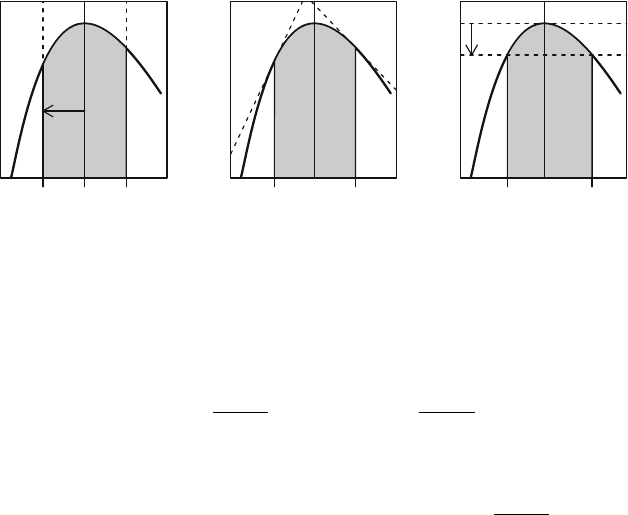
4.11 Confidence Intervals 201
Wald interval
ζ
^
Lower
limit
Upper
limit
Log−likelihood
Score interval
ζ
^
Lower
limit
Upper
limit
Log−likelihood
LR interval
ζ
^
χ
2
q
Lower
limit
Upper
limit
Log−likelihood
Fig. 4.9 Three ways of computing confidence intervals for a one-dimensional situation.
The Wald confidence interval is symmetric by definition; the score and the likelihood
ratio confidence intervals are not necessarily symmetric (Sect. 4.11)
For a single parameter, the approximate 100(1 −α)% confidence interval
based on the Wald statistic is obtained directly from (4.27):
ˆ
ζ
j
− z
∗
var[
ˆ
ζ
j
] <ζ
j
<
ˆ
ζ
j
+ z
∗
var[
ˆ
ζ
j
]
where z
∗
is the quantile of the standard normal distribution such that an area
α/2 is in each tail. Wald confidence intervals are most commonly used, be-
cause this explicit solution is available, and because
ˆ
ζ
j
and
var[
ˆ
ζ
j
] are found
directly from the fitting algorithm (Sect. 4.8). Note the confidence interval is
necessarily symmetric for the Wald statistic.
Confidence intervals for single parameters based on the score and likeli-
hood statistics are harder to find, as they require numerically solving the
corresponding equations that come from the relevant statistics. The limits of
the confidence interval are the two solutions to
Score: U(ζ)
2
/I(ζ) ≤ χ
2
1,1−α
(4.31)
Likelihood ratio: 2
$
(
ˆ
ζ; y) − (ζ; y)
%
≤ χ
2
1,1−α
(4.32)
Example 4.21. Consider the model fitted to the Quilpie rainfall data (data
file: quiplie)usingsoi as an explanatory variable (Example 4.6,p.174),
and finding a confidence interval for β
1
. The log-likelihood evaluated at the
mlesofβ
0
and β
1
is (
ˆ
β
0
,
ˆ
β
1
; y)=−37.95 and χ
2
1,1−α
=3.841 for a 95%
confidence interval. Then, from (4.30), the limits of the confidence interval
are the two solutions to
2
$
−37.95 − (
ˆ
β
0
,β
1
; y)
%
=3.841, (4.33)

202 4 Beyond Linear Regression: The Method of Maximum Likelihood
Tabl e 4. 6 Confidence intervals for β
1
, using the Wald, score and likelihood ratio statis-
tics. Note that
ˆ
β
1
=0.1464 (Sect. 4.11)
Type of interval Lower Upper
Wald: 0.06238 0.2305
Score: 0.06552 0.2289
Likelihood-ratio: 0.07191 0.2425
a non-linear equation which must be solved numerically. One solution will be
less than
ˆ
β
1
=0.1464, and one solution greater than
ˆ
β
1
=0.1464.
In Fig. 4.9, confidence intervals are shown based on the Wald, score and
likelihood-ratio statistics. The Wald confidence interval is symmetric, by def-
inition. The confidence intervals based on the score and log-likelihood func-
tions are not necessarily symmetric (Table 4.6), since the log-likelihood func-
tion is not exactly symmetric about
ˆ
β
1
.
4.12 Comparing Non-nested Models: The AIC and BIC
In Sect. 2.11,theaic and bic were used to compare non-nested linear regres-
sion models. More generally, the aic and bic can be used to compare any
non-nested models based on a specific probability distribution, by using the
log-likelihood and penalizing the complexity of models. Formally, the aic is
defined [1] in terms of the log-likelihood as
aic = −2(
ˆ
ζ
1
,...,
ˆ
ζ
p
; y)+
2 × (Number of unknown parameters), (4.34)
where (
ˆ
ζ
1
,...,
ˆ
ζ
p
; y) is the log-likelihood evaluated at the mles for the model
under consideration. The aic penalizes the log-likelihood by the number of
unknown parameters using k = 2. Using this definition, smaller values of the
aic (closer to −∞) represent better models.
Similarly, the bic is defined as
bic = −2(
ˆ
ζ
1
,...,
ˆ
ζ
p
; y)+
(log n) × (Number of unknown parameters). (4.35)
The bic penalizes the log-likelihood by the number of unknown parameters
using k = 2 log n. The results in Sect 2.11 (p. 70) are simply those for (4.34)
and (4.35) applied to normal linear regression models (Problem 4.10), ignor-
ing all constants.
4.12 Comparing Non-nested Models: The AIC and BIC 203
Example 4.22. Consider the model quilpie.m1 fitted to the Quilpie rainfall
data quiplie in Example 4.15 (p. 187). The aic and bic are:
> LLH <- m1.quilpie$LLH
> m1.aic <- -2 * LLH+2*length(m1.quilpie$coef)
> m1.bic <- -2 * LLH + log(length(quilpie$y)) * length(m1.quilpie$coef)
> c(AIC=m1.aic, BIC=m1.bic)
AIC BIC
79.90060 84.33962
Rather than using the soi as an explanatory variable, an alternative is to
use the soi phases [14]. The soi can be classified into one of five phases,
depending on the soi in the current and previous months (see ?quilpie for
more details). For five soi phases, four dummy variables are needed, so the
total number of estimated parameters is five (including the constant). The
fitted model is:
> quilpie$Phase <- factor( quilpie$Phase )
> Xvars <- with( quilpie, model.matrix( ~ Phase))#Create dummy vars
> head(Xvars)
(Intercept) Phase2 Phase3 Phase4 Phase5
1 11000
2 10001
3 10100
4 11000
5 10100
6 10010
> phase.quilpie <- FitModelMle(quilpie$y, x=Xvars, add.constant=FALSE )
(Notice the use of model.matrix() to automatically define the dummy vari-
ables for soi phases.) The two models m1.quilpie and phase.quilpie are
not nested, so comparing the models using the likelihood ratio test is inap-
propriate. Instead, the aic and bic are:
> LLH <- phase.quilpie$LLH
> m2.aic <- -2 * LLH+2*length(phase.quilpie$coef)
> m2.bic <- -2 * LLH + log(length(quilpie$y)) * length(phase.quilpie$coef)
> c( "AIC (SOI model)"=m1.aic, "AIC (SOI Phase model)"=m2.aic)
AIC (SOI model) AIC (SOI Phase model)
79.90060 75.79902
> c( "BIC (SOI model)"=m1.bic, "BIC (SOI Phase model)"=m2.bic)
BIC (SOI model) BIC (SOI Phase model)
84.33962 86.89656
The aic suggests that the model using the soi phases makes better predic-
tions than using the soi,astheaic for the soi model is closer to −∞.In
contrast, the bic suggests that the model using the soi is a superior model.
204 4 Beyond Linear Regression: The Method of Maximum Likelihood
4.13 Summary
Chapter 4 discusses situations where linear regression models do not apply,
and explores the theory of likelihood methods for estimation in these contexts.
We considered three important cases for which linear regression models
fail (Sect. 4.2):
• The response y is a proportion of a total number of counts, where 0 ≤
y ≤ 1.
• The response y is a count, where y =0, 1, 2,....
• The response y is positive continuous, where y>0.
A more general approach to regression models assumes the responses belong
to a family of distributions (Sect. 4.3).
For these models, maximum likelihood methods (Sect. 4.4) can be used for
estimation and hypothesis testing. We consider the one parameter (Sect. 4.5)
and two-parameter (Sect. 4.6) cases separately, and then the case of many
parameters using matrix algebra (Sect. 4.7).
Estimation using maximum likelihood includes a discussion of the score
equations (Sect. 4.5.1) the observed and expected information (Sect. 4.5.2)
and standard errors (Sect. 4.5.3). Then, the Fisher scoring algorithm for find-
ing the maximum likelihood estimates was detailed (Sect. 4.8). Maximum
likelihood estimators are invariant, asymptotically unbiased, asymptotically
efficient, consistent, and asymptotically normally distributed (Sect. 4.9).
Three types of inference are suggested by maximum likelihood methods:
Wald, score and likelihood ratio (Sect. 4.10 for hypothesis testing;. Sect. 4.11
for confidence intervals). Asymptotic results are available for describing the
distribution of the Wald, score and likelihood ratio statistics, which apply as
n →∞(Sect. 4.10). Non-nested models can be compared using the aic or
the bic (Sect. 4.12).
* 4.14 Appendix: R Code to Fit Models to the Quilpie
Rainfall Data
In Example 4.15 (p. 187), a model was fitted to the Quilpie rainfall data using
the ideas in Sect. 4.8 (p. 186). The r code used to fit these models is shown
below. The purpose of the code is to demonstrate the application of the ideas
and formulae, and is not optimal r programming (for example, there is no
error checking). Later (Chap. 6), built-in r functions are described to fit these
models without the need to use these functions. Notes on writing r functions
are given in Sect. A.3.11.
# Function for computing the information matrix:
MakeExpInf <- function(x, mu){
# Args:
4.14 Appendix: R Code to Fit Models to the Quilpie Rainfall Data 205
# x: The matrix of explanatory variables
# mu: The fitted values
#
# Returns:
# The expected information matrix
if ( length(mu) ==1)mu<-rep( mu, dim(x)[1])
mu <- as.vector(mu)
return( t(x) %*% diag( mu * (1 - mu) ) %*% x )
}
# Function for computing mu:
MakeMu <- function(x, beta){
# Args:
# x: The matrix of explanatory variables
# beta: The linear model parameter estimates
#
# Returns:
# The value of mu
eta <- x %*% beta
return(1/(1+exp( -eta)))
}
# Function for computing the score vector:
MakeScore <- function(x, y, beta){
# Args:
# x: The matrix of explanatory variables
# y: The response variable
# beta: The linear model parameter estimates
#
# Returns:
# The score matrix
mu <- MakeMu(x, beta)
return( t(x) %*% (y - mu) )
}
FitModelMle <- function(y, x=NULL, maxits=8, add.constant=TRUE){
# Args:
# y: The response variable
# x: The matrix of explanatory variables
# maxits: The maximum number of iteration for the algorithm
# add.constant: If TRUE, a constant is added to the x matrix
# (All models must have a constant term.)
#
# Returns:
# Information about the fitted glm
if ( is.null(x)){ # If no x given, ensure constant appears
allx <- cbind( Constant=rep( 1, length(y) ) )
} else {
allx <- x
if( add.constant ){
allx <- cbind( Constant=rep(1, length(y)), x)
}
}
num.x.vars <- dim(allx)[2] - 1 # Take one, because of constant
# Find initials: beta_0 = mean(y), and the other beta_j are zero
beta <- c( mean(y), rep( 0, num.x.vars ) )
206 4 Beyond Linear Regression: The Method of Maximum Likelihood
# Set up
beta.vec <- array( dim=c(maxits, length(beta) ) )
beta.vec[1,] <- beta
mu <- MakeMu( allx, beta )
score.vec <- MakeScore(allx, y, beta)
inf.mat <- MakeExpInf( allx, mu )
# Now iterate to update
for (i in (2:maxits)){
beta <- beta + solve( inf.mat ) %*% score.vec
beta.vec[i,] <- beta
mu <- MakeMu( allx, beta )
score.vec <- MakeScore(allx, y, beta)
inf.mat <- MakeExpInf( allx, mu )
}
# Compute log-likelihood
LLH <- sum( y*log(mu) + (1-y)*log(1-mu) )
return( list(coef = beta.vec[maxits,], # MLE of parameter estimates
coef.vec = beta.vec, # Estimates at each iteration
LLH = LLH, # The maximum log-likelihood
inf.mat = inf.mat, # The information matrix
score.vec = score.vec, # The score vector
mu = mu) ) # The fitted values
}
Problems
Selected solutions begin on p. 534. Problems preceded by an asterisk * refer
to the optional sections in the text, and may require matrix manipulations.
4.1. Show that an approximation to the Wald statistic can be developed from
the second-order Taylor expansion of the log-likelihood as follows. For this
problem, focus on just one of the regression parameters, say β
j
.
1. Write the first three terms of the Taylor series expansion of (β
j
; y)ex-
panded about
ˆ
β
j
.
2. Rearrange to show that the Wald statistic is approximately equal to
2{(β
j
; y) −(
ˆ
β
j
; y)}, and hence show that the Wald statistic is approxi-
mately equivalent to a likelihood ratio test when β
j
−
ˆ
β
j
is small.
*4.2.In Example 4.10 (p. 180), the information matrix was given for the
Bernoulli model fitted to the Quilpie rainfall data. Prove the result in (4.15).
*4.3.In Sect. 4.7.3 (p. 184), two statements were made concerning the log-
likelihood, which we now prove. In this question, assume y is continuous.

4.14 Appendix: r Code to Fit Models to the Quilpie Rainfall Data 207
1. Working with just one observation, use the definition of the expected
value to show that
E[U(ζ)] =
&
∞
−∞
∂P(y; ζ)
∂ζ
dy. (4.36)
Then use (4.36)toshowthatE[U(ζ)] = 0.
2. Using that E[U (ζ)] = 0 and the definition of the variance, show that
var[U(ζ)] = E[U (ζ)U(ζ)
T
], which is I(ζ) (assuming the order of the
integration and differentiation can be reversed).
4.4. The normal distribution N(μ, σ
2
) has the probability function
P(y; μ, σ
2
)=
1
√
2πσ
2
exp
−
(y −μ)
2
2σ
2
,
for σ>0, −∞ <μ<∞ and −∞ <y<∞. Consider estimating the mean μ
for the normal distribution when σ
2
is known, based on a sample y
1
,...,y
n
.
1. Determine the likelihood function and the log-likelihood function.
2. Find the score function.
3. Using the score function, find the mle of μ.
4. Find the observed and expected information for μ.
5. Find the standard error for ˆμ.
6. Find the Wald test statistic W for testing H
0
: μ =0.
7. Find the score test statistic S for testing H
0
: μ =0.
8. Find the likelihood ratio test statistic L for testing H
0
: μ =0.
9. Show that W = S = L in this example.
4.5. The exponential distribution has the probability function
P(y; μ) = exp(−y/μ)/μ, (4.37)
for μ>0andy>0. Consider estimating the mean μ for the exponential
distribution based on a sample y
1
,...,y
n
.
1. Determine the likelihood function and the log-likelihood function.
2. Find the score function.
3. Using the score function, find the mle of μ.
4. Find the observed and expected information for μ.
5. Show that the standard error for ˆμ is se(ˆμ)=ˆμ/
√
n.
6. Show that the Wald test statistic for testing H
0
: μ =1isW =(ˆμ −
1)
2
/(ˆμ
2
/n).
7. Show that the score test statistic for testing H
0
: μ =1isS = n(ˆμ − 1)
2
.
8. Show that the likelihood ratio test statistic for testing H
0
: μ =1is
L =2n(ˆμ − log ˆμ − 1).
9. Plot W , S and L for values of μ between 0.5 and 2, for n = 10. Comment.
10. Plot W, S and L for values of μ between 0.5 and 2, for n = 100. Comment.

208 4 Beyond Linear Regression: The Method of Maximum Likelihood
4.6. Use the r function rexp() to generate n = 100 random numbers from
the exponential distribution (4.37) with μ =1.(Inr, the parameter of the
exponential distribution is the rate where the rate is 1/μ.)
1. Use r to plot the likelihood function for the randomly generated data
from μ =0.75 to μ =1.25. Use vertical lines to show the location of ˆμ
and μ
0
=1.
2. Test the hypothesis H
0
: μ = 1 using the Wald, score and likelihood ratio
statistics developed in Problem 4.5.
3. Plot the Wald, score and likelihood ratio test statistics against possible
values of μ. Use a horizontal line to show the location of the critical value
of χ
2
1
. Compare the values of the test statistics for various values of ˆμ.
4. Find the standard error of ˆμ.
5. Find a 95% confidence interval for μ using the Wald statistic.
*4.7.Consider a model based on the exponential distribution (4.37), where
log μ = β
0
+ β
1
x. Consider estimating the regression parameters based on a
sample y
1
,...,y
n
.
1. Show that the score vector has elements
∂
∂β
0
=
n
i=1
y
i
− μ
i
μ
i
and
∂
∂β
1
=
n
i=1
(y
i
− μ
i
)x
i
μ
i
.
2. Show that the second derivatives of the log-likelihood are
∂
2
∂β
2
0
= −
n
i=1
y
i
μ
i
;
∂
2
∂β
2
1
= −
n
i=1
y
i
x
2
i
μ
i
;
∂
2
∂β
0
∂β
1
= −
n
i=1
y
i
x
i
μ
i
.
3. Using the results above, determine an expression for se(
ˆ
β
1
).
4. Define the Wald test statistic for testing H
0
: β
1
=0.
4.8. The Poisson distribution has the probability function
P(y; μ)=
exp(−μ)μ
y
y!
,
for μ>∞ and where y is a non-negative integer. Initially, consider estimating
the mean μ for the Poisson distribution, based on a sample y
1
,...,y
n
.
1. Determine the likelihood function and the log-likelihood function.
2. Find the score function U (μ).
3. Using the score function, find the mle of μ.
4. Find the observed and expected information for μ.
5. Find the standard error for ˆμ.
*4.9.Following Problem 4.8, now consider the case where log μ = β
0
+ β
1
x.
1. Find the score functions U (β
0
)andU(β
1
).
REFERENCES 209
2. Find the observed and expected information matrices.
3. Hence find the standard errors of β
0
and β
1
.
4.10. Using the definition of the aic in (4.34), show that the formulae for
computing the aic in normal linear regression models is given by aic =
n log(rss/n)+2p
, as shown in (2.35)(p.71), after ignoring all constants.
References
[1] Akaike, H.: A new look at the statistical model identification. IEEE
Transactions on Automatic Control 19(6), 716–723 (1974)
[2] Box, G.E.P.: Science and statistics. Journal of the American Statistical
Association 71, 791–799 (1976)
[3] Chatterjee, S., Handcock, M.S., Simonoff, J.S.: A Casebook for a First
Course in Statistics and Data Analysis. John Wiley and Sons, New York
(1995)
[4] Dala, S.R., Fowlkes, E.B., Hoadley, B.: Risk analysis of the space shuttle:
pre-Challenger prediction of failure. Journal of the American Statistical
Association 84(408), 945–957 (1989)
[5] Dunn, P.K., Smyth, G.K.: Randomized quantile residuals. Journal of
Computational and Graphical Statistics 5(3), 236–244 (1996)
[6] Feigl, P., Zelen, M.: Estimation of exponential survival probabilities with
concomitant information. Biometrics 21, 826–838 (1965)
[7] Glaister, D.H., Miller, N.L.: Cerebral tissue oxygen status and psychomo-
tor performance during lower body negative pressure (LBNP). Aviation,
Space and Environmental Medicine 61(2), 99–105 (1990)
[8] Hauck Jr., W.W., Donner, A.: Wald’s test as applied to hypotheses in
logit analysis. Journal of the American Statistical Association 72, 851–
853 (1977)
[9] Maron, M.: Threshold effect of eucalypt density on an aggressive avian
competitor. Biological Conservation 136, 100–107 (2007)
[10] McBride, J.L., Nicholls, N.: Seasonal relationships between Australian
rainfall and the southern oscillation. Monthly Weather Review 111(10),
1998–2004 (1983)
[11] Montgomery, D.C., Peck, E.A.: Introduction to Regression Analysis. Wi-
ley, New York (1992)
[12] Pook, M., Lisson, S., Risbey, J., Ummenhofer, C.C., McIntosh, P.,
Rebbeck, M.: The autumn break for cropping in southeast Australia:
trends, synoptic influences and impacts on wheat yield. International
Journal of Climatology 29, 2012–2026 (2009)
[13] Smyth, G.K.: Australasian data and story library (Ozdasl) (2011).
URL http://www.statsci.org/data
[14] Stone, R.C., Auliciems, A.: soi phase relationships with rainfall in east-
ern Australia. International Journal of Climatology 12, 625–636 (1992)

Chapter 5
Generalized Linear Models:
Structure
Models are useful distillations of reality. Although wrong
by definition, they are the wind that blows away the fog
and cuts through the untamed masses of data to let us see
answers to our questions.
Kel ler [4, p. 97]
5.1 Introduction and Overview
Chapters 2 and 3 considered linear regression models. These models assume
constant variance, which demonstrably is not true for all data, as shown
in Chap. 4. Generalized linear models (glms) assume the responses come
from a distribution that belongs to a more general family of distributions,
and also permit more general systematic components. We first review the
two components of a glm (Sect. 5.2) then discuss in greater detail the fam-
ily of distributions upon which the random component is based (Sect. 5.3),
including writing the probability functions in the useful dispersion model
form (Sect. 5.4). The systematic component of the glm is then considered in
greater detail (Sect. 5.5). Having discussed the two components of the glm,
glms are then formally defined (Sect. 5.6), and the important concept of the
deviance function is introduced (Sect. 5.7). Finally, using a glm is compared
to using a regression model after transforming the response (Sect. 5.8).
5.2 The Two Components of Generalized Linear Models
Generalized linear models (glms) are regression models (Sect. 1.6), and so
consist of a random component and a systematic component. The random
and systematic components take specific forms for glms, which depend on
the answers to the following questions:
1. What probability distribution is appropriate? The answer determines the
random component of the model. The choice of probability distribution
may be suggested by the response data (for example, proportions of a
total suggest a binomial distribution), or knowledge of how the variance
changes with the mean.
© Springer Science+Business Media, LLC, part of Springer Nature 2018
P. K. Dunn, G. K. Smyth, Generalized Linear Models with Examples in R,
Springer Texts in Statistics, https://doi.org/10.1007/978-1-4419-0118-7_5
211

212 5 Generalized Linear Models: Structure
2. How are the explanatory variables related to the mean of the response
μ? The answer suggests the systematic component of the model. Glms
assume a function linking the linear predictor η = β
0
+
p
j=1
β
j
x
j
to
the mean μ, such as log μ = η for example. That is, glms are regression
models linear in the parameters.
5.3 The Random Component: Exponential Dispersion
Models
5.3.1 Examples of EDMs
Glms assume the responses come from a distribution that belongs to a fam-
ily of distributions called the exponential dispersion model family (or edm
family, or just edms). Continuous edms include the normal and gamma dis-
tributions. Discrete edms include the Poisson, binomial and negative bino-
mial distributions. The edm family of distributions enables glms to be fitted
to a wide range of data types, including binary data (Chap. 4), proportions
(Chap. 9), counts (Chap. 10), positive continuous data (Chap. 11), and posi-
tive continuous data with exact zeros (Chap. 12).
5.3.2 Definition of EDMs
Distributions in the edm family have a probability function (a probability
density function if y is continuous; a probability mass function if y is discrete)
of the form
P(y; θ, φ)=a(y,φ)exp
yθ − κ(θ)
φ
(5.1)
where
• θ is called the canonical parameter.
• κ(θ) is a known function, and is called the cumulant function.
• φ>0isthedispersion parameter.
• a(y,φ) is a normalizing function ensuring that (5.1) is a probability
function. That is, a(y, φ) is the function of φ and y ensuring that
'
P(y; θ, φ) dy = 1 over the appropriate range if y is continuous, or the
function ensuring that
y
P(y; θ, φ) dy =1ify is discrete. The function
a(y, φ) cannot always be written in closed form.
The mean μ is a known function of the canonical parameter θ (Sect. 5.3.5).
The notation y ∼ edm(μ, φ) indicates that the responses come from a dis-
tribution in the edm family (5.1), with mean μ and dispersion parameter
φ. Definition (5.1) writes the form of an edm in canonical form. Other pa-
rameterizations are also possible, and the dispersion model form (Sect. 5.4)
is particularly important.

5.3 The Random Component: Exponential Dispersion Models 213
The support of y (the set of possible values for y) is denoted by S, where
S does not depend on the parameters θ and φ. The domain of θ, denoted
Θ, is an open interval of values satisfying κ(θ) < ∞ that includes zero. The
corresponding domain of μ is denoted Ω.
Example 5.1. The probability density function for the normal distribution
with mean μ and variance σ
2
is
P(y; μ, σ
2
)=
1
√
2πσ
2
exp
−
(y −μ)
2
2σ
2
(5.2)
=
1
√
2πσ
2
exp
yμ −(μ
2
/2)
σ
2
−
y
2
2σ
2
.
Comparing to (5.1), θ = μ is the canonical parameter, κ(θ)=μ
2
/2=θ
2
/2
is the cumulant function, φ = σ
2
is the dispersion parameter, and a(y, φ)=
(2πσ
2
)
−1/2
exp{−y
2
/(2σ
2
)} is the normalizing function. The normal distri-
bution is an edm.
Example 5.2. The Poisson probability function is usually written
P(y; μ)=
exp(−μ)μ
y
y!
for μ>0andy =0,1,2,....Intheformof(5.1),
P(y; μ) = exp{y log μ − μ − log(y!)},
showing that θ = log μ is the canonical parameter, κ(θ)=μ,andφ =1.
The normalizing function is a(y, φ)=1/y!. The Poisson distribution is an
edm.
Example 5.3. The binomial probability function is
P(y; μ, m)=
m
my
μ
y
(1 − μ)
m(1−y)
=
m
my
exp
m
y log
μ
1 − μ
+ log(1 − μ)
, (5.3)
where y =0, 1/m, 2/m,...1, and 0 <μ<1. Comparing to (5.1), θ =
log{μ/(1 −μ)} is the canonical parameter, κ(θ)=−log(1 −μ), φ =1/m and
a(y, φ)=
m
my
. The binomial distribution is an edm when m is known.
Example 5.4. The Weibull distribution has the probability function
P(y; α, γ)=
α
γ
y
γ
α−1
exp
−
y
γ
α

214 5 Generalized Linear Models: Structure
for y>0 with α>0andγ>0. Rewriting,
P(y; α, γ) = exp
−
y
γ
α
+ log
α
γ
+(α − 1) log
y
γ
.
Inside the exponential function, a term of the form yθ cannot be extracted
unless α = 1. Hence, the Weibull distribution is not an edm in general. When
α = 1, the probability function is
P(y; γ) = exp(−y/γ)/γ =exp{−(y/γ) − log γ},
which is the exponential distribution (4.37) with mean γ. The exponential
distribution written in this form is an edm where θ = −1/γ is the canonical
parameter, κ(θ) = log γ and φ =1.
5.3.3 Generating Functions
edms have many important and useful properties. One useful property is that
the moment generating function (mgf) always has a simple form, even if the
probability function cannot be written in closed form. The mean and variance
may be found from this simple mgf.
The moment generating function, denoted M (t), for some variable y with
probability function P(y)is
M(t)=E[e
ty
]=
⎧
⎪
⎪
⎨
⎪
⎪
⎩
&
S
P(y)e
ty
dy for y continuous
y∈S
P(y)e
ty
for y discrete,
for all values of t for which the expectation exists. The cumulant generating
function (or cgf) is then defined as
K(t) = log M(t) = log E[e
ty
],
for all values of t for which the expectation exists. The cgf is used to derive
the cumulants of a distribution, such as the mean (first cumulant, κ
1
)and
the variance (second cumulant, κ
2
). The rth cumulant, κ
r
,is
κ
r
=
d
r
K(t)
dt
r
(
(
(
(
t=0
(5.4)

5.3 The Random Component: Exponential Dispersion Models 215
where the notation means to evaluate the indicated derivative at t =0.Using
the cgf, the mean and variance are (Problem 5.4):
E[y]=κ
1
=
dK(t)
dt
(
(
(
(
t=0
and var[y]=κ
2
=
d
2
K(t)
dt
2
(
(
(
(
t=0
. (5.5)
5.3.4 The Moment Generating and Cumulant
Functions for EDMs
The mgf, and hence cgf, for an edm has a very simple form. The mgf is
developed here for a continuous response, but the results also hold for discrete
distributions (Problem 5.6).
Using (5.1), the mgf for an edm is
M(t) = E[exp(ty)]
=
&
S
exp(ty)a(y,φ)exp
yθ − κ(θ)
φ
dy
=exp
κ(θ
) − κ(θ)
φ
&
S
a(y, φ)exp
yθ
− κ(θ
)
φ
dy,
where θ
= θ + tφ. The integral on the right is one, since the integrand is an
edm density function (5.1) written in terms of θ
rather than θ. This means
that the mgf and cumulant generating function (cgf) for an edm are
M(t) = exp
κ(θ + tφ) − κ(θ)
φ
; (5.6)
K(t)=
κ(θ + tφ) − κ(θ)
φ
. (5.7)
Using (5.7), the rth cumulant for an edm is (Problem 5.5)
κ
r
= φ
r−1
d
r
κ(θ)
dθ
r
. (5.8)
For this reason, κ(θ) is called the cumulant function.
Example 5.5. For the normal distribution, the results in Example 5.1 can be
used with (5.7) to obtain
K(t)=
(μ + tσ
2
)
2
2σ
2
−
μ
2
2σ
2
= μt +
σ
2
t
2
2
.

216 5 Generalized Linear Models: Structure
Example 5.6. For the Poisson distribution, the results in Example 5.2 can be
used to obtain K(t)=μ(exp t − 1).
5.3.5 The Mean and Variance of an EDM
The mean and variance of an edm are found by applying (5.8)to(5.5):
E[y]=μ =
dκ(θ)
dθ
and var[y]=φ
d
2
κ(θ)
dθ
2
. (5.9)
Observe that
d
2
κ(θ)
dθ
2
=
d
dθ
dκ(θ)
dθ
=
dμ
dθ
.
Since d
2
κ(θ)/dθ
2
> 0 is a variance, then dμ/dθ>0. This means that μ
must be a monotonically increasing function of θ,soμ and θ are one-to-one
functions of each other. Hence, define
V (μ)=
dμ
dθ
, (5.10)
called the variance function. Then the variance of y can be written as
var[y]=φV (μ). (5.11)
The variance is a product of the dispersion parameter φ and V (μ). Table 5.1
(p. 221) gives the variance function for common edms.
Example 5.7. For the normal distribution (Example 5.1; Table 5.1), κ(θ)=
θ
2
/2, and so E[y]=dκ(θ)/dθ = θ. Since θ = μ for the normal distribution,
E[y]=θ = μ (as expected). For the variance, compute V (μ)=d
2
κ(θ)/dθ
2
=
1, and so var[y]=φV (μ)=σ
2
as expected.
Example 5.8. For the Poisson distribution (Example 5.2; Table 5.1), κ(θ)=μ
and θ = log μ. The mean is
E[y]=
dκ
dθ
=
dκ
dμ
×
dμ
dθ
= μ
as expected. For the variance function, V (μ)=dμ/dθ = μ. Since φ =1for
the Poisson distribution, var[y]=μ for the Poisson distribution.

5.3 The Random Component: Exponential Dispersion Models 217
5.3.6 The Variance Function
The variance function V (μ) uniquely determines the distribution within the
class of edms since the variance function determines κ(θ), up to an addi-
tive constant. This in turn specifies K(t), which uniquely characterizes the
distribution.
To demonstrate, consider edms with V (μ)=μ
2
. Since V (μ)=dμ/dθ
from (5.10), solve dθ/dμ = μ
−2
for θ to obtain θ = −1/μ, setting the inte-
gration constant to zero. Then using that μ =dκ(θ)/dθ from (5.9) together
with θ = −1/μ shows that κ(θ)=−log(−θ) = log μ. Using these forms for θ
and κ(θ), the edm uniquely corresponding to V (μ)=μ
2
has the probability
function
P(y)=a(y, φ)exp
y(−1/μ) − log μ
φ
,
for an appropriate normalizing function a(y; φ). The constants of integra-
tion are not functions of μ, so are absorbed into a(y, φ) if not set to zero.
This probability function is the probability function for a gamma distribu-
tion. Hence, the variance function V (μ)=μ
2
uniquely refers to a gamma
distribution within the edm class of distributions.
This result means that if the mean–variance relationship can be estab-
lished for a given data set, and quantified using the variance function, the
corresponding edm is uniquely identified.
In general, (5.11) states that, in general, the variance of an edm depends
on the mean. The normal distribution is unique in the family of edms, as its
variance does not depend on the mean since V (μ) = 1. For other edms, the
variance is a function of the mean, and the role of the variance function is to
specify exactly that function.
Example 5.9. For the noisy miner data [6] in Table 1.2 (data set: nminer),
divide the data into five approximately equal-sized groups:
> data(nminer)
> breaks <- c(-Inf, 4, 11, 15, 19, Inf) + 0.5 # Break points
> Eucs.cut <- cut(nminer$Eucs, breaks ); summary(Eucs.cut)
(-Inf,4.5] (4.5,11.5] (11.5,15.5] (15.5,19.5] (19.5, Inf]
96565
For each group, compute the mean and variance of the number of noisy
miners:
> mn <- tapply( nminer$Minerab, Eucs.cut, "mean" ) # Mean of each group
> vr <- tapply( nminer$Minerab, Eucs.cut, "var" ) # Var of each group
> sz <- tapply( nminer$Minerab, Eucs.cut, "length" ) # Num. in each group
> cbind("Group size"=sz, "Group mean"=mn, "Group variance"=vr)
Group size Group mean Group variance
(-Inf,4.5] 9 0.1111111 0.1111111
(4.5,11.5] 6 0.5000000 1.5000000
(11.5,15.5] 5 3.8000000 11.2000000
218 5 Generalized Linear Models: Structure
(15.5,19.5] 6 4.3333333 7.8666667
(19.5, Inf] 5 7.0000000 48.5000000
The command tapply(nminer$Minerab, Eucs.cut, "mean") computes
the mean() of nminer$Minerab for each level of Eucs.cut. More generally,
tapply(X, INDEX, FUN) applies the function FUN() to the data X,foreach
group of values in the unique combination of factors in INDEX.
A plot of the logarithm of each group mean against the logarithm of each
group variance (Fig. 5.1, right panel) shows that, in general, the variance
increases as the mean increases:
> plot(jitter(Minerab)~(Eucs), pch=1, las=1, data=nminer, ylim=c(0, 20),
xlab="Number of eucalypts/2 ha.", ylab="Number of noisy miners")
> # Draw the dashed vertical lines
> abline(v=breaks, lwd=1, lty=2, col="gray")
> plot( log( vr ) ~ log ( mn ), pch=19, las=1, cex=0.45*sqrt(sz),
xlab="Log of means", ylab="Log of variances" )
(The points are plotted so that the area is proportional to the sample size.
The scaling factor 0.45 is chosen by trial-and-error.) More specifically, an
approximate linear a relationship of the form
log(group variance) = a + b log(group mean)
may be reasonable (Fig. 5.1, right panel). This is equivalent to (group
variance) ∝ (group mean)
b
. This is the form of the variance of an edm:
var[y]=φV (μ), where V (μ)=μ
b
and where b is the slope of the linear
relationship:
> hm.lm <- lm( log( vr ) ~ log ( mn ), weights=sz )
> coef(hm.lm); confint(hm.lm)
(Intercept) log(mn)
0.802508 1.295222
2.5 % 97.5 %
(Intercept) 0.007812159 1.597204
log(mn) 0.821058278 1.769386
For the data, the slope of the linear regression line (weighted by the number
of observations in each group) is b ≈ 1.3, suggesting the mean is approxi-
mately proportional to the variance. In addition, the estimate of φ is approx-
imately 1 as needed for the Poisson distribution. In other words, V (μ)=μ
approximately. Since this is the variance function for a Poisson distribution
(Table 5.1), a Poisson distribution may be suitable for the data. Of course,
the Poisson distribution is also suggested because the data are counts.
5.4 EDMs in Dispersion Model Form
5.4.1 The Unit Deviance and the Dispersion Model Form
We have shown that μ and θ are one-to-one functions of each another. As a
result, it must be possible to write the probability function (5.1) as a function

5.4 EDMs in Dispersion Model Form 219
l
l
l
l
l
l
l
l
l
l
l
l
l
l
l
l
l
l
l
l
l
l
l
l
l
l
l
l
l
l
l
0 5 10 15 20 25 30
0
5
10
15
20
Number of eucalypts/2 ha.
Number of noisy miners
l
l
l
l
l
−2 −1 0 1 2
−2
−1
0
1
2
3
4
Log of means
Log of variances
Fig. 5.1 Plots of the noisy miner data. Left: the number of noisy miners plotted against
the number of eucalypt trees (a small amount of randomness is added in the vertical
direction to the number of noisy miners to avoid over-plotted observations). The dashed
vertical lines break the data into five groups of similar size. Right panel: the logarithm
of sample variances for each group plotted against the logarithm of the sample means
for each group in the data; the area of the plotted points are proportional to the number
of observations in each group (Example 5.9)
of μ instead of θ. We will see that this version has some advantages because
μ has such a clear interpretation as the mean of the distribution. To do this,
start by writing
t(y, μ)=yθ − κ(θ)
for that part of the probability function which depends on θ. There must be
some function t(·, ·) for which this is true. Now consider t(y, μ) as a function
of μ. See that
∂t(y, μ)
∂θ
= y −
dκ(θ)
dθ
= y −μ
and
∂
2
t(y, μ)
∂θ
2
=
d
2
κ(θ)
dθ
2
= V (μ) > 0.
The second derivative is always positive, and the first derivative is zero at
y = μ,sot(y, μ) must have a unique maximum with respect to μ at μ = y.
This allows us to define a very important quantity, the unit deviance:
d(y, μ)=2{t(y, y) − t(y, μ)}. (5.12)
Notice that d(y, μ) = 0 only when y = μ and otherwise d(y, μ) > 0. In fact,
d(y, μ) increases as μ moves away from y in either direction. This shows that
d(y, μ) can be interpreted as a type of distance measure between y and μ.

220 5 Generalized Linear Models: Structure
In terms of the unit deviance, the probability function (5.1) for an edm is
P(y; μ, φ)=b(y, φ)exp
−
1
2φ
d(y, μ)
, (5.13)
where b(y,φ)=a(y,φ)exp{t(y,y)/φ}, which cannot always be written in
closed form. This is called the dispersion model form of the probability func-
tion for edms, and is invaluable for much of what follows.
Example 5.10. For the normal distribution (Example 5.1), deduce that
t(y, μ)=yμ − μ
2
/2andsot(y,y)=y
2
− y
2
/2=y
2
/2. The unit dev-
iance then is d(y, μ)=(y − μ)
2
. Hence the normal distribution written
as (5.2) is in dispersion model form.
The above definition for the unit deviance assumes that we can always set
μ equal to y. However, cases exist when values of y are not allowable values
for μ. The important cases occur when y is on the boundary of the support of
the distribution. For example, the binomial distribution requires 0 <μ<1,
so setting μ = y is not possible when y =0ory = 1. However μ can still take
values arbitrarily close to y. To cover these cases, we generalize the definition
of the unit deviance to
d(y, μ)=2
$
lim
→0
t(y + , y + ) − t(y, μ)
%
. (5.14)
If y is on the lower boundary of S, the right limit will be taken. If y is at
the upper bound (such as y = 1 for the binomial), then the left limit is
taken. This definition covers all the distributions considered in this book. For
simplicity, the unit deviance is usually written as (5.12), on the understanding
that (5.14) is used when necessary. The unit deviances for common edmsare
in Table 5.1 (p. 221).
Example 5.11. Consider the Poisson distribution in Example 5.2 (p. 213), for
which μ>0. Deduce that t(y, μ)=y log μ − μ.Ify = 0, then t(y, y)=
y log y − y,sothat
d(y, μ)=2
y log
y
μ
− (y − μ)
. (5.15)
If y = 0 we need the limit form (5.14) of the unit deviance instead. It is easily
seen that lim
↓0
t(y + , y + )=0sothat
d(0,μ)=2μ. (5.16)
The unit deviance is commonly written as (5.15) on the understanding that
the limit form (5.16) is used when y = 0. The other terms in the dispersion
model form (5.13)areb(y)=(y log y − y)/y!andφ =1.
As already noted, the unit deviance is a measure of the discrepancy be-
tween y and μ. For normal distributions, the unit deviance d(y, μ)=(y −μ)
2
(Example 5.10) is symmetric about μ as a function of y. For other edms, the

Tabl e 5.1 Common edms, showing their variance function V (μ), cumulant function κ(θ), canonical parameter θ, dispersion parameter φ, unit
deviance d(y, μ), support S (the permissible values of y), domain Ω for μ and domain Θ for θ. For the Tweedie distributions, the case ξ =2is
the gamma distribution, and ξ =1withφ = 1 is the Poisson distribution. R refers to the real line; N refers to the natural numbers 1, 2,...;
superscript + means positive values only; superscript − means negative values only; subscript 0 means zero is included in the space (Sect. 5.3.5)
edm V (μ) κ(θ) θφ d(y, μ) SΩΘReference
Normal 1 θ
2
/2 μσ
2
(y −μ)
2
RRRChaps. 2 and 3
Binomial μ(1 − μ)
exp θ
1+expθ
log
μ
1 − μ
1
m
2
$
y log
y
μ
+(1− y)log
1 − y
1 − μ
%
0, 1,...m
m
(0, 1) R Chap. 9
Negative
binomial μ +
μ
2
k
−log(1 −exp θ)log
μ
μ + k
12
$
y log
y
μ
− (y + k)log
y + k
μ + k
%
N
0
R
+
R
−
Chap. 10
Poisson μ exp θ log μ 12
$
y log
y
μ
− (y −μ)
%
N
0
R
+
R Chap. 10
Gamma μ
2
−log(−θ) −
1
μ
φ 2
$
−log
y
μ
+
y −μ
μ
%
R
+
R
+
R Chap. 11
Inverse
Gaussian μ
3
−
√
−2θ −
1
2μ
2
φ
(y −μ)
2
μ
2
y
R
+
R
+
R
−
0
Chap. 11
Tweedie
(ξ ≤ 0orξ ≥ 1) μ
ξ
{(1 − ξ)θ}
(2−ξ)/(1−ξ)
2 − ξ
μ
1−ξ
1 − ξ
φ 2
max(y, 0)
2−ξ
(1 − ξ)(2 −ξ)
− ξ<0: RR
+
R
+
0
Chap. 12
for ξ =2 forξ =1
yμ
1−ξ
1 − ξ
+
μ
2−ξ
2 − ξ
1 <ξ<2: R
+
0
R
+
R
−
for ξ =1, 2 ξ>2: R
+
R
+
R
−
0

222 5 Generalized Linear Models: Structure
unit deviance is asymmetric (Fig. 5.2), because differences relative to the vari-
ance are important. For example, consider the unit deviance for the gamma
distribution (which has V (μ)=μ
2
) with μ = 3 (Fig. 5.2, bottom left panel).
The unit deviance is greater at y = 1 than at y = 5 even though the absolute
difference |y −μ| = 2 is the same in both cases. This is because the variance
is smaller at y = 1 than at y = 5, so the difference between y and μ is greater
in standard deviation terms.
Technical note. All the edm distributions used for examples in this book
have the property that the domain Ω for μ is the same as the support for y,
at least in a limiting sense. (Technically, the support for y is contained in the
closure of the domain for μ.) However, edms exist for which the allowable
values for μ are far more restricted than those for y. Chapter 12 will discuss
Tweedie models with power variance functions V (μ)=μ
ξ
. When ξ<0, the
resulting distributions can take all values y on the real line, whereas the mean
is restricted to be positive, μ>0. To cover such distributions, the definition
of the unit deviance can be generalized further to
0246
0
1
2
3
4
5
6
Unit deviance for
a normal EDM
The response y
Unit deviance d
(
y
,
μ)
01234567
0
1
2
3
4
5
6
Unit deviance for
a Poisson EDM
The response y
Unit deviance d(y,μ)
l
01234567
0
1
2
3
4
5
6
Unit deviance for
a gamma EDM
The response y
Unit deviance d(
y,
μ
)
Unit deviance for
a binomial EDM
The response y
Unit deviance
d
(y,μ)
0.0 0.2 0.4 0.6 0.8 1.0
0
1
2
3
l
l
Fig. 5.2 The unit deviance d(y, μ)forfouredms. Top left panel: the unit deviance for
the normal distribution when μ = 3; top right panel: the unit deviance for the Poisson
distribution when μ = 3; bottom left panel: the unit deviance for the gamma distribution
when μ =3andφ = 1; bottom right: the unit deviance for the binomial distribution
when μ =0.2. The solid points show where the limit form of the unit deviance (5.14)
has been used (Sect. 5.11)

5.4 EDMs in Dispersion Model Form 223
d(y, μ)=2
sup
μ∈Ω
t(y, μ) − t(y, μ)
(5.17)
where the notation ‘sup’ is short for ‘supremum’. However such distributions
do not have any useful applications for modelling real data, as least not yet,
so we can ignore this technicality in practice. The limiting definition (5.14)
given previously is adequate for all applications considered in this book.
5.4.2 The Saddlepoint Approximation
The saddlepoint approximation to the edm density function P(y; μ, φ) is de-
fined by
˜
P(y; μ, φ)=
1
2πφV (y)
exp
−
d(y, μ)
2φ
. (5.18)
The saddlepoint approximation is often remarkably accurate, even in the
extreme tails of the distribution. As well as being computationally useful
in some cases, the approximation aids our theoretical understanding of the
properties of edms.
For practical use, the term V (y) in the denominator of (5.18) is usually
modified slightly so that it can never take the value zero [7]. For example,
the saddlepoint approximation to the Poisson or negative binomial distribu-
tions can be improved by replacing V (y) with V (y + ) where =1/6. The
saddlepoint approximation, adjusted in this way, has improved accuracy ev-
erywhere as well as having the advantage of being defined at y = 0. This is
called the modified saddlepoint approximation.
Comparing to the dispersion model form (5.13)(p.220), the saddlepoint
approximation (5.18) is equivalent to writing b(y, φ) ≈ 1/
2πφV (y). Ob-
serve that b(y, φ), which for some edms isn’t available in any closed form, is
approximated by a simple analytic function.
Example 5.12. For the normal distribution, V (μ)=1sothatV (y)=1.
Applying (5.18) simply reproduces the probability function for the normal
distribution in dispersion model form (5.2). This shows that the saddlepoint
approximation is exact for the normal distribution.
Example 5.13. For the Poisson distribution, V (μ)=μ so that V (y)=y.The
saddlepoint approximation is therefore
˜
P(y; μ)=
1
√
2πy
exp{−y log(y/μ)+(y −μ)}. (5.19)

224 5 Generalized Linear Models: Structure
5.4.3 The Distribution of the Unit Deviance
The saddlepoint approximation has an important consequence. If the saddle-
point approximation to the probability function of an edm is accurate, then
it follows that the unit deviance d(y, μ) follows a χ
2
1
distribution.
To prove this, we use the fact that the χ
2
1
distribution is determined by
its mgf. Consider a random variable y whose probability function is an edm.
If the saddlepoint approximation to its probability function is accurate, then
the mgf of the unit deviance is
M
d(y,μ)
(t) = E[exp{d(y, μ)t}] (by definition)
=
&
S
exp{d(y, μ)t}
1
2πφV (y)
exp
−
d(y, μ)
2φ
dy.
(Recall that y ∈ S.) Rearranging:
M
d(y,μ)
(t)=
&
S
exp
−d(y, μ)
1 − 2φt
2φ
1
2πφV (y)
dy
=(1− 2φt)
−1/2
&
S
(1 − 2φt)
1/2
{2πφV (y)}
1/2
exp
−d(y, μ)
1 − 2φt
2φ
dy.
Let φ
= φ/(1 − 2φt). Then
M
d(y,μ)
(t)=(1− 2φt)
−1/2
&
S
1
{2πφ
V (y)}
−1/2
exp
−
d(y, μ)
2φ
dy
=(1− 2φt)
−1/2
, (5.20)
since the integrand is the (saddlepoint) density of the distribution with φ
=
φ/(1 − 2φt). The mgf (5.20) identifies a χ
2
1
distribution, showing that
d(y, μ)/φ ∼ χ
2
1
(5.21)
whenever the saddlepoint approximation is accurate. This result forms the
basis of small-dispersion asymptotic theory used in Chap. 7. Note that (5.21)
implies that E[d(y,μ)] = φ whenever the saddlepoint approximation is accu-
rate.
Example 5.14. The saddlepoint approximation is exact for the normal dis-
tribution (Example 5.12), implying that the unit deviance has an exact
χ
2
1
distribution for the normal distribution. The unit deviance for the nor-
mal distribution, found in Example 5.10,isd(y, μ)=(y − μ)
2
. This means
d(y, μ)/φ = {(y − μ)/σ}
2
, which defines a χ
2
1
random variate when y comes
from the N(μ, σ
2
) distribution.

5.4 EDMs in Dispersion Model Form 225
5.4.4 Accuracy of the Saddlepoint Approximation
The saddlepoint approximation is exact for the normal and inverse Gaussian
distributions (Example 5.12; Problem 5.9). For other two-parameter distribu-
tions, the accuracy is such that
˜
P(y; μ, φ)=P(y; μ, φ){1+O(φ)}, where O(φ)
means “order φ”, an expression which is like a constant times φ as φ → 0[3].
This shows that the error is relative, so that the density is approximated
equally well even in the tails of the distribution where the density is low.
This expression also shows that the approximation becomes nearly exact for
φ small.
For the gamma distribution, the saddlepoint approximation is equivalent
to approximating the gamma function Γ (1/φ) in the probability function
with Stirling’s formula
n! ≈ n
n
exp(−n)
√
2πn as n →∞. (5.22)
For the gamma distribution, the relative accuracy of the approximation is
constant for all y.
For the binomial, Poisson and negative binomial distributions, the saddle-
point approximation is equivalent to replacing all factorials in the probability
density functions with their Stirling’s formula equivalents. This means that
the saddlepoint approximation will be good for the Poisson distribution if y is
not too small. For the binomial distribution, the saddlepoint approximation
will be accurate if my and m(1 − y) are both not too small.
Smyth and Verbyla [11] give a guideline for judging when the saddlepoint
approximation is sufficiently accurate to be relied on for practical purposes.
They define
τ =
φV (y)
(y −boundary)
2
, (5.23)
where “boundary” is the nearest boundary of the support S for y. Here τ is
a sort of empirical coefficient of variation. Based on a number of heuristic
and theoretical justifications, they argue that the saddlepoint approxima-
tion should be adequate when τ ≤ 1/3. This corresponds to the following
guidelines (Problems 5.13 to 5.15):
• Binomial distribution: my ≥ 3andm(1 − y) ≥ 3.
• Poisson distribution: y ≥ 3.
• Gamma distribution: φ ≤ 1/3.
These guidelines apply to the ordinary saddlepoint approximation. The mod-
ified saddlepoint approximation is often much better, sometimes adequate for
any y.
Comparing the saddlepoint approximation with the Central Limit Theo-
rem is revealing. It is true that edms converge to normality also as φ → 0,
a result which can be derived from the Central Limit Theorem. However,
the saddlepoint approximation is usually far more accurate, because its error

226 5 Generalized Linear Models: Structure
l
ll
l
l
l
012345
0.00
0.05
0.10
0.15
0.20
0.25
0.30
Prob. function and saddlepoint
approx. for a Poisson EDM
y
Probability
l
Exact
Ordinary
Modified
012345
−2
0
2
4
6
8
Rel. error of saddlepoint
approx. for a Poisson EDM
y
Relative error (%)
Ordinary
Modified
Fig. 5.3 The accuracy of the saddlepoint approximation for the Poisson distribution
with μ =2.Fory = 0 the ordinary saddlepoint approximation is undefined. The modified
saddlepoint is evaluated with =1/6. The accuracy of the modified approximation is
never worse than 2.3% (Example 5.15)
is relative and O(φ), whereas the accuracy of the Central Limit Theorem is
additive and O(
√
φ ). This means that the saddlepoint approximation applies
for larger values of φ than the Central Limit Theorem. For continuous edms,
the saddlepoint approximation holds almost uniformly in the tails of the dis-
tribution, whereas the Central Limit Theorem is best near the mean of the
distribution and deteriorates rapidly in the tails.
Example 5.15. For the Poisson distribution, V (μ)=μ, so the modified sad-
dlepoint approximation is
˜
P(y; μ)=
1
2π(y + )
exp{−y log(y/μ)+(y − μ)}.
The ordinary saddlepoint approximation (5.19) corresponds to =0.Therel-
ative accuracy of the saddlepoint approximation is the same for any μ at given
y (Fig. 5.3, right panel). The relative accuracy of the ordinary approximation
is less than 3% when y ≥ 3. The accuracy of the modified approximation is
excellent, never worse than 2.3%.
5.4.5 Accuracy of the χ
2
1
Distribution for the Unit
Deviance
In the previous section we considered conditions under which the saddlepoint
approximation to the probability function should be accurate. In this section,
5.4 EDMs in Dispersion Model Form 227
we consider what implications this has for the distribution of the unit dev-
iance. We have already noted that the relative accuracy of the saddlepoint
approximation does not depend on μ. However, when we consider the distri-
bution of the unit deviance, the saddlepoint approximation needs to hold for
all likely values of y. So we need μ and φ to be such that values of y close to
the boundary of the distribution are not too likely.
For the normal and inverse Gaussian distributions, the unit deviance has
an exact χ
2
1
distribution since the saddlepoint approximation is exact for
these distributions. For other edms, the distribution of the unit deviance
approaches χ
2
1
for any μ as φ → 0.
We will limit our investigation to considering how close the expected value
of the unit deviance is to its nominal value φ. For continuous distributions,
the expected value of the unit deviance is defined by
E[d(y, μ)] =
&
S
d(y, μ)P(y; μ, φ) dy
where P(y; μ, φ) is the probability density function of the distribution. Using
this expression, the expected value of the unit deviance can be computed for
the gamma distribution, and compared to E[d(y, μ)] = φ (Fig. 5.4, top left
panel). The relative error is less than about 5% provided φ<1/3.
For discrete distributions, the expected value of the unit deviance is defined
by
E[d(y, μ)] =
S
d(y, μ)P(y; μ, φ)
where P(y; μ, φ) is the probability mass function of the distribution. We now
use r to compute the expected value of the unit deviance for the Poisson
distribution, and compare it to its nominal value E[d(y,μ)] = 1 according to
the chi-square approximation (Fig. 5.4, top right panel):
> Poisson.mu <- c(0.000001, 0.001, 0.01, seq(0.1, 10, by=0.1) )
> DensityTimesDeviance <- function(mu) {
y <- seq(0, 100, by=1)
sum( dpois(y, lambda=mu) * poisson()$dev.resids(y, mu, wt=1) )
}
> ExpD.psn <- sapply( Poisson.mu, DensityTimesDeviance)
> plot( ExpD.psn ~ Poisson.mu, las=1, type="n",
main="Poisson distribution", xlab=expression(mu),
ylab="Exp. value of unit deviance")
> polygon( x=c(-1, -1, 12, 12), y=c(0.95, 1.05, 1.05, 0.95),
col="gray", border=NA) # Draws the region of 5% rel. accuracy
> lines( ExpD.psn ~ Poisson.mu, lty=2, lwd=2)
> abline(h=1)
(The awkward construct poisson()$dev.resids() accesses the function
dev.resids() from the poisson() family definition. Despite its name, dev.
resids() returns the unit deviance.) The plots show that the expected value
of the deviance is generally not near one for small μ, but the error is well
below 10% provided μ>3.

228 5 Generalized Linear Models: Structure
For the binomial distribution, plots of the expected value of the deviance
against μ for various values of m (Fig. 5.4, bottom panels) show that the
expected value of the deviance can be far from one when mμ or m(1 −μ)are
small, but the error is reasonable provided mμ > 3andm(1 − μ) > 3.
In summary, the unit deviance is always chi-square for the normal and
inverse Gaussian distributions, and for other common edms the unit deviance
is roughly chi-square with the correct expected value when
• Binomial distribution: mμ ≥ 3andm(1 − μ) ≥ 3.
• Poisson distribution: μ ≥ 3.
• Gamma distribution: φ ≤ 1/3.
0.0 0.1 0.2 0.3 0.4 0.5
0.0
0.1
0.2
0.3
0.4
0.5
Gamma distribution
φ
Exp. value of unit deviance
E[d(y,μ)]
E[d(y,μ)] =φ
0246810
0.0
0.2
0.4
0.6
0.8
1.0
1.2
Poisson distribution
μ
Exp. value of unit deviance
E[d(y,μ)]
E[d(y,μ)] = 1
0.0 0.2 0.4 0.6 0.8 1.0
0.6
0.8
1.0
1.2
1.4
Binomial distribution
μ
Exp. value of unit deviance
m = 2
m = 5
m = 10
0.0 0.2 0.4 0.6 0.8 1.0
0.6
0.8
1.0
1.2
1.4
Binomial distribution
μ
Exp. value of unit deviance
m = 15
m = 30
m = 100
Fig. 5.4 The expected value of the unit deviance (modelled on [12, p. 208]). Top left
panel: the gamma distribution for various values of φ (the solid line represents the target
E[d(y, μ)] = φ); top right panel: the Poisson distribution for various values of μ; bottom
panels: the binomial distribution for various values of μ and m. The gray regions indicate
relative accuracy within 5% (Sect. 5.4.5)
5.5 The Systematic Component 229
5.5 The Systematic Component
5.5.1 Link Function
In addition to assuming that the responses come from the edm family, glms
assume a specific form for the systematic component. Glms assume a sys-
tematic component where the linear predictor
η = β
0
+
p
j=1
β
j
x
j
is linked to the mean μ through a link function g() so that g(μ)=η. This
systematic component shows that glms are regression models linear in the
parameters.
The link function g(·) is a monotonic, differentiable function relating the
fitted values μ to the linear predictor η. Monotonicity ensures that any value
of η is mapped to only one possible value of μ. Differentiability is required for
estimation (Sect. 6.2). The canonical link function is a special link function,
the function g(μ) such that η = θ = g(μ).
Example 5.16. For the normal distribution, θ = μ (Table 5.1,p.221). The
canonical link function is the identity link function g(μ)=μ, which implies
η = μ.
Example 5.17. For the Poisson distribution, θ = log μ (Table 5.1,p.221).
The canonical link function is g(μ) = log μ,sothatlogμ = η. The Poisson
distribution is only defined for positive values of μ, and the logarithmic link
function ensures η (which possibly takes any real value) always maps to a
positive value of
μ. Hence the canonical link function is a sensible link function
to use in this case.
5.5.2 Offsets
In some applications, the linear predictor contains a term that requires no
estimation, which is called an offset. The offset can be viewed as a term β
j
x
ji
in the linear predictor for which β
j
is known a priori. For example, consider
modelling the annual number of hospital births in various cities to facilitate
resource planning. The annual number of births is discrete, so a Poisson
distribution may be appropriate. However, the expected annual number of
births μ
i
in city i depends on the given populations P
i
of the city, since cities
with larger population would be expected to have more births each year, in
230 5 Generalized Linear Models: Structure
general. The number of births per unit of population, assuming a logarithmic
link function, can be modelled using the systematic component
log(μ/P )=η,
for the linear predictor η. Rearranging to model μ:
log(μ) = log P + η.
The first term in the systematic component log P is completely known: noth-
ing needs to be estimated. The term log P is called an offset. Offsets com-
monly appear in Poisson glms, but may appear in any glm (Example 5.18).
The offset variable is commonly a measure of exposure. For example, the
number of cases of a certain disease recorded in various mines depends on the
number of workers, and also on the number of years each worker has worked
in the mine. The exposure would be the number of person-years worked in
each mine, which could be incorporated into a glm as an offset. That is, a
mine with many workers who have been employed for many years would be
exposed to a greater likelihood of a worker contracting the disease than a
mine with only a few workers who have been employed for short periods of
time.
Example 5.18. For the cherry tree data (Example 3.14,p.125), approximat-
ing the shape of the trees as a cone or as a cylinder leads to a model with
the systematic component
log μ = β
0
+ 2 log g + log h, (5.24)
where g is the girth and h is the height of each tree, and the value of β
0
is
different for cones and cylinders. To fit this model, the term 2 log g + log h is
an offset, as this expression has no terms requiring estimation.
5.6 Generalized Linear Models Defined
The two components of a generalized linear model (glm) have been discussed:
the random component (Sect. 5.3) and the systematic component (Sect. 5.5).
Now a glm can be formally defined. A glm consists of two components:
• Random component: The observations y
i
come independently from a
specified edm such that y
i
∼ edm(μ
i
,φ/w
i
)fori =1, 2,...,n.Thew
i
are known non-negative prior weights, which potentially weight each Ob-
servation i differently. Commonly, the prior weights all equal one.
• Systematic component: A linear predictor η
i
= o
i
+ β
0
+
p
j=1
β
j
x
ji
,
where the o
i
are offsets (Sect. 5.5.2) that are often equal to zero, and
g(μ)=η is a known, monotonic, differentiable link function.

5.7 The Total Deviance 231
The glm is
⎧
⎪
⎨
⎪
⎩
y
i
∼ edm(μ
i
,φ/w
i
)
g(μ
i
)=o
i
+ β
0
+
p
j=1
β
j
x
ji
.
(5.25)
The core structure of a glm is specified by the choice of distribution from
the edm class and the choice of link function; that is, the answer to the two
important questions in Sect. 5.2. The notation
glm(edm; Link function)
specifies the glm by giving the edm used for the random component, and
the link function relating the mean μ to the explanatory variables.
Example 5.19. For the Quilpie rainfall data (Example 4.6,p.174), the model
suggested is
y
i
m
i
∼ Bin(μ
i
,m
i
) (random component)
log
μ
i
1 − μ
i
= β
0
+ β
1
x
i
(systematic component)
where x
i
is the soi,andy
i
= 1 if the total July rainfall exceeds 10 mm
(and y
i
= 0 otherwise). This is a binomial glm. Algorithms for estimat-
ing the values of β
0
and β
1
arediscussedinChap.6.Theglm is denoted
glm(binomial; logit). In r,theglm is specified by family("binomial",
link="logit").
5.7 The Total Deviance
The unit deviance has been shown to be a measure of distance between y and
μ (Sect. 5.4.1). An overall measure of the distance between all the y
i
and all
the μ
i
can be defined as
D(y,μ)=
n
i=1
w
i
d(y
i
,μ
i
),
called the deviance function, and its value called the deviance or the total
deviance.Thescaled deviance function is defined as
D
∗
(y, μ)=D(y, μ)/φ,
and its value is called the scaled deviance or the scaled total deviance.

232 5 Generalized Linear Models: Structure
If the saddlepoint approximation holds, then the distribution of the scaled
deviance follows an approximate chi-square distribution
D
∗
(y, μ) ∼ χ
2
n
,
with μ
i
(for all i)andφ at their true values. As usual, the approximation is
exact for normal linear glms. However, in practice the μ
i
are seldom known.
We will return to the distribution of the deviance and scaled deviance func-
tions when the β
j
are estimated in Chap. 7.
Note that by using the dispersion model form of the edm, the log-likelihood
function for the glm in (5.25) can be expressed as
(μ; y)=
n
i=1
log b(y
i
,φ/w
i
) −
1
2φ
n
i=1
w
i
d(y
i
,μ
i
)
=
n
i=1
log b(y
i
,φ/w
i
) −
D(y,μ)
2φ
. (5.26)
Example 5.20. For a normal linear glm, y
i
∼ N(μ
i
,σ
2
) (Example 5.10), and
D(y,μ)=
n
i=1
(y
i
− μ
i
)
2
. This is the squared Euclidean distance between
the corresponding values of y
i
and μ
i
. Hence, D
∗
(y, μ)=
n
i=1
{(y
i
−μ
i
)/σ}
2
,
which has an exact χ
2
n
distribution.
5.8 Regression Transformations Approximate GLMs
In Chap. 3, variance-stabilizing transformations of y were used to create con-
stant variance in the response for linear regression models. When V (μ) rep-
resents the true mean–variance relationship for the responses, there is a clear
relationship between V (μ) and the variance-stabilizing transformation. Con-
sider the transformation y
∗
= h(y). A first-order Taylor series expansion
about μ gives h(y) ≈ h(μ)+h
(μ)(y −μ), so that
var[y
∗
]=var[h(y)] ≈ h
(μ)
2
var[y].
Hence the transformation y
∗
= h(y) will approximately stabilize the vari-
ance (that is, ensure var[y
∗
] is approximately constant) if h
(μ) is propor-
tional to var[y]
−1/2
= V (μ)
−1/2
. Using linear regression after a transforma-
tion of y is therefore roughly equivalent to fitting a glm with variance func-
tion V (μ)=1/h
(μ)
2
and link function g(μ)=h(μ). Almost any variance-
stabilizing transformation can be viewed in this way (Table 5.2). Notice that
the choice of transformation h(y) influences both the implied variance func-
tion (and hence edm) and the implied link function.

5.8 Regression Transformations Approximate GLMs 233
Tabl e 5.2 edms and the approximately equivalent variance-stabilizing transformations
used with linear regression models (Sect. 5.8)
Variance-stabilizing
transformation
The glm being approximated
(with Box–Cox λ) Variance function Link function
y
∗
=sin
−1
√
yV(μ)=μ(1 − μ) g(μ)=sin
−1
√
μ
Binomial glm (Chap. 9)
y
∗
=
√
y (λ =0) V (μ)=μg(μ)=
√
μ
Poisson glm (Chap. 10)
y
∗
=logy (λ =0) V (μ)=μ
2
g(μ)=logμ
gamma glm (Chap. 11)
y
∗
=1/
√
y (λ = −1/2) V (μ)=μ
3
g(μ)=1/
√
μ
inverse Gaussian (Chap. 11)
y
∗
=1/y (λ = −1) V (μ)=μ
4
g(μ)=1/μ
Tweedie glm,withξ = 4 (Chap. 12)
Example 5.21. Consider the square root transformation of the response, when
used in a linear regression model. Expanding this transformation about μ us-
ing a Taylor series gives var[
√
y ] ≈ var[y]/(4μ). This will be constant if var[y]
is proportional to μ, which is true if y follows a Poisson distribution. Using
this transformation of y in a linear regression model is roughly equivalent to
fitting a Poisson glm with square root link function.
Using a transformation to simultaneously achieve linearity and constant
variance assumes a relationship between the variance and link functions which
in general is overly simplistic. Glms obviously provide more flexibility: glms
allow the edm family and link function to be chosen separately depending on
the data. The edm family is chosen to reflect the support of the data and the
mean–variance relationship, then the link function is chosen to achieve lin-
earity. Glms have the added advantages of modelling the data on the original
scale, avoiding artificial transformations, and of giving realistic probability
statements when the data are actually non-normal. The normal approxima-
tion for h(y), implicit in the transformation approach, is often reasonable
when φ is small, but may be very poor otherwise.
A glm enables the impact of the explanatory variables on μ to be inter-
preted directly. For example, consider a systematic component of glm using
a log-link:
log μ = β
0
+ β
1
x,
which can be written as
μ =exp(β
0
)exp(β
1
)
x
.

234 5 Generalized Linear Models: Structure
However, a logarithmic transformation used with a linear regression model
gives
E[log y]=β
0
+ β
1
x,
which does not allow direct interpretation in terms of μ =E[y]. However,
since E[log y] ≈ log E[y] = log μ (Problem 2.11), then
μ ≈ exp(β
0
)exp(β
1
)
x
.
5.9 Summary
Chapter 5 introduced the components, structure, notation and terminology
of generalized linear models. Glms are regression models linear in the param-
eters, and consist of two components (a random component and a systematic
component), chosen in separate decisions (Sect. 5.2).
Common distributions that are edms include the normal, Poisson, gamma,
binomial and negative binomial distributions (Sect. 5.3.1). The probability
function for edms has the general form (Sect. 5.3.2)
P(y; θ, φ)=a(y,φ)exp{[yθ − κ(θ)]/φ}
where θ is the called canonical parameter, κ(θ) is called the cumulant
function,andφ>0isthedispersion parameter. The moment generat-
ing function and cumulant generating function for an edm have simple
forms (Sect. 5.3.4), which can be used to show that the mean of an edm is
E[y]=μ =dκ/dθ (Sect. 5.3.5), and the variance of an edm is var[y]=φV (μ),
where V (μ)=d
2
κ(θ)/dθ
2
is the variance function (Sect. 5.3.5). The vari-
ance function uniquely determines the distribution within the class of edms
(Sect. 5.3.6).
The unit deviance is d(y,μ)=2{t(y, y) − t(y,μ)} (Sect. 5.4). Using this,
the dispersion model form of an edm is (Sect. 5.4)
P(y; μ, φ)=b(y, φ)exp
−
d(y, μ)
2φ
.
For edms, the saddlepoint approximation is
˜
P(y; μ, φ)=
1
2πφV (y)
exp
−
d(y, μ)
2φ
.
The approximation is accurate as φ → 0 (Sect. 5.4.2). The saddlepoint ap-
proximation implies d(y, μ) ∼ χ
2
1
as φ → 0 (Sect. 5.4.3). The approximation
is exact for the normal and inverse Gaussian distributions (Sect. 5.4.3).
The link function g(·) expresses the functional relationship between the
mean μ and the linear predictor η as g(μ)=η = β
0
+
n
j=1
β
j
x
j
, where g(μ)

5.9 Summary 235
is a differentiable, monotonic function (Sect. 5.5.1). Offsets are components
of the linear predictor with no unknown parameters (Sect. 5.5.2).
A glm is defined by two components (Sect. 5.6):
• Random component: Observations y
i
come independently from an edm
such that y
i
∼ edm(μ
i
,φ/w
i
)fori =1, 2,...,n, where the w
i
are non-
negative prior weights.
• Systematic component: A link function g(·) such that g(μ
i
)=o
i
+ β
0
+
p
j=1
β
j
x
ji
, where g(·) is a known, monotonic, differentiable link function
and o
i
is the offset.
The core structure of a glm is denoted glm(edm; Link function) (Sect. 5.6).
The deviance function, a measure of total discrepancy between all the y
i
and μ
i
,isD(y, μ)=
n
i=1
w
i
d(y
i
,μ
i
). By the saddlepoint approximation,
D(y,μ)/φ ∼ χ
2
n
as φ → 0 (Sect. 5.7). The unit deviance has a chi-square
distribution for the normal and inverse Gaussian distributions (Sect. 5.4.5),
and is approximately distributed as chi-square with the correct expected value
when:
• Binomial distribution: mμ ≥ 3andm(1 − yμ) ≥ 3.
• Poisson distribution: μ ≥ 3.
• Gamma distribution: φ ≤ 1/3.
Variance-stabilizing transformations h(y) used with linear regression mod-
els are roughly equivalent to fitting a glm with variance function V (μ)=
1/h
(μ)
2
and link function g(μ)=h(μ) (Sect. 5.8).
Problems
Selected solutions begin on p. 536.
5.1. Determine which of the following distributions are edms by identifying
(where possible) θ, κ(θ)andφ:
1. The beta distribution:
P(y; a, b)=
Γ (a + b)
Γ (a)Γ (b)
y
a−1
(1 − y)
b−1
,
for 0 <y<1, a>0andb>0, where Γ (·) is the gamma function.
2. The geometric distribution:
P(y; p)=p(1 − p)
y−1
(5.27)
for y =1, 2,... and 0 <p<1.

236 5 Generalized Linear Models: Structure
3. The Cauchy distribution:
P(y; c, s)=
1
πs
$
1+
y−c
s
2
%
(5.28)
for −∞ <y<∞, −∞ <c<∞,ands>0.
4. The von Mises distribution, used for modelling angular data:
P(y; μ, λ)=
1
2πI
0
(λ)
exp{λ cos(y −μ)},
for 0 ≤ y<2π,0≤ μ<2π and λ>0, where I
0
(·) is the modified Bessel
function of order 0.
5. The strict arcsine distribution [5] used for modelling count data:
P(y; p)=A(y;1)
p
y
y!
exp(−arcsin p),
for y =0, 1,... and 0 <p<1, where A(y; 1) is a complicated normalising
function.
5.2. Use the results E[y]=κ
(θ)andvar[y]=φκ
(θ) to find the mean,
variance and variance function for the distributions in Problem 5.1 that are
edms.
5.3. Determine the canonical link function for the distributions in Prob-
lem 5.1 that are edms.
5.4. Use the definition of K(t)andM (t) to prove the following results.
1. Show that dK(t)/dt evaluated at t = 0 is the mean of y.
2. Show that d
2
K(t)/dt
2
evaluated at t = 0 is the variance of y.
5.5. Prove the result in (5.4), that κ
r
=d
r
κ(θ)/dθ
r
for edms.
5.6. Show that the mean and variance of a discrete edm are given by E[y]=
κ
(θ)andvar[y]=φκ
(θ) respectively by following similar steps as shown in
Sect. 5.3.5, but using summations rather than integrations.
5.7. For edms in the form of (5.1), show that the variance is var[y]=φκ
(θ)
by using the cgf (5.7).
5.8. Consider the gamma distribution, whose probability function is usually
written as
P(y; α, β)=
1
Γ (α)β
α
y
α−1
exp(−y/β)
for y>0 with α>0 (the shape parameter) and β>0 (the scale parameter),
where Γ (·) is the gamma function.

5.9 Summary 237
1. Show that the gamma distribution is an edm by identifying θ, κ(θ)and
φ.
2. Show that the saddlepoint approximation applied to the gamma distri-
bution is equivalent to using Stirling’s formula (5.22).
3. Determine the canonical link function.
4. Deduce the unit deviance for the gamma distribution.
5. Write the probability function in dispersion model form (5.13).
5.9. Consider the inverse Gaussian distribution, which has the probability
function
P(y; μ, φ)=(2πy
3
φ)
−1/2
exp
−
1
2φ
(y −μ)
2
yμ
2
where y>0, μ>0andφ>0.
1. Show that the inverse Gaussian distribution is an edm by identifying θ,
κ(θ)andφ.
2. Show that the variance function is V (μ)=μ
3
.
3. Determine the canonical link function.
4. Deduce the unit deviance and the deviance function.
5. Show that the saddlepoint approximation is exact for the inverse Gaus-
sian distribution.
5.10. Prove the results in Table 5.2 (p. 233). For example, show that the
variance-stabilizing transformation 1/
√
y used in a linear regression model
is approximately equivalent to using an inverse Gaussian glm with the link
function η =1/
√
μ. (Use a Taylor series expanded about the mean μ,asin
Sect. 5.8,p.232.)
5.11. Consider the Conway–Maxwell–Poisson (cmp) distribution [8], which
has the probability function
P(y; λ; ν)=
λ
y
Z(λ, ν)(y!)
ν
,
where y =0, 1, 2,..., λ>0, ν ≥ 0, and Z(λ, ν)=
∞
k=0
λ
k
/(k!)
ν
. (When
ν =0,thecmp distribution is undefined for λ ≥ 1.)
1. Show that the cmp distribution is an edm with φ = 1 by identifying θ
and κ(θ), provided ν is known.
2. When ν is known, show that
μ =E[y]=
1
Z(λ, ν)
∞
k=0
kλ
k
(k!)
ν
and var[y]=
1
Z(λ, ν)
∞
k=0
k
2
λ
k
(k!)
ν
− μ
2
.
3. Show that the cmp distribution allows for a non-linear decrease in suc-
cessive probabilities:
P(y −1; λ, ν)
P(y; λ, ν)
=
y
ν
λ
.
238 5 Generalized Linear Models: Structure
4. Show that ν = 1 corresponds to the Poisson distribution. (Hint:Use
that
∞
i=0
x
i
/i! = exp x.)
5. Show that ν = 0 corresponds to the geometric distribution (5.27) when
λ<1 and the probability of success is 1 −λ.(Hint: Use that
∞
i=0
x
i
=
1/(1 − x) provided |x| < 1.)
6. Show that ν →∞corresponds to the Bernoulli distribution (4.5) with
mean proportion λ/(1 + λ).
5.12. As in Fig. 5.3, compute the relative error in using the saddlepoint and
modified saddlepoint approximations for a Poisson distribution with μ =2.
Then, repeat the calculations for another value of μ,sayμ =4,andshow
that the relative error in the saddlepoint approximations are the same for
both values of μ (to computer precision).
5.13. Using (5.23), show that the saddlepoint approximation is expected to
hold for the Poisson distribution when y ≥ 3.
5.14. Using (5.23), show that the saddlepoint approximation is expected to
hold for the binomial distribution when my ≥ 3andmy(1 − y) ≥ 3.
5.15. Using (5.23), show that the saddlepoint approximation is expected to
hold for the gamma distribution when φ ≤ 1/3.
5.16. The probability function for a Poisson distribution is given in Exam-
ple 5.2 (p. 213).
1. Show that the mgf for the Poisson distribution is M(t) = exp(−μ + μe
t
).
(Hint: Use that exp x =
∞
i=0
x
i
/i!.)
2. Hence compute the cgf for the Poisson distribution.
3. Confirm that the mean and the variance of the Poisson distribution are
both μ by using the cgf.
5.17. Suppose y
1
,y
2
,...,y
n
are independently and identically distributed as
edm(μ, φ). Show that ¯y has the distribution edm(μ, φ/n) as follows.
1. Show that the cgf of ¯y is nK
Y
(t/n), where K
Y
(t)isthecgf of y.
2. By substituting the cgf of y into the resulting expression, show that the
cgf of ¯y is n {κ(θ + tφ/n) − κ(θ)}/φ.
3. Show that this cgf is the cgf for an edm(μ, φ/n) distribution.
5.18. Consider the edm with variance function V (μ)=1+μ
2
(the generalized
hyperbolic secant distribution [3]), which is defined for all real y and all real μ.
1. Find the canonical form (5.1) of the density function for this distribution.
The normalizing constant a(y, φ) is difficult to determine in closed form
but it is not necessary to do so.
2. Find the unit deviance for the edm.
3. Write down the saddlepoint approximation to the probability function.
5.9 Summary 239
4. Use r to plot the saddlepoint approximation to the probability function
for φ =0.5andφ = 1 when μ = −1. Do you expect the saddlepoint
approximation to be accurate? Explain.
5. Find the canonical link function.
5.19. Consider the edm with variance function V (μ)=μ
4
, which is defined
for all real y>0 and all real μ>0.
1. Find the canonical form (5.1) of the density function for this distribution.
The normalizing constant a(y, φ) is difficult to determine in closed form
but it is not necessary to do so.
2. Use that κ(θ) < ∞ to show that θ ≤ 0.
3. Find the unit deviance for the edm.
4. Write down the saddlepoint approximation to the probability function.
5. Use r to plot the saddlepoint approximation to the probability function
for φ =0.5andφ = 1 when μ =2.
6. Find the canonical link function.
5.20. Prove that the canonical link function and the variance function are
related by V (μ)=1/g
(μ)=dμ/dη, where g(μ) here is the canonical link
function.
5.21. Consider the expressions for the deviance function of the normal and
gamma distributions (Table 5.1,p.221). Show that if each datum y
i
is re-
placed by 100y
i
(say a change of measurement units from metres to cen-
timetres) that the numerical value of the gamma deviance function does not
change, but the numerical value of the normal deviance function changes.
5.22. The probability function for a special case of the exponential distribu-
tion is P(y) = exp(−y)fory>0.
1. Show that the mgf for this distribution is M(t)=(1− t)
−1
if t<1.
2. Hence compute the cgf for this distribution.
3. Confirm that the mean and the variance of this distribution are both 1
by differentiating the cgf.
5.23. Consider a random variable y with the probability function P(y)=
y exp(−y)fory>0.
1. Show that the mgf for the distribution is M(t)=(1− t)
−2
if t<1.
2. Hence compute the cgf for the distribution.
3. Confirm that the mean and the variance of this distribution are both 2
by differentiating the cgf.
5.24. Determine which of these functions are suitable link functions for a
glm. For those that are not suitable, explain why not.
1. g(μ)=−1/μ
2
when μ>0.
2. g(μ)=|μ| when −∞ <μ<∞.

240 REFERENCES
Tabl e 5 .3 The first six observations of the Nambeware products data (Problem 5.26)
Diameter Grinding and polishing Price
Item (in inches) time (in min) ($US)
Casserole dish 10.7 47.65 144.00
Casserole dish 14.0 63.13 215.00
Casserole dish 9.0 58.76 105.00
Bowl 8.0 34.88 69.00
Dish 10.0 55.53 134.00
Casserole dish 10.5 43.14 129.00
.
.
.
.
.
.
.
.
.
.
.
.
3. g(μ) = log μ when μ>0.
4. g(μ)=μ
2
when −∞ <μ<∞.
5. g(μ)=μ
2
when 0 <μ<∞.
5.25. Children were asked to build towers as high as they could out of cubical
and cylindrical blocks [2, 9]. The number of blocks used and the time taken
were recorded (Table 2.12; data set: blocks). In this problem, only consider
the number of blocks used y and the age of the child x.
1. Plot the number of blocks used against the age of the child.
2. From the plot and an understanding of the data, answer the two questions
in Sect. 5.2 (p. 211) for these data, and hence propose a glm for the data.
5.26. Nambe Mills, Santa Fe, New Mexico [1, 10], is a tableware manufac-
turer. After casting, items produced by Nambe Mills are shaped, ground,
buffed, and polished. In 1989, as an aid to rationalizing production of its 100
products, the company recorded the total grinding and polishing times and
the diameter of each item (Table 5.3; data set: nambeware). In this problem,
only consider the item price y and the item diameter x.
1. Plot the price against diameter.
2. From the plot and an understanding of the data, argue that the answer
to the two questions in Sect. 5.2 (p. 211) may suggest a gamma glm.
References
[1] Data Desk: Data and story library (dasl) (2017). URL http://dasl.
datadesk.com
[2] Johnson, B., Courtney, D.M.: Tower building. Child Development 2(2),
161–162 (1931)
[3] Jørgensen, B.: The Theory of Dispersion Models. Monographs on Statis-
tics and Applied Probability. Chapman and Hall, London (1997)
REFERENCES 241
[4] Keller, D.K.: The Tao of Statistics: A Path to Understanding (with no
Math). Sage Publications, Thousand Oaks, CA (2006)
[5] Kokonendji, C.C., Khoudar, M.: On strict arcsine distribution. Commu-
nications in Statistics—Theory and Methods 33(5), 993–1006 (2004)
[6] Maron, M.: Threshold effect of eucalypt density on an aggressive avian
competitor. Biological Conservation 136, 100–107 (2007)
[7] Nelder, J.A., Pregibon, D.: An extended quasi-likelihood function.
Biometrika 74(2), 221–232 (1987)
[8] Shmueli, G., Minka, T.P., Kadane, J.B., Borle, S., Boatwright, P.: A use-
ful distribution for fitting discrete data: Revival of the Conway–Maxwell–
Poisson distribution. Journal of the Royal Statistical Society: Series C
54(1), 27–142 (2005)
[9] Singer, J.D., Willett, J.B.: Improving the teaching of applied statistics:
Putting the data back into data analysis. The American Statistician
44(3), 223–230 (1990)
[10] Smyth, G.K.: Australasian data and story library (Ozdasl) (2011).
URL http://www.statsci.org/data
[11] Smyth, G.K., Verbyla, A.P.: Adjusted likelihood methods for modelling
dispersion in generalized linear models. Environmetrics 10, 695–709
(1999)
[12] Venables, W.N., Ripley, B.D.: Modern Applied Statistics with S, fourth
edn. Springer-Verlag, New York (2002). URL http://www.stats.ox.ac.
uk/pub/MASS4

Chapter 6
Generalized Linear Models:
Estimation
The challenge for the model builder is to get the most out
of the modelling process by choosing a model of the right
form and complexity so as to describe those aspects of the
system which are perceived as important.
Chatfield [1, p. 27]
6.1 Introduction and Overview
The previous chapter defined glms and studied the components of a glm.
This chapter discusses the estimation of the unknown parameters in the glm:
the regression parameters and possibly the dispersion parameter φ. Because
glms assume a specific probability distribution for the responses from the
edm family, maximum likelihood estimation procedures (Sect. 4.4) are used
for parameter estimation, and general formulae are developed for the glm
context. We first derive the score equations and information for the glm con-
text (Sect. 6.2), which are used to form algorithms for estimating the regres-
sion parameters for glms (Sect. 6.3). The residual deviance is then defined
as a measure of the residual variability across n observations after fitting
the model (Sect. 6.4). The standard errors of the regression parameters are
developed in Sect. 6.5. In Sect. 6.6, matrix formulations are used to estimate
the regression parameters. We then explore the important connection between
the algorithms for fitting linear regression models and glms (Sect. 6.7). Tech-
niques are then developed for estimating φ (Sect. 6.8). We conclude with a
discussion of using r to fit glms (Sect. 6.9).
6.2 Likelihood Calculations for β
6.2.1 Differentiating the Probability Function
We begin by considering a single observation y ∼ edm(μ, φ/w), with prob-
ability function P(y; μ, φ/w). The probability function can be differentiated
easily, using its canonical form (5.1), as
© Springer Science+Business Media, LLC, part of Springer Nature 2018
P. K. Dunn, G. K. Smyth, Generalized Linear Models with Examples in R,
Springer Texts in Statistics, https://doi.org/10.1007/978-1-4419-0118-7_6
243

244 6 Generalized Linear Models: Estimation
∂ log P(y; μ, φ/w)
∂θ
=
w(y − μ)
φ
,
after substituting μ =dκ(θ)/dθ. Therefore
∂ log P(y; μ, φ/w)
∂μ
=
∂ log P(y; μ, φ/w)
∂θ
dθ
dμ
(6.1)
=
w(y − μ)
φV (μ)
, (6.2)
because dμ/dθ =d
2
κ(θ)/dθ
2
= V (μ). The simple form of this derivative
underlies much of glm theory.
Now suppose that
g(μ)=η = o +
p
j=0
β
j
x
j
, (6.3)
writing x
0
= 1 as the covariate for β
0
, and where o is the offset. The deriva-
tives of log P(y; μ, φ/w) with respect to the β
j
are
∂ log P(y; μ, φ/w)
∂β
j
=
∂ log P(y; μ, φ/w)
∂μ
∂μ
∂β
j
=(y −μ)
wx
j
φV (μ)dη/dμ
. (6.4)
To find the expected second derivatives, use the product rule to obtain
∂
2
log P(y; μ, φ/w)
∂β
k
∂β
j
=
∂
∂β
k
(y−μ)
w
φV (μ)
x
j
dη/dμ
+(y−μ)
∂
∂β
k
w
φV (μ)
x
j
dη/dμ
.
The second term has expectation zero because of the factor (y − μ), so
E
∂
2
log P(y; μ, φ/w)
∂β
k
∂β
j
= −
w
φV (μ)
x
j
x
k
(dη/dμ)
2
. (6.5)
Again, this is a very simple expression.
6.2.2 Score Equations and Information for β
Now consider a glm in which y
i
∼ edm(μ
i
,φ/w
i
) for observations y
1
,...,y
n
,
with the linear predictor in (6.3). The linear predictor contains p
unknown
regression parameters β
j
which need to be estimated from the data. Our
approach is to estimate the β
j
using maximum likelihood, using the techniques
in Sect. 4.4. To this end, we need to find the first and second derivatives of
the log-likelihood.

6.3 Computing Estimates of β 245
The log-likelihood function is
(β
0
,...,β
p
,φ; y)=
n
i=1
log P(y
i
; μ
i
,φ/w
i
).
From (6.4), the log-likelihood derivatives (score functions) are
U(β
j
)=
∂(β
0
,...,β
p
,φ; y)
∂β
j
=
1
φ
n
i=1
W
i
dη
i
dμ
i
(y
i
− μ
i
)x
ji
(6.6)
where, for later convenience,
W
i
=
w
i
V (μ
i
)(dη
i
/dμ
i
)
2
. (6.7)
Equation (6.6) holds for j =0,...,p if we define x
0i
= 1 as the covariate for
β
0
.TheW
i
are called the working weights.
From (6.5), the Fisher information for the regression parameters has ele-
ments
I
jk
(β)=
1
φ
n
i=1
W
i
x
ji
x
ki
. (6.8)
Example 6.1. Consider a Poisson glm using a logarithmic link function
log μ = η, with all prior weights w set to one. For the Poisson distribution,
V (μ)=μ and φ =1,sodη/dμ =1/μ and W = μ. Using (6.6) and (6.8), the
score function and Fisher information are, respectively
U(β
j
)=
n
i=1
(y
i
− μ
i
)x
ji
and I
jk
(β)=
n
i=1
μ
i
x
ji
x
ki
.
6.3 Computing Estimates of β
The Fisher scoring algorithm (Sect. 4.8,p.186) provides a convenient and
effective method for computing the mlesoftheβ
j
.
The mlesoftheβ
j
, denoted
ˆ
β
j
, are the simultaneous solutions of the p
score equations U(β
j
)=0forj =0,...,p. The scoring algorithm computes
the
ˆ
β
j
by iteratively refining the working estimates until convergence. Each
iteration consists of solving an equation involving the score function U(β
j
)
and the information I
jk
(β).

246 6 Generalized Linear Models: Estimation
For convenience, define the working responses as
z
i
= η
i
+
dη
i
dμ
i
(y
i
− μ
i
). (6.9)
It can be shown that each iteration of the scoring algorithm is equivalent
to least squares regression of the working responses z
i
on the covariates x
ji
using the working weights W
i
(6.7). That is, z
i
is regressed onto x
ji
using W
i
as the weights.
At each iteration, the z
i
and W
i
are updated, and the regression is repeated
to obtain new working coefficients
ˆ
β
(r)
j
(the estimate of β
j
at iteration r). The
linear predictor η
i
is updated from the working coefficients, these are used to
update the fitted values μ
i
= g
−1
(η
i
), then the iteration is repeated. Because
the working weights change at each iteration, the algorithm is often called
iteratively reweighted least squares (irls).
Importantly, φ doesn’t appear in the scoring iteration for the β
j
,sothere
is no need to know φ to estimate the β
j
. Because of this, estimation of φ is
deferred to Sect. 6.8.
Another important aspect of the scoring iteration is that the working re-
sponses z
i
and working weights W
i
depend on the working coefficient esti-
mates
ˆ
β
(r)
j
only through the fitted values μ
i
. This allows the scoring algorithm
to be initialized using the responses y
i
. The aim of the modelling is to pro-
duce estimates ˆμ
i
as close as possible to the observations y
i
, so the algorithm
is started by setting initial values ˆμ
(0)
i
= y
i
. Sometimes a slight adjustment is
needed to avoid taking logarithms or reciprocals of zero, so ˆμ
(0)
i
= y
i
+0.1or
similar is used when ˆμ
(0)
i
would otherwise be zero. Binomial glmshaveprob-
lems when μ =0orμ = 1, so the algorithm starts using (my +0.5)/(m + 1).
The algorithm usually converges quite rapidly from these starting values.
Example 6.2. In Example 5.9 (data set: nminer), a Poisson glm is suggested
for the noisy miner data [4] with systematic component log μ = β
0
+ β
1
x,
where x is number of eucalypts per 2 ha transect Eucs. Using the results from
Example 6.1 (p. 245),
z = log ˆμ +
y − ˆμ
ˆμ
. (6.10)
Solutions are found by regressing z on x using the weights W (using W = μ
as defined in Example 6.1). The iterative solution is found by iterating (6.9).
We cannot start the algorithm by setting ˆμ = y because the data contain
cases where y = 0. Setting ˆμ = y in those cases would result in computing
the logarithms of zero and diving by zero in (6.10). For this reason, the
algorithm starts by using ˆμ = y +0.1. The working weights W and working
values z are computed and hence initial estimates of β
0
and β
1
are obtained.
Initially, the algorithm starts with the values in Table 6.1. The estimates are

6.3 Computing Estimates of β 247
Tabl e 6. 1 Starting the iterations for fitting the Poisson glm to the noisy miner data.
Note that the algorithm starts with ˆμ = y +0.1 to avoid dividing by zero and taking
logarithms of zero (Example 6.2)
Case Observations Fitted values Working values Working weights
iy ˆμ
(0)
0
z =ˆη +(y − ˆμ)/ˆμW=ˆμ
10 0.10 −3.303 0.10
20 0.10 −3.303 0.10
33 3.10 1.099 3.10
42 2.10 0.6943 2.10
58 8.10 2.080 8.10
.
.
.
.
.
.
.
.
.
.
.
.
.
.
.
Tabl e 6. 2 Fitting the Poisson glm to the noisy miner data; the iterations have con-
verged to six decimal places (Example 6.2)
Iteration r Constant
ˆ
β
(r)
0
ˆ
β
(r)
1
D(y, μ
(r)
)
10.122336 0.081071 82.146682
2 −0.589798 0.103745 64.495148
3 −0.851982 0.113123 63.326027
4 −0.876031 0.113975 63.317978
5 −0.876211 0.113981 63.317978
6 −0.876211 0.113981 63.317978
updated (Table 6.2), and converge quickly. The final fitted Poisson glm has
the systematic component
log ˆμ = −0.8762 + 0.1140x. (6.11)
Naturally, explicitly using the iterative procedure just described is not
necessary when using r. Instead, the function glm() is used, where the sys-
tematic component is specified in the same way as for normal linear regression
models (Sect. 2.6). Specifying the edm family distribution and the link func-
tion is also necessary. See Sect. 6.9 for more details about using r to fit glms.
Example 6.3. Fit the Poisson glm suggested in Example 6.2 (data set:
nminer) as follows:
> library(GLMsData); data(nminer)
> nm.m1 <- glm( Minerab ~ Eucs, data=nminer,
family=poisson(link="log"),
control=list(trace=TRUE) ) # Shows the deviance each iteration
Deviance = 82.14668 Iterations - 1
Deviance = 64.49515 Iterations - 2
Deviance = 63.32603 Iterations - 3
Deviance = 63.31798 Iterations - 4
Deviance = 63.31798 Iterations - 5

248 6 Generalized Linear Models: Estimation
> nm.m1
Call: glm(formula = Minerab ~ Eucs, family = poisson(link = "log"),
data = nminer, control = list(trace = TRUE))
Coefficients:
(Intercept) Eucs
-0.8762 0.1140
Degrees of Freedom: 30 Total (i.e. Null); 29 Residual
Null Deviance: 150.5
Residual Deviance: 63.32 AIC: 121.5
The fitted object nm.m1 contains a wealth of information about the fitted
glm, which is discussed in the sections that follow.
6.4 The Residual Deviance
The unit deviance (Sect. 5.4.1) captures the part of an edm probability func-
tion which depends on μ, as distinct from φ.Foraglm, the total deviance
(Sect. 5.7) captures that part of the log-likelihood function which depends on
the μ
i
. So, for the purpose of estimating the β
j
, maximizing the log-likelihood
is equivalent to minimizing the total deviance.
The total deviance can be computed at each stage of the irls algorithm
(Sect. 6.3) by comparing the responses y
i
with the fitted values at each iter-
ation of the irls algorithm ˆμ
(r)
i
. r uses the total deviance to declare conver-
gence at iteration r when
|D(y, ˆμ
(r)
) − D(y, ˆμ
(r−1)
)|
|D(y, ˆμ
(r)
)| +0.1
<,
where =10
−8
is the default value.
After computing the mles
ˆ
β
j
and corresponding fitted values ˆμ,theresid-
ual deviance is the minimized total deviance
D(y, ˆμ)=
n
i=1
w
i
d(y
i
, ˆμ
i
). (6.12)
The residual deviance is a measure of the residual variability across n obser-
vations after fitting the model, similar to the rss (2.8) for linear regression
models. In fact, as Example 6.4 shows, the residual deviance is precisely the
rss for normal linear regression models. The quantity D
∗
(y, ˆμ)=D(y, ˆμ)/φ
is called the scaled residual deviance. Computing the scaled residual deviance
obviously requires knowledge of the value of φ.

6.4 The Residual Deviance 249
Tabl e 6. 3 The unit deviance d(y
i
, ˆμ
i
) for each observation i and the residual deviance
D(y, ˆμ) for the noisy miner data, where w
i
=1foralli (Example 6.5)
y ˆμd(y, ˆμ) wd(y, ˆμ)
00.5230 1.0459 1.0459
01.3016 2.6032 2.6032
32.5792 0.0652 0.0652
24.0691 1.2971 1.2971
83.6307 3.9016 3.9016
.
.
.
.
.
.
.
.
.
.
.
.
Residual deviance: 63.3180
The residual deviance for a fitted glm in r named fit is returned using
deviance(fit).
Example 6.4. Using the unit deviance from Example 5.1, the residual dev-
iance for the normal distribution is
D(y, ˆμ)=
n
i=1
w
i
(y
i
− ˆμ
i
)
2
= rss,
and the scaled deviance is
D
∗
(y, ˆμ)=
1
σ
2
n
i=1
w
i
(y
i
− ˆμ
i
)
2
=
n
i=1
w
i
y
i
− ˆμ
i
σ
2
,
provided the value of σ
2
is known.
Example 6.5. Using the unit deviance for the Poisson distribution (Table 5.1,
p. 221), the residual deviance for the Poisson distribution is
D(y, ˆμ)=2
n
i=1
y
i
log
y
i
ˆμ
i
− (y
i
− ˆμ
i
)
.
Since φ = 1 for the Poisson distribution, the scaled residual deviance is identi-
cal to the residual deviance. Consider Model (6.11)(p.247) fitted to the noisy
miner data in Example 6.2 (data set: nminer). Summing the unit deviances
(Table 6.3), the residual deviance for the model is D(y, ˆμ)=63.3180, where
ˆμ =exp(−0.8762 + 0.1140x)from(6.11). Using r, the residual deviance is
> deviance(nm.m1)
[1] 63.31798

250 6 Generalized Linear Models: Estimation
6.5 Standard Errors for
ˆ
β
After computing the mles
ˆ
β
j
, the standard errors for the estimates are com-
puted from the information matrix I
jk
(β) shown in (6.8). The standard er-
rors are the square roots of the diagonal elements of the inverted information
matrix. Specifically,
se(
ˆ
β
j
)=
φv
j
(6.13)
where the v
j
are the square-root diagonal elements of the inverse of the
working information matrix with (j, k)th element
n
i=1
W
i
x
ij
x
ik
.Ifφ is not
known, then some estimate of it is used.
Example 6.6. Consider Model (6.11)(p.247) fitted to the noisy miner data in
Example 6.2 (data set: nminer). The summary output for the glm in r shows
the mles for the two coefficients, and the corresponding standard errors:
> coef(summary(nm.m1))
Estimate Std. Error z value Pr(>|z|)
(Intercept) -0.8762114 0.28279293 -3.098421 1.945551e-03
Eucs 0.1139813 0.01243104 9.169092 4.770189e-20
* 6.6 Estimation of β: Matrix Formulation
In matrix terms, the score vector U =[U
0
,...,U
p
]
T
for β is
U =
1
φ
X
T
WM(y − μ), (6.14)
where W is the diagonal matrix of working weights W
i
(6.7) and M is the di-
agonal matrix of link derivatives dη
i
/dμ
i
. This gives the vector of derivatives
of the log-likelihood with respect to the coefficient vector β =[β
0
,...,β
p
].
The Fisher information matrix for β, with elements I
jk
(β)is
I =
1
φ
X
T
WX. (6.15)
The Fisher scoring iteration (Sect. 4.8) to compute the mle of β is
ˆ
β
(r+1)
=
ˆ
β
(r)
+ I(
ˆ
β
(r)
)
−1
U(
ˆ
β
(r)
) (6.16)
=
ˆ
β
(r)
+(X
T
WX)
−1
X
T
WM(y −
ˆ
μ), (6.17)
where the superscript (r) denotes the rth iterate, and all quantities on the
right hand side (including
ˆ
μ) are evaluated at
ˆ
β
(r)
. Note that φ cancels out
of the term I()
−1
U() on the right hand side.

6.6 Estimation of β: Matrix Formulation 251
The scoring iteration can be re-organized as iteratively weighted least
squares as
ˆ
β
(r+1)
=(X
T
WX)
−1
X
T
Wz (6.18)
where z is the working response vector
z =
ˆ
η +M(y −
ˆ
μ), (6.19)
where all quantities on the right hand side are evaluated at
ˆ
β
(r)
. After each
iteration, the linear predictor is updated as
ˆ
η
(r+1)
= o +X
ˆ
β
(r+1)
, where
o is the vector of offsets, and the fitted values are updated as
ˆ
μ
(r+1)
=
g
−1
(
ˆ
η
(r+1)
).
After the iterations have converged, the covariance matrix of the regression
parameters is estimated from inverse information matrix
var[
ˆ
β]=I
−1
= φ(X
T
WX)
−1
,
where some estimate of φ must be used if the value of φ is unknown. In
particular, the standard errors are obtained from the diagonal elements
se(
ˆ
β
j
)=
φv
j
where the v
j
are the square-root diagonal elements of (X
T
WX)
−1
.
Example 6.7. The covariance matrix of the coefficients for the noisy miner
data (nminer) is in the output variable cov.scaled that is contained in the
model summary():
> nm.m1 <- glm( Minerab ~ Eucs, data=nminer, family=poisson)
> cov.mat <- summary(nm.m1)$cov.scaled
> round( cov.mat, digits=5)
(Intercept) Eucs
(Intercept) 0.07997 -0.00324
Eucs -0.00324 0.00015
The standard errors se(
ˆ
β
j
) are the square root of the diagonal elements:
> sqrt( diag( cov.mat ) )
(Intercept) Eucs
0.28279293 0.01243104
These agree with the standard errors computed by r within computer preci-
sion (Example 6.6,p.250).
The variance of
ˆ
μ is found by first considering
ˆ
η. Consider given values of
the p
explanatory variables, given in the row vector x
g
. The best estimate
of η is ˆη = x
g
ˆ
β. The variance of ˆη is
var[ ˆη]=var[x
g
ˆ
β]=x
g
(X
T
WX)
−1
x
T
g
φ,
252 6 Generalized Linear Models: Estimation
where some estimate of φ must be used if the value of φ is unknown. The
variance of ˆμ is harder to compute directly. However, for inference involving
μ (such as confidence intervals for μ), we work with ˆη and then convert to ˆμ
via the link function μ = g
−1
(η).
6.7 Estimation of GLMs Is Locally Like Linear
Regression
The formulation of the scoring algorithm for maximum likelihood estimation
of glmsasirls (Sects. 6.3 and 6.6) is much more than a computational con-
venience. It reveals an analogy between glms and linear regression which
has many uses. To a first approximation, fitting a glm is equivalent to least
squares regression with responses z
i
and weights W
i
, with the working re-
sponses and working weights set to their final converged values. Conveniently,
the working residuals
e
i
= z
i
− ˆη
i
(6.20)
and the working weights are stored as part of the standard output when glms
are fitted in r (as fit$residuals and fit$weights respectively for a fitted
model called fit). This means that all the methodology developed in Chaps. 2
and 3 can be applied to glms, simply by treating the working responses and
working weights as fixed values. Quantities which may be computed in this
way include the fitted values ˆμ; the variance of
ˆ
β
j
; the leverages h; the value
of the raw residuals; Cook’s distance; dffits; dfbetas. These connections
are explored in later chapters.
6.8 Estimating φ
6.8.1 Introduction
Although knowledge of φ was not required for estimating the β
j
, it will be
required for hypothesis testing and confidence intervals (Chap. 7). So, unless
φ is known a priori, it must be estimated. The most useful estimators of φ
are described in this section.
The most common models for which φ is known are binomial and Poisson
edms. Even then, estimation of φ can sometimes be useful when we wish to
relax the usual assumptions, as we will see in Sects. 9.8 and 10.5.

6.8 Estimating φ 253
6.8.2 The Maximum Likelihood Estimator of φ
In principle, we could apply mle directly to the log-likelihood to estimate φ,
just as we did for the β
j
. However the mle of φ is seriously biased, unless n
is very large relative to p
.
Consider the case of normal linear regression models. Then the mle of
φ = σ
2
is
ˆσ
2
=
1
n
n
i=1
w
i
(y
i
− ˆμ
i
)
2
, (6.21)
which is never used because it is biased. Instead,
s
2
=
1
n − p
n
i=1
w
i
(y
i
− ˆμ
i
)
2
, (6.22)
is unbiased and is used in practice.
There are at least three ways to generalize the unbiased estimator s
2
to
glms so that the normal linear regression model results remain special cases
of the glm results. We consider these in the next three subsections.
6.8.3 Modified Profile Log-Likelihood Estimator of φ
A more sophisticated strategy for estimating φ is based on the profile log-
likelihood. The profile log-likelihood estimate for φ is found by first assuming
φ is fixed and maximizing the log-likelihood with respect to β. Write the log-
likelihood as (
ˆ
β
0
,...,
ˆ
β
p
,φ; y). Then, write the log-likelihood as a function
of φ, treating each
ˆ
β
j
as being fixed and maximize this log-likelihood with re-
spect to φ. That is, the profile log-likelihood for φ is (φ)=(
ˆ
β
0
,...,
ˆ
β
p
,φ; y).
The modified profile log-likelihood (mpl) is, as the name suggests, a mod-
ification of the profile log-likelihood with better properties:
0
(φ)=
p
2
log φ + (
ˆ
β
0
,...,
ˆ
β
p
,φ; y).
The modified profile log-likelihood includes a penalty term which penalizes
small values of φ. The value of φ maximizing
0
(φ) is called the modified
profile log-likelihood estimator of φ, and is denoted
ˆ
φ
0
.Thempl estimator
is a consistent estimator and is approximately unbiased, even in quite small
samples.
The main disadvantage of the mpl estimator is that, like the mle,itis
often inconvenient to compute. The estimator generally requires iterative
estimation (as usual, the normal linear case is an exception). Even more

254 6 Generalized Linear Models: Estimation
seriously, the derivatives of the log-likelihood with respect to φ involve the
terms ∂a(y, φ/w)/∂φ, which for some edms are difficult to obtain since a()
may not have a closed form.
Example 6.8. Consider the normal distribution. The profile log-likelihood is
(σ
2
)=−
1
2
n
i=1
log 2πσ
2
/w
i
−
1
2σ
2
n
i=1
w
i
(y
i
− ˆμ
i
)
2
.
Differentiating with respect to σ
2
, setting to zero, and solving for σ
2
produces
the profile log-likelihood estimate (identical to the mle (6.21) for this case).
The modified profile log-likelihood is
0
(σ
2
)=
p
2
log σ
2
−
1
2
n
i=1
log 2πσ
2
/w
i
−
1
2σ
2
n
i=1
w
i
(y
i
− ˆμ
i
)
2
.
Differentiating with respect to σ
2
, setting to zero, and then solving, produces
the modified profile likelihood estimator of σ
2
(ˆσ
2
)
0
=
1
n − p
n
i=1
w
i
(y
i
− ˆμ
i
)
2
,
identical to s
2
in (6.22).
6.8.4 Mean Deviance Estimator of φ
It is easy to show (Problem 6.4) that, if the saddlepoint approximation for the
edm probability function (5.4.4) is exact, the maximum likelihood estimator
of φ is the simple mean deviance D(y, ˆμ)/n. Like all mles, this estimator fails
to take account of estimation of the β
j
and the residual degrees of freedom.
The linear regression case (6.22) motivates the mean deviance estimator of φ:
˜
φ =
D(y, ˆμ)
n − p
.
Example 6.9. For normal glms, the residual deviance is equal to the rss,so
the mean deviance estimator of the dispersion parameter is simply
˜
φ = s
2
,
the usual unbiased estimator of σ
2
(6.22).

6.8 Estimating φ 255
6.8.5 Pearson Estimator of φ
As pointed out in Sect. 6.7, glms can be treated to a first approximation like
least squares models. Suppose we take this approach, and compute the rss
from the fitted model, treating the working responses and working weights
as the actual responses and weights. This gives the working rss
X
2
=
n
i=1
W
i
(z
i
− ˆη
i
)
2
(6.23)
=
n
i=1
w
i
(y
i
− ˆμ
i
)
2
V (ˆμ
i
)
, (6.24)
known as the Pearson statistic. Note that the unit Pearson statistic {w(y −
ˆμ)
2
}/V (ˆμ) represents the contribution to the Pearson statistic of each obser-
vation, just as the unit deviance does for the deviance. The Pearson statistic
makes intuitive sense as a measure of residual variability because the variance
function V (ˆμ) in the denominator of the unit statistic divides out the effect
of non-constant variance from the squared residuals.
Continuing the analogy with least squares, the Pearson estimator of φ is
defined by
¯
φ =
X
2
n − p
. (6.25)
Example 6.10. For normal glms, V (μ) = 1 (Table 5.1,p.221) so the Pearson
statistic reduces to the usual rss, X
2
= rss, and the Pearson estimator of
the dispersion parameter is
¯
φ = s
2
. The normal is the only distribution for
which the the mean deviance and Pearson estimators of φ are the same.
Example 6.11. The Poisson distribution has the variance function V (μ)=μ
(Table 5.1,p.221), so the Pearson statistic is
X
2
=
n
i=1
w
i
(y
i
− ˆμ
i
)
2
ˆμ
i
.
6.8.6 Which Estimator of φ Is Best?
Given the different methods for estimating φ, which should be used? The
mle
ˆ
φ is biased, unless p
/n is very small, so
ˆ
φ is rarely used. On the other
hand, the modified profile estimator
ˆ
φ
0
has excellent theoretical properties.
It should be nearly efficient and nearly consistent. However it is often incon-
venient to compute.
256 6 Generalized Linear Models: Estimation
The mean deviance and Pearson estimators are very convenient, as they
are readily available from the unit deviances and working residuals respec-
tively. The mean deviance estimator should behave well when the saddlepoint
approximation holds; that is, for normal or inverse Gaussian glms or when
φ is relatively small. The Pearson estimator, however, is almost universally
applicable, because (y − μ)
2
/V (μ) should always be unbiased for φ if μ is
the correct mean and V (μ) is the correct variance function. In other words,
the Pearson estimator is approximately unbiased given only first and second
moment assumptions. This makes the Pearson estimator the most robust es-
timator, in the sense that it relies on fewest assumptions. For this reason, the
glm() function in r uses the Pearson estimator for φ by default. In practice,
the Pearson estimator tends to be more variable (less precise) but less biased
than the mean deviance estimator.
As usual, it makes no difference for normal glms, because
ˆ
φ
0
,
˜
φ and
¯
φ are
identical, and equal to the residual variance s
2
used in Chaps. 2 and 3.
For gamma glms, the mean deviance estimator can be sensitive to round-
ing errors as y approaches zero [5, p. 295, 296]. Indeed, the plot of the unit
deviance (Fig. 5.2, bottom left panel, p. 222) shows how the value of d(y,μ)
increases rapidly as y → 0. A small change in y when y is small can result in
a correspondingly large change in the value of d(y, μ) and hence in the value
of D(y, ˆμ). For this reason, the Pearson estimator may be preferred to the
mean deviance estimator for gamma glms when rounding is an issue; that
is, when small responses are not recorded to at least two or three significant
figures. The same remark applies to other edms with support on the positive
real line.
For binomial and Poisson glms, φ = 1 and no estimation is necessary.
However, the issue may arise for over-dispersed binomial or Poisson glms,
which are considered in later chapters.
Example 6.12. In Example 3.14 (data set: trees), a gamma glm is suggested
for the cherry tree data, with systematic component log μ = β
0
+ β
1
log d +
β
2
log h. To fit this model in r,use:
> data(trees)
> cherry.m1 <- glm( Volume ~ log(Height) + log(Girth), data=trees,
family=Gamma(link="log"))
The regression parameters are
> coef( cherry.m1 )
(Intercept) log(Height) log(Girth)
-6.691109 1.132878 1.980412
Compute the Pearson estimator of φ defined by (6.23) explicitly in r using:
> w <- weights(cherry.m1, type="working")
> e <- residuals(cherry.m1, type="working")
> sum( w * e^2 ) / df.residual(cherry.m1);
[1] 0.006427286
6.9 Using R to Fit GLMs 257
Alternatively, since the Pearson estimator is used by default in r:
> summary(cherry.m1)$dispersion
[1] 0.006427286
The mean deviance estimator is
> deviance(cherry.m1) / df.residual(cherry.m1)
[1] 0.006554117
The two estimates are similar.
6.9 Using R to Fit GLMs
In r, glms are fitted to data using the function glm(), and the inputs
formula, data, weights and subset are used in the same way as for lm()
(see Sect. 2.14,p.79). The systematic component is given by the formula in-
put, specified in the same way as for linear regression models using lm().To
use glm(), the distribution and link function also must be specified using the
input family. As an example, a glm(Poisson; log) model is specified using
glm(y~x1+x2,family=poisson(link="log") )
Similarly, a glm(binomial; logit) model is specified as
glm(y~x1+x2,family=binomial(link="logit") )
If a link function is not explicitly given, the default link function used by r
is the canonical link function (Table 6.4). As an example, the models above
could be specified as
glm(y~x1+x2,family=poisson )
glm(y~x1+x2,family=binomial )
since the logarithmic link function is the canonical link function for a Poisson
glm, and the logistic link function is the canonical link function for the
binomial glm.
In r, valid glm families are (noting the capitalization carefully):
• gaussian(): Specifying the Gaussian (normal) distribution;
• binomial(): Specifying a binomial edm (Chap. 9);
• poisson(): Specifying a Poisson edm (Chap. 10);
• Gamma(): Specifying a gamma edm (Chap. 11);
• inverse.gaussian(): Specifying an inverse Gaussian edm (Chap. 11).
More details are provided about each family in the indicated chapters. Three
other families are discussed in Sect. 8.10, and are mentioned here for complete-
ness: quasi(), quasibinomial() and quasipoisson(). Other families can
also be used by writing a new family function. For example, the tweedie()
family function (in package statmod) was written to enable the fitting of

258 6 Generalized Linear Models: Estimation
Tabl e 6 .4 The link functions accepted by different glm() families in r are indicated
using a tick . The default (and canonical) links used by r are indicated with stars
(Sect. 6.9)
Link binomial and poisson and
function gaussian quasibinomial quasipoisson Gamma inverse.gaussian quasi
identity
log
inverse
sqrt
1/mu^2
logit
probit
cauchit
cloglog
power
Tweedie glms (Chap. 12). The different families accept different link func-
tions, and have different defaults (Table 6.4). The quasi() family also ac-
cepts link functions defined using power(), which have the form η = μ
λ
for
λ ≥ 0; the logarithmic link function is obtained when λ =0.
Usually, the output from a fitted glm is sent to an output object: fit <-
glm(y ~ x1 + x2, family=poisson), for example. The output object fit
contains substantial information; see ?glm. The most useful information is
extracted from fit using extractor functions, which include:
• coef(fit): Returns the coefficients
ˆ
β
j
of the systematic component.
• deviance(fit): Returns the residual deviance D(y, ˆμ) for the fitted glm.
• summary(fit): Returns the summary of the fitted glm (some parts of
which are discussed in Chap. 7), with the corresponding standard er-
rors, t-orz-statistics and two-tailed P -values for testing H
0
: β
j
=0;
the value of φ, or the Pearson estimate of φ if φ is unknown; the
residual deviance D(y, ˆμ) and corresponding residual degrees of free-
dom; and the aic. The output of summary() (for example, out <-
summary(fit)) contains substantial information (see ?summary.glm).
For example, out$dispersion displays the value of φ or its estimate,
whichever is appropriate; coef(out) displays the parameter estimates
and standard errors, plus the t-orz-values and two-tailed P -values for
testing H
0
: β
j
=0.
• df.residual(fit): Extracts the residual degrees of freedom.
• fitted(fit): Extracts the fitted values ˆμ; fitted.values(fit) is
equivalent.
The algorithm for fitting glmsinr is usually stable and fast. However,
sometimes the parameters controlling the fitting algorithm need to be ad-
justed using the input glm.control() when calling the glm() function. The
following parameters can be adjusted:

6.10 Summary 259
• The convergence criterion (Sect. 6.4,p.248), where epsilon is the value
of . By default, epsilon =10
−8
. Setting epsilon to some other (usually
smaller) value is occasionally useful.
• The maximum number of iterations, by changing the value of maxit.
By default, the irls algorithm is permitted a maximum of 25 iterations.
Occasionally the value of maxit needs to be increased to ensure the Fisher
scoring algorithm converges.
• The information displayed. If the algorithm fails or produces unexpected
results, viewing the details of each iteration in the irls algorithm can
help diagnose the problem, by setting trace=TRUE.
As with lm(), models may be updated using update() rather than being
completely specified (see Sect. 2.10.1,p.61).
Example 6.13. The noisy miner data (data set: nminer) has been used in
examples in this chapter. The following r commands fit Model (6.11)(p.247):
> data(nminer)
> nm.m1 <- glm( Minerab ~ Eucs, data=nminer, family=poisson)
The r summary() for this model is shown in Fig. 6.1.
To demonstrate the use of glm.control(), we fit the model by changing
the fitting parameters. We set the convergence criterion to =10
−15
, permit
a maximum of three iterations, and view the details of each iteration:
nm.m2 <- update( nm.m1, control=glm.control(
maxit=3, # Max of 3 iterations
epsilon=1e-15, # Stopping criterion
trace=TRUE) ) # Show details
Deviance = 82.14668 Iterations - 1
Deviance = 64.49515 Iterations - 2
Deviance = 63.32603 Iterations - 3
Warning message:
In glm.fit(x = X,y=Y,weights = weights, start = start,
etastart = etastart, : algorithm did not converge
The algorithm has not converged in three iterations to the requested level
of accuracy =10
−15
:thetrace shows that the residual deviance is yet to
converge.
6.10 Summary
Chapter 6 discusses fitting glms to data. Fitting glms relies on the structure
provided by edms. For example, for edms (Sect. 6.2) the derivative
∂ log P(y; μ, φ/w)
∂μ
=
w(y − μ)
φV (μ)

260 6 Generalized Linear Models: Estimation
Fig. 6.1 An example of the output of the summary() command after using glm()
(Sect. 6.9)
has a simple form. The estimates
ˆ
β
j
are found by Fisher scoring, using the
iteratively reweighted least squares (irls) algorithm (Sect. 6.3). Importantly,
the value of φ is not needed to find estimates of the β
j
.
The matrix form of the score equations and the information matrix for
β are U =X
T
WM(y − μ)/φ and I =X
T
WX/φ, where W is the diagonal
matrix of working weights W
i
, and M is the diagonal matrix of link derivatives
dη
i
/dμ
i
(Sect. 6.6).
The residual deviance D(y, ˆμ)=
n
i=1
w
i
d(y
i
, ˆμ
i
) is a measure of the total
residual variability from a fitted model across n observations (Sect. 6.4). The
scaled residual deviance is D
∗
(y, ˆμ)=D(y, ˆμ)/φ (Sect. 6.4).
The standard errors of
ˆ
β
j
are se(
ˆ
β
j
)=
√
φv
j
, where the v
j
are the square-
root diagonal elements of the inverse of the working information matrix. If φ
is not known, then some estimate of it is used (Sect. 6.5).
Importantly, the estimation algorithm for fitting glms is locally the same
as for fitting linear regression models, so various quantities used in regression
can be computed from the final iteration of the irls algorithm for glms,
such as the fitted values, the variance of
ˆ
β
j
, leverages, Cook’s distance values,
dffits, dfbetas and the raw residuals (Sect. 6.7).
6.10 Summary 261
The dispersion parameter can be estimated using a modified profile
log-likelihood estimator
ˆ
φ
0
(Sect. 6.8.3), the mean deviance estimator
˜
φ
(Sect. 6.8.4) or the Pearson estimator
¯
φ (Sect. 6.8.5). For all these estima-
tors, the linear regression model results are special cases of the glm results
(Sect. 6.8). In r, the dispersion parameter φ is estimated using the Pearson
estimate (Sect. 6.8).
The next chapter considers methods for inference concerning the fitted
model.
Problems
Selected solutions begin on p. 537. Problems preceded by an asterisk * refer
to the optional sections in the text, and may require matrix manipulations.
6.1. Consider a link function η = g(μ). Find the first two terms of the Tay-
lor series expansion of g(y) expanded about μ, and show that the result is
equivalent to z, the working responses (6.9)(p.246).
*6.2.Consider the linear regression model. Show that the iteration (6.18)
(p. 251) reduces to the equation for finding the regression parameter estimates
in the linear regression model case:
ˆ
β =(X
T
WX)
−1
X
T
Wy.
6.3. If μ is known, show that the Pearson estimator of φ is unbiased (that is,
E[
¯
φ]=φ).
6.4. Suppose the saddlepoint approximation (Sect. 5.4.2)
˜
P(y; μ, φ)isused
to approximate the edm probability function P(y; μ, φ). After writing
˜
(μ, φ; y)=
n
i=1
log
˜
P(y
i
; μ
i
,φ), show that the solution to ∂
˜
(μ, φ; y)/∂φ =0
is the simple mean deviance D(y, ˆμ)/n.
6.5. If the canonical link function is used in a glm, then V (μ)=1/g
(μ)=
dμ/dη (Problem 5.20). Assuming a canonical link function, show that:
1. U (β
j
)=
n
i=1
w
i
(y
i
− μ
i
)x
ji
/φ.
2. dU (β
j
)/dμ = −
n
i=1
w
i
x
ji
/φ.
These results are used in some of the problems that follow.
6.6. Consider a binomial glm using the canonical link function.
1. Determine the score function U (β
j
) and the Fisher information I
jk
(β).
2. Determine the working responses z
i
.
Hint: The results from Problem 6.5 will prove useful.
6.7. Consider a gamma glm using the canonical link function.
1. Determine the score function U (β
j
) and the Fisher information I
jk
(β).
2. Determine the working responses z
i
.
3. Determine the Pearson estimator of φ.
Hint: The results from Problem 6.5 will prove useful.
262 REFERENCES
6.8. Repeat Problem 6.7, but using the often-used logarithmic link function
instead of the canonical link function.
6.9. Consider an inverse Gaussian glm using a logarithmic link function,
which is not the canonical link function.
1. Determine the score function U (β
j
) and the Fisher information I
jk
(β).
2. Determine the working responses z
i
.
3. Find the mle of φ.
4. Find the mean deviance estimator of φ.
5. Find the Pearson estimator of φ.
6.10. Children were asked to build towers as high as they could out of cubical
and cylindrical blocks [3, 6]. The number of blocks used and the time taken
were recorded (data set: blocks). In this problem, only consider the number
of blocks used y and the age of the child x. In Problem 5.25,aglm was
proposed for these data.
1. Fit this glm using r, and write down the fitted model.
2. Determine the standard error for each regression parameter.
3. Compute the residual deviance.
6.11. Nambe Mills, Santa Fe, New Mexico [2, 7], is a tableware manufacturer.
After casting, items produced by Nambe Mills are shaped, ground, buffed, and
polished. In 1989, as an aid to rationalizing production of its 100 products, the
company recorded the total grinding and polishing times and the diameter of
each item (Table 5.3; data set: nambeware). In this problem, only consider the
item price y and the item diameter x. In Problem 5.26,aglm was proposed
for these data.
1. Fit this glm using r, and write down the fitted model.
2. Determine the standard error for each regression parameter.
3. Compute the residual deviance.
4. Compute the mean deviance estimate of φ.
5. Compute the Pearson estimate of φ.
References
[1] Chatfield, C.: Problem Solving: A Statistician’s Guide, second edn. Texts
in Statistical Science. Chapman and Hall/CRC, London (1995)
[2] Data Desk: Data and story library (dasl) (2017). URL http://dasl.
datadesk.com
[3] Johnson, B., Courtney, D.M.: Tower building. Child Development 2(2),
161–162 (1931)
[4] Maron, M.: Threshold effect of eucalypt density on an aggressive avian
competitor. Biological Conservation 136, 100–107 (2007)
REFERENCES 263
[5] McCullagh, P., Nelder, J.A.: Generalized Linear Models, second edn.
Monographs on Statistics and Applied Probability. Chapman and Hall,
London (1989)
[6] Singer, J.D., Willett, J.B.: Improving the teaching of applied statistics:
Putting the data back into data analysis. The American Statistician
44(3), 223–230 (1990)
[7] Smyth, G.K.: Australasian data and story library (Ozdasl) (2011).
URL http://www.statsci.org/data

Chapter 7
Generalized Linear Models:
Inference
There is no more pressing need in connection with the
examination of experimental results than to test whether
a given body of data is or is not in agreement with any
suggested hypothesis.
Sir Ronald A. Fisher [2, p. 250]
7.1 Introduction and Overview
Section 4.10 discussed three types of inferential approaches based on likeli-
hood theory: Wald, score and likelihood ratio. In Chap. 7, these approaches
are applied in the context of glms. We first consider inference when φ is
known (Sect. 7.2), then the large-sample asymptotic results (Sect. 7.3) that
underlie all the distributional results for the test statistics in that section.
Section 7.4 then introduces goodness-of-fit tests to determine whether the
linear predictor sufficiently describes the systematic trends in the data. The
distributional results for these goodness-of-fit tests rely on small dispersion
asymptotic results (the large sample asymptotics do not apply), which are
discussed in Sect. 7.5 where guidelines are presented for when these results
hold. We then consider inference when φ is unknown (Sect. 7.6), and include a
discussion of using the different estimates of φ. Wald, score and likelihood ra-
tio tests are then compared (Sect. 7.7). Techniques for comparing non-nested
glms (Sect. 7.8) are then discussed, followed by automated methods for se-
lecting glms (Sect. 7.9).
7.2 Inference for Coefficients When φ Is Known
7.2.1 Wald Tests for Single Regression Coefficients
The simplest tests concerning regression coefficients are Wald tests, because
they depend only on the estimated coefficients and standard errors. The re-
gression coefficients
ˆ
β
j
are approximately normally distributed when n is
reasonably large, and this is the basis of Wald tests.
© Springer Science+Business Media, LLC, part of Springer Nature 2018
P. K. Dunn, G. K. Smyth, Generalized Linear Models with Examples in R,
Springer Texts in Statistics, https://doi.org/10.1007/978-1-4419-0118-7_7
265

266 7 Generalized Linear Models: Inference
Consider a glm with p
regression parameters fitted to some data in a
situation where φ is known. The Wald test of the null hypothesis H
0
: β
j
= β
0
j
,
where β
0
j
is some given value (typically zero), consists of comparing
ˆ
β
j
− β
0
j
to the standard error of
ˆ
β
j
(Sect. 4.10.1). For a glm with φ known, the Wald
test statistic is
Z =
ˆ
β
j
− β
0
j
se(
ˆ
β
j
)
where the standard error se(
ˆ
β
j
)=
√
φv
j
is given by (6.13). If H
0
is true, Z
follows approximately the standard normal distribution.
In r, using the summary() command shows the values of Z,se(
ˆ
β
j
) and the
two-tailed P-values for testing β
j
= 0 for each fitted regression parameter.
Example 7.1. For the noisy miner data [4] (Example 1.5; data set: nminer),
the Wald statistics for testing H
0
: β
j
= 0 for each parameter in the fitted
model are shown as part of the output of the summary() command. More
briefly, coef(summary()) shows just the information about the coefficients:
> library(GLMsData); data(nminer)
> nm.m1 <- glm( Minerab ~ Eucs, data=nminer, family=poisson)
> printCoefmat( coef( summary(nm.m1) ) )
Estimate Std. Error z value Pr(>|z|)
(Intercept) -0.876211 0.282793 -3.0984 0.001946 **
Eucs 0.113981 0.012431 9.1691 < 2.2e-16 ***
---
Signif. codes: 0 '***' 0.001 '**' 0.01 '*' 0.05 '.' 0.1''1
The evidence suggests both coefficients in the model are non-zero.
7.2.2 Confidence Intervals for Individual Coefficients
Confidence intervals may be computed using the Wald, score, or the
likelihood-ratio test statistic as in Sect. 4.11 (p. 200). In practice, the Wald
statistic is most commonly used, because the necessary quantities for com-
puting the Wald standard errors are computed in the final iteration of the
fitting algorithm so no further computations are necessary. Confidence inter-
vals based on Wald statistics are symmetric on the η scale. The 100(1 −α)%
confidence interval for β
j
when φ is known is
ˆ
β
j
± z
∗
α/2
se(
ˆ
β
j
)
where z
∗
α/2
is the value of z such that an area α/2 is in each tail of the standard
normal distribution. The r function confint() computes Wald confidence
intervals from fitted glm() objects.

7.2 Inference for Coefficients When φ Is Known 267
Example 7.2. For the noisy miner data (data set: nminer), the 95% confidence
intervals for both coefficients are:
> confint(nm.m1)
2.5 % 97.5 %
(Intercept) -1.45700887 -0.3465538
Eucs 0.08985068 0.1386685
7.2.3 Confidence Intervals for μ
The fitted values ˆμ estimate the mean value for given values of the explana-
tory variables. Since ˆη = g(ˆμ) is estimated from the
ˆ
β
j
, which are estimated
with uncertainty, the estimates of ˆμ are also estimated with uncertainty. We
initially work with ˆη, for which var[ ˆη] is easily found (Sect. 6.6). When φ is
known, a 100(1 − α)% Wald confidence interval for η is
ˆη ± z
∗
α/2
se(ˆη),
where se(ˆη)=
var[ ˆη], and where z
∗
α/2
is the value such that an area α/2is
in each tail of the standard normal distribution. The confidence interval for
μ is found by applying the inverse link function (that is, μ = g
−1
(η)) to the
lower and upper limit of the interval found for ˆη. Note that the confidence
interval is necessarily symmetric on the η scale.
Rather than explicitly returning a confidence interval, r optionally returns
the standard errors when making predictions using predict(), by using the
input se.fit=TRUE. This information can be used to form confidence inter-
vals. Note that predict() returns the value of ˆη by default, and the fitted
values ˆμ (and corresponding standard errors if se.fit=TRUE) are returned
by specifying type="response".
Example 7.3. For the noisy miner data nminer, suppose we wish to estimate
the mean number of noisy miners for a transect with ten eucalyptus trees per
2 ha transect. First, we compute the predictions and standard errors on the
scale of the linear predictor:
> # By default, this computes statistics on the linear predictor scale:
> out <- predict( nm.m1, # The model used to predict
newdata=data.frame(Eucs=10), # New data for predicting
se.fit=TRUE) # Return the std errors
> out2 <- predict( nm.m1, newdata=data.frame(Eucs=10), se.fit=TRUE,
type="response") # Return predictions on mu scale
> c( exp( out$fit ), out2$fit ) # Both methods give the same answer
11
1.30161 1.30161

268 7 Generalized Linear Models: Inference
l
l l
l
l
l
l
l
l
l
l
l
l
l
l
l
l
l
l
l
l
llll l ll l
l
l
l
0 5 10 15 20 25 30 35
0
5
10
15
20
No. eucalypts per 2 ha transect
No. noisy miners
Fig. 7.1 The predicted relationship between the mean number of noisy miners and the
number of eucalyptus trees (solid), with the 95% confidence intervals shown (dashed
lines) (Example 7.3)
Then we form the confidence interval for μ by using the inverse of the loga-
rithmic link function:
> zstar <- qnorm(p=0.975) # For 95% CI
> ci.lo <- exp( out$fit - zstar*out$se.fit)
> ci.hi <- exp( out$fit + zstar*out$se.fit)
> c( Lower=ci.lo, Estimate=exp(out$fit), Upper=ci.hi)
Lower.1 Estimate.1 Upper.1
0.924013 1.301610 1.833512
We see that ˆμ =1.302, and that the 95% interval is from 0.9240 to 1.834.
Notice that this confidence interval is not symmetric:
> c( ci.lo-exp(out$fit), ci.hi-exp(out$fit))
11
-0.3775972 0.5319019
This idea can be extended to show the confidence intervals for all transects
with varying numbers of eucalyptus trees (Fig. 7.1):
> newEucs <- seq(0, 35, length=100)
> newMab <- predict( nm.m1, se.fit=TRUE, newdata=data.frame(Eucs=newEucs))
> ci.lo <- exp(newMab$fit-zstar*newMab$se.fit)
> ci.hi <- exp(newMab$fit+zstar*newMab$se.fit)
> plot( Minerab~Eucs, data=nminer,
xlim=c(0, 35), ylim=c(0, 20), las=1, pch=19,
xlab="No. eucalypts per 2 ha transect", ylab="No. noisy miners")
> lines(exp(newMab$fit) ~ newEucs, lwd=2)
> lines(ci.lo ~ newEucs, lty=2); lines(ci.hi ~ newEucs, lty=2)
The intervals are wider as ˆμ gets larger, since V (μ)=μ for the Poisson
distribution.

7.2 Inference for Coefficients When φ Is Known 269
7.2.4 Likelihood Ratio Tests to Compare Nested
Models: χ
2
Tests
Consider comparing two nested glms, based on the same edm but with dif-
ferent fitted systematic components:
Model A: g(ˆμ
A
)=
ˆ
β
0
+
ˆ
β
1
x
1
+ ···+
ˆ
β
p
A
x
p
A
Model B: g(ˆμ
B
)=
ˆ
β
0
+
ˆ
β
1
x
1
+ ···+
ˆ
β
p
A
x
p
A
+ ···+
ˆ
β
p
B
x
p
B
.
Notice that Model A is a special case of Model B, with p
B
>p
A
.Wesay
that Model A is nested in Model B. To determine if the simpler Model A is
adequate for modelling the data, the hypothesis H
0
: β
p
A
+1
= ···= β
p
B
=0
is to be tested.
Under H
0
(that is, Model A is sufficient for the data), denote the fit-
ted values as ˆμ
A
, producing the log-likelihood
A
=
A
(ˆμ
1
,...,ˆμ
n
,φ; y)and
residual deviance D(y, ˆμ
A
). For Model B, denoted the fitted values as ˆμ
B
,
producing the log-likelihood
B
=
B
(ˆμ
1
,...,ˆμ
n
,φ; y) and residual deviance
of D(y, ˆμ
B
).
We have previously observed that the total deviance function captures
that part of the log-likelihood which depends on μ
i
. So, if φ is known, the
likelihood ratio test statistic for comparing Models A and B is
L =2{
B
−
A
} =
D(y, ˆμ
A
) − D(y, ˆμ
B
)
φ
. (7.1)
The dispersion model form of the edm (5.13) has been used here, and the
terms b(y, φ/w
i
) not involving μ
i
cancel out. Standard asymptotic likelihood
theory asserts that L ∼ χ
2
p
B
−p
A
approximately under the null hypothesis if
n is large relative to p
.
Likelihood ratio tests are traditionally used to test two-tailed alternative
hypotheses. However, if Model B and Model A differ by only one coefficient,
then we can define a signed likelihood ratio statistic to test a one-tailed
alternative hypothesis about the true coefficient. Suppose that p
B
− p
A
=1.
We can define a z-statistic from the signed square-root of L as
Z = sign(
ˆ
β
p
B
)L
1/2
.
Standard asymptotic likelihood theory asserts that Z ∼ N(0, 1) under the
null hypothesis H
0
: β
p
B
= 0. The signed likelihood ratio test statistic can be
used similarly to Wald test statistics.
Example 7.4. For the noisy miner data nminer, we can fit the model with
just a constant term in the model, then the model with both a constant term
and the number of eucalypts in the model:
> nm.m0 <- glm( Minerab ~ 1, data=nminer, family=poisson)
> nm.m1 <- glm( Minerab ~ Eucs, data=nminer, family=poisson)

270 7 Generalized Linear Models: Inference
Then compute the residual deviance and residual degrees of freedom for each
model:
> c( "Dev(m0)"= deviance( nm.m0 ), "Dev(m1)" = deviance( nm.m1 ) )
Dev(m0) Dev(m1)
150.54532 63.31798
> c( "df(m0)" = df.residual( nm.m0 ), "df(m1)" = df.residual( nm.m1 ) )
df(m0) df(m1)
30 29
Since φ = 1 for the Poisson distribution, use (7.1) to compare the two models:
> L <- deviance( nm.m0 ) - deviance( nm.m1 ); L
[1] 87.22735
> pchisq(L, df.residual(nm.m0) - df.residual(nm.m1), lower.tail=FALSE )
[1] 9.673697e-21
The P -value is very small, indicating that the addition of Eucs is significant.
7.2.5 Analysis of Deviance Tables to Compare Nested
Models
Often a series of nested models is compared. The initial model might contain
no explanatory variables, then each explanatory variable might be added in
turn. If successive pairs of models are compared using likelihood ratio tests,
this amounts to computing differences in residual deviances for successive
models. The computations can be organized into an analysis of deviance
table (Table 7.1), which is a direct generalization of anova tables for linear
models (Sect. 2.10).
In r, the analysis of deviance table is produced using the anova() function.
The argument test="Chisq" must be specified to obtain P -values for the
deviances relative to χ
2
distributions on the appropriate degrees of freedom.
If φ is not equal to the default value of one, the value of φ can be provided
using the dispersion argument in the anova() call.
Example 7.5. For the noisy miner data nminer, and the models fitted in
Example 7.4, produce the analysis of deviance table in r using:
Tabl e 7. 1 The analysis of deviance table for model nm.m1 fitted to the noisy miner
data (Sect. 7.2.5)
Source Deviance df LP-value
Due to Eucs 87.23 1 87.23 < 0.001
Residual 63.32 29
Total 150.530

7.2 Inference for Coefficients When φ Is Known 271
> anova(nm.m1, test="Chisq")
Df Deviance Resid. Df Resid. Dev Pr(>Chi)
NULL 30 150.545
Eucs 1 87.227 29 63.318 < 2.2e-16 ***
---
Signif. codes: 0 '***' 0.001 '**' 0.01 '*' 0.05 '.' 0.1''1
The residual deviances, and the difference between them, are the same as
reported in Example 7.4. Notice that r also reports the residual deviance
and residual degrees of freedom for each model in addition to the analysis of
deviance information.
7.2.6 Score Tests
Score tests may also be used to test hypotheses about single parameters or
about sets of parameters. Whereas Wald and likelihood ratio tests are used to
test hypotheses about explanatory variables in the current fitted model, score
tests enable testing of hypotheses about explanatory variables not (yet) in
the current model, but which might be added. Score tests play a strong role
in glm theory and practice because of their relationship to Pearson statistics.
Suppose we want to add a new predictor x
p+1
to an existing glm. Write
e(y)
i
for the ith working residual (6.20)fromtheglm. Similarly write
e(x
p+1
)
i
for the ith residual from the least squares regression of x
p+1
on
the existing predictors with weights W
i
. The score statistic for testing the
null hypothesis H
0
: β
p+1
=0is
Z =
n
i=1
e(x
p+1
)
i
e(y)
i
{
n
i=1
e(x
p+1
)
2
i
}
1/2
.
If H
0
is true, then Z ∼ N(0, 1) approximately. In r, score test statistics for
individual predictors are computed using the function glm.scoretest() in
package statmod.
Example 7.6. For the noisy miner data nminer, we conduct a score test to
determine if Eucs should be added to the null model using glm.scoretest():
> library(statmod) # Provides glm.scoretest
> nm.m0 <- glm( Minerab ~ 1, data=nminer, family=poisson)
> z.stat <- glm.scoretest(nm.m0, nminer$Eucs)
> p.val <- 2 * pnorm( abs(z.stat), lower.tail=FALSE)
> round( c(score.stat=z.stat, P=p.val), 4)
score.stat P
9.7565 0.0000
The evidence strongly suggests that Eucs should be added to the model.

272 7 Generalized Linear Models: Inference
Example 7.7. The well-known Pearson chi-square test of independence in a
contingency table is an example of a score test. To illustrate this, we can
construct a small example:
> Y <- matrix(c(10,20,20,10),2,2)
> rownames(Y) <- c("A1","A2")
> colnames(Y) <- c("B1","B2")
>Y
B1 B2
A1 10 20
A2 20 10
The Pearson test P -value is:
> chisq.test(Y, correct=FALSE)$p.value
[1] 0.009823275
The same P -value can be obtained from a Poisson log-linear regression and
a score test for interaction:
> y <- as.vector(Y)
> A <- factor(c(1,2,1,2))
> B <- factor(c(1,1,2,2))
> fit <- glm(y~A+B, family=poisson)
> z.stat <- glm.scoretest(fit, x2=c(0,0,0,1))
> 2 * pnorm( -abs(z.stat) )
[1] 0.009823231
* 7.2.7 Score Tests Using Matrices
Suppose we wish to consider adding a set of k new explanatory variables to the
current glm. Write X
2
for the matrix with the new explanatory variables as
columns, and write E
2
for the matrix of residuals after least squares regression
of the columns of X
2
on the predictors already in the glm;thatis,
E
2
=X
2
− X
)
X
T
WX
*
−1
X
T
WX
2
where X is the model matrix and W is the diagonal matrix of working weights
from the current fitted model. Although this might seem an elaborate expres-
sion, E
2
can be computed very quickly and easily using the information stored
in the glm() fit object in r.IfX
2
is a single column, then the Z score test
statistic is
Z =
E
T
2
We
)
E
T
2
WE
2
*
1/2
7.3 Large Sample Asymptotics 273
where e is the vector of working residuals from the current fitted model. If
E
2
is a matrix, then the chi-square score test statistic is
X
2
= e
T
WE
2
)
E
T
2
WE
2
*
−1
E
2
We.
Under the null hypothesis, that none of the new covariates are useful ex-
planatory variables, X
2
∼ χ
2
k
approximately.
In r, score test statistics for a set of predictors are computed using the
function glm.scoretest() in package statmod.
7.3 Large Sample Asymptotics
All the distributional results for the test statistics given in this chapter so far
are standard asymptotic results from likelihood theory (Sect. 4.10). The dis-
tributions should be good approximations when the number of observations
n is reasonably large. We call these results large sample asymptotics.
It is hard to give a guideline for how large n needs to be before we should
be confident that the asymptotics hold, but, on the whole, the results tend
to hold well for score tests and likelihood ratio tests even for moderate sized
samples. Wald tests, especially for binomial edms with small m, tend to need
larger samples to be reliable. For Wald tests, the asymptotic results tend to
be conservative, in that small samples generally result in large standard errors
and non-significant Wald test statistics. When the sample size is large enough
for the standard errors se(
ˆ
β
j
) to be small, then the asymptotics should be
reasonably accurate.
As usual, everything is exact for normal linear glms.
Example 7.8. Consider a small regression with binary data:
> y <- c(0, 0, 0, 1, 0, 1, 1, 1, 1)
>x<-1:9
> fit <- glm(y~x, family=binomial)
An exact permutation P -value can be obtained for this data using a Mann-
Whitney (or Wilcoxon) rank-sum test, without using any asymptotic assump-
tions. This shows there is good evidence for a trend in the data:
> wilcox.test(x ~ y)$p.value
[1] 0.03174603
The Wald z-test proves to be conservative, failing to detect the trend:
> coef(summary(fit))
Estimate Std. Error z value Pr(>|z|)
(Intercept) -5.811289 4.0019503 -1.452114 0.1464699
x 1.292257 0.8497008 1.520838 0.1283006
274 7 Generalized Linear Models: Inference
The likelihood ratio test possibly over-states the statistical significance:
> as.data.frame(anova(fit, test="Chisq")[2,])
Df Deviance Resid. Df Resid. Dev Pr(>Chi)
x 1 7.353132 7 5.012176 0.006694603
The score test seems about right:
> fit <- glm(y~1, family=binomial)
> 2 * pnorm(-abs(glm.scoretest(fit, x)))
[1] 0.01937237
7.4 Goodness-of-Fit Tests with φ Known
7.4.1 The Idea of Goodness-of-Fit
This chapter has so far examined tests of whether particular explanatory
variables should be retained or added to the current model. One would often
like to ask: how many explanatory variables are sufficient? When can we
stop testing for new explanatory variables? Goodness-of-fit tests determine
whether the current linear predictor already includes enough explanatory
variables to fully describe the systematic trends in the data. In that case, no
more explanatory variables are useful or necessary. This sort of test is only
possible when φ is known, because it requires a known distribution for the
residual variability.
A goodness-of-fit test compares the current model (Model A say) with an
alternative model (Model B) of a particular type. In this case, Model B is
the largest possible model which can, in principle, be fitted to the data. This
model has as many explanatory variables as data points, so that p
= n,and
is known as the saturated model. Under the saturated model, the fitted values
are all equal to the data values: ˆμ
i
= y
i
. This is generally true, regardless of
the specific explanatory variables in the saturated model, as long at there are
p
linearly independent predictors, so we talk of the saturated model rather
than a saturated model. The test is on n −p
degrees of freedom, because the
saturated model has n parameters compared to the current model with p
.
If the goodness-of-fit test is rejected, then this is evidence that the cur-
rent model is not adequate. By “not adequate” we mean that the systematic
component does not explain everything that can be explained, so there must
be other important explanatory variables which are missing from our model.
7.4 Goodness-of-Fit Tests with φ Known 275
7.4.2 Deviance Goodness-of-Fit Test
The residual deviance for the saturated model is zero, so the likelihood ratio
test statistic of the current model versus the saturated model turns out to be
simply the residual deviance D(y, ˆμ) of the current model.
Following the usual results for likelihood ratio tests, it is tempting to treat
the residual deviance as chi-square on n − p
degrees of freedom. However,
the usual large-sample asymptotics do not hold here, because the number of
parameters in the saturated model increases with the number of observations.
Instead, appealing to the saddlepoint approximation is necessary, which we
do in Sect. 7.5.
Example 7.9. The well-known G-test for independence in a two-way contin-
gency table is a deviance goodness-of-fit statistic.
7.4.3 Pearson Goodness-of-Fit Test
The (chi-square) score test statistic of the current model versus the saturated
model turns out to be the Pearson statistic X
2
. Following the usual results
for score tests, it is tempting to treat the Pearson statistic as chi-square on
n − p
degrees of freedom, but the usual large-sample asymptotics do not
hold, for the same reason as for the residual deviance. Instead appealing to
the Central Limit Theorem is necessary, which we do in Sect. 7.5.
Example 7.10. The well-known Pearson chi-square test for independence in
a two-way contingency table is a Pearson goodness-of-fit statistic.
Example 7.11. In modern molecular genetics research, it is common to study
transgenic mice which have mutations in a specified gene but which are oth-
erwise identical to normal mice. In a study at the Walter and Eliza Hall
Institute of Medical Research (Melbourne), a number of heterozygote mice
(having one normal allele A and one mutant allele a for the gene of inter-
est) were mated together. Simple Mendelian inheritance would imply that
the AA (normal), Aa (heterozygote mutant) and aa (homozygote mutant)
genotypes should occur in the offspring in the proportions 1/4, 1/2 and 1/4
respectively. A particular experiment gave rise to the numbers of offspring
given in Table 7.2.
Are these numbers compatible with Mendelian inheritance? We answer
this question by fitting a Poisson glm for which the fitted values are in the
Mendelian proportions:
> y <- c(15, 26, 4); x <- c(1/4, 1/2, 1/4)
> fit <- glm( y ~ 0+x, family=poisson)

276 7 Generalized Linear Models: Inference
Tabl e 7 .2 The number of offspring mice of each genotype from matings between Aa
heterozygote parents (Example 7.11)
AA Aa aa
15 26 4
Note the 0 to omit the intercept from the linear predictor. Then compute
goodness-of-fit tests:
> pearson.gof <- sum(fit$weights * fit$residuals^2)
> tab <- data.frame(GoF.Statistic=c(fit$deviance, pearson.gof))
> tab$DF <- rep(fit$df.residual, 2)
> tab$P.Value <- pchisq(tab$GoF, df=tab$DF, lower.tail=FALSE)
> row.names(tab) <- c("Deviance", "Pearson"); print(tab, digits=3)
GoF.Statistic DF P.Value
Deviance 12.2 2 0.00227
Pearson 17.5 2 0.00016
Both the deviance and Pearson goodness-of-fit tests reject the null hypothesis
that the model is adequate. The proportion of aa mutants appears to be too
low. One explanation is that the mutation is harmful so that homozygote
mutants tend to die before birth.
7.5 Small Dispersion Asymptotics
The large sample asymptotics considered earlier are not sufficient for
goodness-of-fit tests to be valid. For goodness-of-fit tests, we require distribu-
tional results to hold reasonably well for individual observations. Therefore,
here we consider results which hold when the precision of individual obser-
vations becomes large. We call these results small dispersion asymptotics.
The work-horses of small dispersion asymptotics are the saddlepoint ap-
proximation (for results about the deviance statistics), and the Central Limit
Theorem (for results about Pearson statistics).
The accuracy of the saddlepoint approximation has been previously dis-
cussed (Sect. 5.4.4). We noted that the accuracy of the saddlepoint approxi-
mation to a probability function depended only on y,notμ, for a given edm.
The criterion τ ≤ 1/3 (see Sect. 5.23,p.225) was given to ensure a good
approximation (where τ = φV (y)/(y − boundary)
2
). We noted in Sect. 5.4.5
that limits did need to placed on μ for the chi-square distributional approx-
imation to hold well for the unit deviance. For a fitted glm, we can cover
both of these conditions by requiring that the criterion τ ≤ 1/3 is satisfied
for all y
i
, i =1,...,n [9]. As a guideline, this generally ensures that both
the responses y
i
and the fitted values ˆμ
i
are in the required range for the
approximation to hold.

7.5 Small Dispersion Asymptotics 277
The Central Limit Theorem has a slower convergence rate than the saddle-
point approximation (O(φ
1/2
) instead of O(φ)), so we apply a slightly stricter
criterion, that τ ≤ 1/5 for all observations.
The Pearson statistic (Sect. 6.8.5,p.255) has approximately a chi-square
distribution
X
2
φ
∼ χ
2
n−p
,
when the Central Limit Theorem holds for individual observations. However,
the Pearson estimator of φ should remain approximately unbiased even for
smaller τ , at least in large sample situations.
The residual deviance has approximately a chi-square distribution
D(y, ˆμ)
φ
∼ χ
2
n−p
,
when the saddlepoint approximation holds. This criterion ensures that the
mean-deviance estimator of φ is approximately unbiased. The distributional
approximation is likely to be better for the deviance than for the Pearson
statistic for moderate values of φ. For very small values of φ, the deviance
and Pearson statistics are almost identical.
The guidelines translate into the following rules for common edms. The
saddlepoint approximation is sufficiently accurate when
• Binomial: min{m
i
y
i
}≥3 and min{m
i
(1 − y
i
)}≥3;
• Poisson: min{y
i
}≥3;
• Gamma: φ ≤ 1/3.
Recall that saddlepoint approximation is exact for normal and inverse Gaus-
sian glms.
The Central Limit Theorem is sufficiently accurate for individual observa-
tions when
• Binomial: min{m
i
y
i
}≥5 and min{m
i
(1 − y
i
)}≥5;
• Poisson: min{y
i
}≥5;
• Gamma: φ ≤ 1/5.
Of course, residual deviance and Pearson statistic have exact chi-square dis-
tributions for normal linear regression models.
These conditions should be sufficient to ensure that the chi-square dis-
tribution approximations for the residual deviance or Pearson statistics are
sufficiently accurate for routine use. The chi-square approximations might
continue to be good enough for practical use when the criteria are not sat-
isfied, depending on the number of observations for which the criteria fail.
Examination of the specifics of each data situation is recommended in these
cases.
Example 7.12. In Example 7.11, the mouse offspring counts are Poisson with
min{y
i
} = 4. The saddlepoint approximation guideline is satisfied, but that

278 7 Generalized Linear Models: Inference
for the Central Limit Theorem is not quite, so the deviance goodness-of-fit
test is more reliable than the Pearson test in this case.
Example 7.13. The noisy miner data (Example 6.5,p.249) contains several
zero counts, so small dispersion asymptotics do not apply for a Poisson edm.
Neither the deviance nor Pearson goodness-of-fit tests are reliable for these
data.
7.6 Inference for Coefficients When φ Is Unknown
7.6.1 Wald Tests for Single Regression Coefficients
When φ is unknown, Wald tests are similar to the case with φ known
(Sect. 7.2.1) except that an estimator of φ must be used to compute the
standard errors. The Wald statistic to test the null hypothesis H
0
: β
j
= β
0
j
becomes
T =
ˆ
β
j
− β
0
j
se(
ˆ
β
j
)
,
where now the standard error se(
ˆ
β
j
)=sv
j
involves a suitable estimator s
2
of φ (6.13). The Pearson estimator s
2
=
¯
φ is used by r.
If a consistent estimator of φ is used, and the sample size is very large, the
estimate of φ will be close to the true value and T will be roughly standard
normal under the null hypothesis. In small or moderate sized samples, a better
approximation is to treat T as following a t-distribution with n−p
degrees of
freedom. The result for normal linear regression, in which T -statistics follow
t-distributions exactly, is a special case.
In r, using the summary() command shows that the values of Z (or T if
φ is unknown), se(
ˆ
β
j
) and the two-tailed P -values for testing H
0
: β
j
=0for
each fitted regression coefficient. If φ is known, the Wald statistic is labelled
z and the P-values are computed by referring to a N(0, 1) distribution. If φ is
estimated (by
¯
φ), the Wald statistic is labelled t and the two-tailed P -values
are computed by referring to a t
n−p
distribution. Other estimators of φ may
be used, as shown in Example 7.14, but beware that the dispersion will then
be treated as known.
Example 7.14. Consider the cherry tree data from Example 3.14 (data set:
trees) for modelling the volume y in cubic feet of n = 31 cherry trees. The
model fitted in that example can be summarized using:
> data(trees)
> tr.m2 <- glm( Volume ~ log(Girth) + log(Height),
family=Gamma(link="log"), data=trees )
> printCoefmat(coef(summary(tr.m2)))
7.6 Inference for Coefficients When φ Is Unknown 279
Estimate Std. Error t value Pr(>|t|)
(Intercept) -6.69111 0.78784 -8.4929 3.108e-09 ***
log(Girth) 1.98041 0.07389 26.8021 < 2.2e-16 ***
log(Height) 1.13288 0.20138 5.6255 5.037e-06 ***
---
Signif. codes: 0 '***' 0.001 '**' 0.01 '*' 0.05 '.' 0.1''1
The summary() shows that the regression coefficients for log(Girth) and
log(Height) are non-zero, in the presence of each other. Since the dispersion
φ is very small, the Pearson and mean deviance estimators of φ are very
similar:
> phi.meandev <- deviance(tr.m2) / df.residual(tr.m2)
> phi.pearson <- summary(tr.m2)$dispersion
> c(Mean.deviance=phi.meandev, Pearson=phi.pearson)
Mean.deviance Pearson
0.006554117 0.006427286
r uses the Pearson estimator. To use the mean deviance estimator of φ to
compute the Wald statistics, use:
> printCoefmat(coef(summary(tr.m2, dispersion=phi.meandev)))
Estimate Std. Error z value Pr(>|z|)
(Intercept) -6.691109 0.795578 -8.4104 < 2.2e-16 ***
log(Girth) 1.980412 0.074616 26.5415 < 2.2e-16 ***
log(Height) 1.132878 0.203361 5.5708 2.536e-08 ***
---
Signif. codes: 0 '***' 0.001 '**' 0.01 '*' 0.05 '.' 0.1''1
Note though that r has now conducted z-tests using a normal distribution
instead of t-tests, treating the dispersion as known, meaning that the signif-
icance of the tests is now slightly over-stated.
The r output above tests β
j
= 0. However, different hypotheses may
be more interesting for these data. For example, the theoretical models
developed in Example 3.14 are based on approximating the shape of the
cherry trees as cones or cylinders. Hypotheses of interest may be H
0
: β
0
=
log(π/1728) (suggesting a conical shape) and H
0
: β
0
= log(π/576) (suggest-
ing a cylindrical shape). While these tests are not performed automatically
by r, the Wald test computations are easily completed:
> beta0.hat <- coef(summary(tr.m2))[1,"Estimate"]
> beta0.se <- coef(summary(tr.m2))[1,"Std. Error"]
>#
> # Test beta_0 = log(pi/1728) (for a cone)
> beta0.cone <- log( pi/1728 )
> t1 <- ( beta0.hat - beta0.cone ) / beta0.se
> # Test beta_0 = log(pi/576) (for a cylinder)
> beta0.cylinder <- log( pi/576 )
> t2 <- ( beta0.hat - beta0.cylinder ) / beta0.se
>#
> # Compute P-values
> p1 <- 2 * pt( -abs(t1), df=df.residual(tr.m2) )
280 7 Generalized Linear Models: Inference
> p2 <- 2 * pt( -abs(t2), df=df.residual(tr.m2) )
> tab <- array( c(t1, t2, p1, p2), dim=c(2, 2))
> rownames(tab) <- c("Cone:","Cylinder:")
> colnames(tab) <- c("t-scores","P-values"); tab
t-scores P-values
Cone: -0.483750 0.63232520
Cylinder: -1.878206 0.07080348
No strong evidence exists to reject either hypothesis, though the fit of the
cylindrical model is less good than that of the conic.
7.6.2 Confidence Intervals for Individual Coefficients
When φ is unknown, Wald confidence intervals are similar to the case with φ
known (Sect. 7.2.2) except that an estimator of φ must be used to compute
the standard errors. The 100(1 − α)% Wald confidence interval for β
j
is
ˆ
β
j
± t
∗
α/2,n−p
se(
ˆ
β
j
),
where t
∗
α/2,n−p
is the value of t such that an area α/2 is in each tail of the
t-distribution with n −p
degrees of freedom. The results apply in the large-
sample case, and when the saddlepoint approximation is satisfactory. The r
function confint() computes Wald confidence intervals from fitted glm()
objects. Again, the result for φ unknown is based on t-statistics (using the
Pearson estimate of φ) so that the results for the special case of the normal
linear regression models are exact. Other estimates of φ can be use by setting
the dispersion input in the confint() call.
Example 7.15. For the cherry tree data trees (Example 7.14,p.278), the
Wald confidence intervals for the regression coefficients are found as follows:
> confint(tr.m2)
2.5 % 97.5 %
(Intercept) -8.2358004 -5.139294
log(Girth) 1.8359439 2.124974
log(Height) 0.7364235 1.528266
The theoretical development in Example 3.14 (p. 125) suggest β
1
≈ 2and
β
2
≈ 1. The confidence intervals show that the estimate for β
1
is reasonably
precise, and contains the value β
1
= 2; the confidence interval for β
2
is less
precise, but contains the value β
2
= 1. Furthermore, from Example 3.14,
the values β
0
= log(π/1728) = −6.310 (for a cone) and β
0
= log(π/576) =
−5.211 (for a cylinder) both lie within the 95% confidence interval for β
0
.

7.6 Inference for Coefficients When φ Is Unknown 281
* 7.6.3 Confidence Intervals for μ
When φ is unknown, confidence intervals for the fitted values ˆμ are similar
to the case with φ known (Sect. 7.2.3) except that an estimator of φ must
be used to compute the standard errors. We initially work with ˆη = g(ˆμ),
for which var[ ˆη] is easily found (Sect. 6.6). Then, when φ is unknown and an
estimate is used, a 100(1 −α)% Wald confidence interval for η is
ˆη ± t
∗
α/2,n−p
se(ˆη),
where se(ˆη)=
var[ ˆη], and where t
∗
α/2,n−p
isthevaluesuchthatanarea
α/2 is in each tail of the t-distribution with n − p
degrees of freedom. The
confidence interval for μ is found applying the inverse link function (that
is, μ = g
−1
(η)) to the lower and upper limit of the interval found for ˆη.
Rather than explicitly returning the confidence interval, r optionally returns
the standard errors when making prediction using predict() with the in-
put se.fit=TRUE. This information can be used to form confidence intervals.
Note that predict() returns the value of ˆη by default. The fitted values
(and standard errors) are returned by specifying type="response". The con-
fidence interval is necessarily symmetric on the η scale.
Example 7.16. For the trees data trees, suppose we wish to estimate the
mean volume of trees with height 70 ft and girth 15 in. First, we compute the
predictions and standard errors on the scale of the linear predictor:
> out <- predict( tr.m2, newdata=data.frame(Height=70, Girth=15),
se.fit=TRUE)
Then we form the confidence interval for μ by using the inverse of the loga-
rithmic link function:
> tstar <- qt(p=0.975, df=df.residual(tr.m2)) # For 95% CI
> ci.lo <- exp(out$fit - tstar*out$se.fit)
> ci.hi <- exp(out$fit + tstar*out$se.fit)
> c( Lower=ci.lo, Estimate=exp(out$fit), Upper=ci.hi)
Lower.1 Estimate.1 Upper.1
30.81902 32.62157 34.52955
We see that ˆμ =32.62, and that the 95% confidence interval is from 30.82 to
34.53.
This idea can be extended to compute the confidence intervals for the
mean volume of all trees with varying height and girth 15 in:
> newHt <- seq(min(trees$Height), max(trees$Height), by=4)
> newVol <- predict( tr.m2, se.fit=TRUE,
newdata=data.frame(Height=newHt, Girth=15))
> ci.lo <- exp(newVol$fit-tstar*newVol$se.fit)
> ci.hi <- exp(newVol$fit+tstar*newVol$se.fit)
> cbind( newHt, ci.lo, Vol=exp(newVol$fit), ci.hi, width=ci.hi - ci.lo)

282 7 Generalized Linear Models: Inference
newHt ci.lo Vol ci.hi width
1 63 26.33168 28.95124 31.83141 5.499733
2 67 28.88896 31.04230 33.35614 4.467187
3 71 31.45834 33.15002 34.93267 3.474330
4 75 33.93192 35.27358 36.66829 2.736366
5 79 36.10127 37.41225 38.77084 2.669571
6 83 37.87594 39.56537 41.33016 3.454225
7 87 39.40973 41.73232 44.19180 4.782065
7.6.4 Likelihood Ratio Tests to Compare Nested
Models: F -Tests
In Sect. 7.2.4 (p. 269), likelihood ratio tests were developed for comparing
nested models when φ is known. If φ is unknown, an estimate of φ must
be used. With φ unknown, the appropriate statistic for comparing Model A
(with fitted values ˆμ
A
) which is nested in Model B (with fitted values ˆμ
B
)is
F =
{D(y, ˆμ
A
) − D(y, ˆμ
B
)}/(p
B
− p
A
)
s
2
, (7.2)
where the models have p
A
and p
B
parameters respectively, and s
2
is some
suitable estimate of φ based on Model B. This is analogous to the linear
regression model case (2.30)(p.63). Estimators of φ considered in Sect. 6.8
include the modified profile likelihood estimator
ˆ
φ
0
, the Pearson estimator
¯
φ, and the mean deviance estimator
˜
φ. The corresponding F -statistics based
on using the three estimators of φ may be written
ˆ
F
0
=
{D(y, ˆμ
A
) − D(y, ˆμ
B
)}/(p
B
− p
A
)
ˆ
φ
0
B
(7.3)
¯
F =
{D(y, ˆμ
A
) − D(y, ˆμ
B
)}/(p
B
− p
A
)
¯
φ
B
(7.4)
˜
F =
{D(y, ˆμ
A
) − D(y, ˆμ
B
)}/(p
B
− p
A
)
˜
φ
B
, (7.5)
where all estimates of φ are based on Model B.
As usual, all three F -statistics are identical for linear regression mod-
els and, in that case, the statistic follows exactly an F -distribution with
(p
B
−p
A
,n−p
B
) degrees of freedom under the null hypothesis that the two
models A and B are equal. For other glms, the F-statistics are approximately
F -distributed under the null hypothesis. The approximation is likely to be
good whenever the denominator of the F -statistic follows a scaled chi-square
distribution, and the conditions for this are discussed in Sect. 7.5. Empiri-
cally, however, the F -distribution approximation for the F -statistic is often

7.6 Inference for Coefficients When φ Is Unknown 283
more accurate than the chi-square approximation to the denominator. For
this reason, the F -test based on the F -statistics tends to be serviceable in a
wide variety of situations.
The choice between the three F -statistics mirrors the choice between the
three estimators discussed in Sect. 6.8.6.
ˆ
F
0
can be expected to have the best
properties but is inconvenient to compute.
¯
F will follow an F -distribution
accurately under the null hypothesis when the saddlepoint approximation
applies (small dispersion asymptotics). In other situations,
˜
F is likely to be
the less biased than
¯
F and is therefore the default statistic used by the glm
functions in r.
Although F -tests are usually used for two-tailed tests, if Model B and
Model A differ by only one coefficient, then we can define a signed statistic to
test a one-tailed alternative hypothesis about the value of the true coefficient.
Suppose that p
B
−p
A
= 1. We can define a t-statistic from the signed square-
root of F as
t = sign(
ˆ
β
p
B
)F
1/2
.
Then t ∼ t
n−p
B
approximately under the null hypothesis H
0
: β
p
B
=0.
Example 7.17. For a normal glm, the residual deviance is the rss (Sect. 6.4,
p. 248). The F -statistic for comparing two nested models is
F =
(rss
A
− rss
B
)/(p
B
− p
A
)
s
2
,
which is the usual F -statistic familiar from anova in the linear regression
model case (2.30).
Example 7.18. Consider the cherry tree data trees and model tr.m2 fit-
ted in Example 7.14. Fit the two explanatory variables log(Girth) and
log(Height) sequentially, and record the residual deviance and residual de-
grees of freedom for each model:
> data(trees)
> tr.m0 <- glm( Volume ~ 1, family=Gamma(link="log"), data=trees)
> tr.m1 <- update(tr.m0,.~.+log(Girth) )
> tr.m2 <- update(tr.m1,.~.+log(Height) )
> c( deviance(tr.m0), deviance(tr.m1), deviance(tr.m2) )
[1] 8.3172012 0.3840839 0.1835153
> c( df.residual(tr.m0), df.residual(tr.m1), df.residual(tr.m2) )
[1] 30 29 28
Then compute the deviances between the models by computing the corre-
sponding changes in the residual deviance (and also compute the residual
degrees of freedom):
> dev1 <- deviance(tr.m0) - deviance(tr.m1)
> dev2 <- deviance(tr.m1) - deviance(tr.m2)
> df1 <- df.residual(tr.m0) - df.residual(tr.m1)
> df2 <- df.residual(tr.m1) - df.residual(tr.m2)
> c( dev1, dev2)
284 7 Generalized Linear Models: Inference
[1] 7.9331173 0.2005686
> c( df1, df2)
[1]11
To compute the F -test statistics as shown in (7.3)–(7.5), first an estimate of
φ is needed:
> phi.meandev <- deviance(tr.m2) / df.residual(tr.m2) # Mean dev.
> phi.Pearson <- summary(tr.m2)$dispersion # Pearson
> c("Mean deviance" = phi.meandev, "Pearson" = phi.Pearson )
Mean deviance Pearson
0.006554117 0.006427286
The Pearson and mean deviance estimates are very similar. Likewise, the
F -statistics and corresponding P -values computed using these two estimates
are similar:
> F.Pearson <- c( dev1/df1, dev2/df2 ) / phi.Pearson
> F.meandev <- c( dev1/df1, dev2/df2 ) / phi.meandev
> P.Pearson <- pf( F.Pearson, df1, df.residual(tr.m2), lower.tail=FALSE )
> P.meandev <- pf( F.meandev, df2, df.residual(tr.m2), lower.tail=FALSE )
> tab <- data.frame(F.Pearson, P.Pearson, F.meandev, P.meandev)
> rownames(tab) <- c("Girth","Height")
> print(tab, digits=3)
F.Pearson P.Pearson F.meandev P.meandev
Girth 1234.3 1.05e-24 1210.4 1.38e-24
Height 31.2 5.60e-06 30.6 6.50e-06
These results show that log(Girth) is significant in the model, and that
log(Height) is significant in the model after adjusting for log(Girth).
7.6.5 Analysis of Deviance Tables to Compare Nested
Models
When a series of glms is to be compared, the computations discussed in
Sect. 7.6.4 are often arranged in an analysis of deviance table (similar to
the case when φ is known; Sect. 7.2.5). A series of nested models is fitted
to the data, and the residual deviance and residual degrees of freedom for
each model recorded. The changes in the residual deviance and residual de-
grees of freedom are then compiled into the analysis of deviance table.In
r, the analysis of deviance table is produced by the anova() function. The
argument test="F" must be specified to obtain P -values for deviance differ-
ences relative to F distributions on the appropriate degrees of freedom. In
r,theF -statistics are computed using the Pearson estimator
¯
φ by default
when computing the anova table (the reasons for this choice in r are given
in Sect. 6.8.6). Other estimates of φ can be provided using the dispersion
argument in the anova() call.

7.6 Inference for Coefficients When φ Is Unknown 285
Tabl e 7.3 The analysis of deviance table for model tr.m2 fitted to the cherry tree data,
writing x
1
for log(Girth) and x
2
for log(Height) for brevity (Example 7.18)
Change
Source Deviance in df Mean deviance FP-value
Due to x
1
7.933 1 7.933 1234 < 0.001
Due to x
2
, adjusted for x
1
0.2006 1 0.2006 31.21 < 0.001
Residual 0.1835 28
Total 8.317 30
Example 7.19. For the trees data, the information computed in Example 7.18
is usually compiled into an analysis of deviance table (Table 7.3).
Observe that the mean deviance estimator of φ is easy to compute from
the analysis of deviance table (
˜
φ =0.1835/28 = 0.006554), but the Pearson
estimator is used by r. The analysis of deviance table produced by r is:
> anova(tr.m2, test="F")
Df Deviance Resid. Df Resid. Dev F Pr(>F)
NULL 30 8.3172
log(Girth) 1 7.9331 29 0.3841 1234.287 < 2.2e-16 ***
log(Height) 1 0.2006 28 0.1835 31.206 5.604e-06 ***
---
Signif. codes: 0 '***' 0.001 '**' 0.01 '*' 0.05 '.' 0.1''1
Notice that r also reports the residual deviance and residual degrees of free-
dom for each model in addition to the analysis of deviance information. To
base the test on the mean deviance estimator, use the dispersion argument:
> phi.meandev <- deviance( tr.m2) / df.residual(tr.m2)
> anova(tr.m2, test="F", dispersion=phi.meandev)
Df Deviance Resid. Df Resid. Dev F Pr(>F)
NULL 30 8.3172
log(Girth) 1 7.9331 29 0.3841 1210.402 < 2.2e-16 ***
log(Height) 1 0.2006 28 0.1835 30.602 3.168e-08 ***
---
Signif. codes: 0 '***' 0.001 '**' 0.01 '*' 0.05 '.' 0.1''1
The results are very similar for either estimate of φ.
The order of fitting terms into a model is important when interpreting
the results from the analysis of deviance tables. The order in which terms
are added to the model may affect whether or not they are statistically sig-
nificant. This means that the actual effect of any one variable can only be
stated conditionally on other variables in the model, which impacts on the
interpretation of the effects.
286 7 Generalized Linear Models: Inference
Example 7.20. Consider fitting log(Girth) and log(Height) in reverse or-
der to that of tr.m2:
> tr.rev <- glm( Volume ~ log(Height) + log(Girth),
family=Gamma(link="log"), data=trees)
> anova(tr.rev, test="F")
Df Deviance Resid. Df Resid. Dev F Pr(>F)
NULL 30 8.3172
log(Height) 1 3.5345 29 4.7827 549.92 < 2.2e-16 ***
log(Girth) 1 4.5992 28 0.1835 715.57 < 2.2e-16 ***
---
Signif. codes: 0 '***' 0.001 '**' 0.01 '*' 0.05 '.' 0.1''1
Here, the conclusions are the same when compared to model tr.m2 (the
evidence strongly suggests both regression coefficients are non-zero) but the
F -statistics and the corresponding P -values are not the same.
7.6.6 Score Tests
Strictly speaking, score tests assume that φ is known, but they can be
used in an approximate sense when φ is unknown simply by substituting
an estimate for φ. By default, the glm.scoretest() function (in package
statmod) uses the Pearson estimator for φ. Other estimates of φ can be used
by using the dispersion argument in the call to glm.scoretest(). As with
Wald tests, we treat the score test statistics as approximately t-distributed
instead of normal when φ is unknown. The score statistic is approxi-
mately t
n−p
distributed under the null hypothesis when an estimator φ is
used.
Example 7.21. (Data set: trees) Consider the cherry tree data again. The
score test can be used to test if log(Girth) and log(Height) are useful in
the model, using the function glm.scoretest() in r package statmod.First
consider log(Height), conditional on log(Girth) appearing in the model:
> library(statmod)
> mA <- glm( Volume ~ log(Girth), family=Gamma(link="log"), data=trees )
> t.Ht <- glm.scoretest( mA, log(trees$Height) )
> p.Ht <- 2 * pt( -abs(t.Ht), df=df.residual(mA) ) # Two-tailed P-value
> tab <- data.frame(Score.stat = t.Ht, P.Value=p.Ht )
> print(tab, digits=3)
Score.stat P.Value
1 3.83 0.00063
7.7 Comparing Wald, Score and Likelihood Ratio Tests 287
Then consider log(Girth), conditional on log(Height) appearing in the
model:
> mB <- glm( Volume ~ log(Height), family=Gamma(link="log"), data=trees)
> t.Girth<- glm.scoretest( mB, log(trees$Girth) )
> p.Girth <- 2 * pt( -abs(t.Girth), df=df.residual(mB) )
> tab <- data.frame(Score.stat = t.Girth, P.Value=p.Girth )
> print(tab, digits=3)
Score.stat P.Value
1 5.22 1.36e-05
The test statistics and two-tailed P -values are somewhat more conservative
than the corresponding Wald test results shown previously (Example 7.14,
p. 278). The conservatism can be partly attributed to fact that the score tests
use dispersion estimates from the null models with one explanatory variable
instead of from the full model with both explanatory variables. Neverthe-
less, the conclusions are the same. The score tests strongly support adding
log(Girth) to the model in the presence of log(Height), and also support
adding log(Height) to the model in the presence of log(Girth).Wecon-
clude that both explanatory variables are needed.
7.7 Comparing Wald, Score and Likelihood Ratio Tests
The most common tests used in practice with glms are Wald tests for indi-
vidual coefficients and the likelihood ratio tests for comparing nested models.
Wald tests are easily understood because they simply relate the coefficient
estimates to their standard errors and, for this reason, they are routinely
presented as part of the summary output for a glm fit in r. Likelihood ra-
tio tests correspond to deviance differences and can be computed using the
anova() function in r. Score tests are much less often used, except in their
incarnation as Pearson goodness-of-fit statistics. Score tests deserve perhaps
to be more used than they are—they are a good choice when testing whether
new explanatory variables should be added to the current model.
For normal linear regression models, Wald, score and likelihood ratio
statistics all enjoy exact null distributions regardless of sample size. For glms,
the test statistics have approximate distributions, as discussed in the previ-
ous sections. In general, the distributional approximations for likelihood ratio
tests and score tests tend to be somewhat better than those for Wald tests.
This is particularly true for binomial or Poisson glms when fitted values oc-
cur on or near the boundary of the range of possible values (for example an
exact zero fitted mean for a Poisson glm or fitted proportions exactly zero or
one for a binomial glm). Wald tests are unsuitable in this situation because
some or all of the estimated coefficients become infinitely large (as will be
discussed in Sect. 9.9), yet likelihood ratio tests remain reasonably accurate.
288 7 Generalized Linear Models: Inference
Wald tests and score tests can be used to test either one-tailed or two-tailed
tests for single regression coefficients. Likelihood ratio tests are traditionally
used only for two-sided hypotheses. Nevetheless they too can be used to
test one-tailed hypotheses for single coefficients via signed likelihood ratio
statistics.
7.8 Choosing Between Non-nested GLMs: AIC and BIC
The hypothesis tests discussed in Sects. 7.2.4 and 7.6.4 only apply when the
models being compared are nested models. However, sometimes a researcher
wishes to compare non-nested models. As with linear regression, the aic and
bic may be used to compare non-nested models, though using the aic or bic
does not constitute a formal testing procedure.
Using definitions (4.34) and (4.35)(p.202), the aic and bic for a glm
with n observations, p
regression parameters and known φ are
aic = −2 × (
ˆ
β
0
,...,
ˆ
β
p
,φ; y)+2p
bic = −2 × (
ˆ
β
0
,...,
ˆ
β
p
,φ; y) + (log n)p
,
where is the log-likelihood. Using this definition, smaller values of the aic
(closer to −∞) represent better models. When φ is unknown,
aic = −2 × (
ˆ
β
0
,...,
ˆ
β
p
,
ˆ
φ; y)+2(p
+1)
bic = −2 × (
ˆ
β
0
,...,
ˆ
β
p
,
ˆ
φ; y) + (log n)(p
+1),
where
ˆ
φ is the mle of φ. In fact, r inserts the simple mean deviance es-
timate D(y, ˆμ)/n for φ.Thisisthemle for normal and inverse Gaussian
glms. For gamma glms, this is approximately the mle when the saddlepoint
approximation is accurate.
The definitions of the aic and bic given above are computed in r using
AIC() and BIC() respectively. The function extractAIC() also computes the
aic and bic using these definitions for glms, but omits all constant terms
when computing the aic and bic for linear regression models (and so uses the
forms presented in Sect. 2.11). In other words, the results from using AIC()
and BIC() allow comparisons between linear regression models and glms,
but extractAIC() does not. Note that the bic is found using extractAIC()
by specifying the penalty k=log(nobs(y)) where y is the response variable.
(For more information, see Sect. 4.12.)
Example 7.22. For the cherry tree data trees, suppose we wish to compare
the models
Model 1: log μ = β
0
+2x
1
+ β
2
x
2
Model 2: log μ = β
0
+ β
1
x
1
+ x
2
,
7.9 Automated Methods for Model Selection 289
writing x
1
for log(Girth) and x
2
for log(Height). Note that these models
are not nested. The coefficients for log(Girth) and log(Height) are treated
in turn as an offset (Sect. 5.5.2) by using their theoretical values. First we fit
both models:
> tr.aic1 <- glm( Volume ~ offset(2*log(Girth)) + log(Height),
family=Gamma(link="log"), data=trees)
> tr.aic2 <- glm( Volume ~ log(Girth) + offset(log(Height)),
family=Gamma(link="log"), data=trees)
We can compute the corresponding aics using either extractAIC() or AIC(),
which produce the same answers for glms:
> c(extractAIC(tr.aic1), extractAIC(tr.aic2))
[1] 2.0000 137.9780 2.0000 138.3677
> c( AIC(tr.aic1), AIC(tr.aic2))
[1] 137.9780 138.3677
The aic suggests that the first model is preferred for prediction, so prefer the
model which sets the coefficient for log(Girth) to two, and estimating the
coefficient for log(Height).
7.9 Automated Methods for Model Selection
The same automatic procedures used for normal linear regression (Sect. 2.12.2,
p. 73) can also be used for glms: drop1(), add1() and step(), and in the
same manner. r bases the decisions about model selection on the value of the
aic by default. The same objections remain to automated variable selection
in the glm context as in the linear regression context (Sect. 2.12.3).
Care is needed when applying the automated methods with glms when φ is
estimated, since the estimate of φ is different for each model being compared,
and the estimate is not the mle (the simple mean deviance estimate is used).
In other words, the computed aic is only approximate (Sect. 7.8).
Example 7.23. To use an automated procedure for fitting a model to the
cherry tree data (data set: trees), use step() as follows. (This is shown for
illustration only, as such a process is not necessary in this situation.)
> min.model <- glm( Volume~1, data=trees, family=Gamma(link="log"))
> max.model <- glm( Volume~log(Girth) + log(Height),
data=trees, family=Gamma(link="log"))
> m.f <- step( min.model, scope=list(lower=min.model, upper=max.model),
direction="backward")
290 7 Generalized Linear Models: Inference
The backward elimination and stepwise regression procedures are used in the
following way:
> m.b <- step( max.model, scope=list(lower=min.model, upper=max.model),
direction="backward")
> m.s <- step( min.model, scope=list(lower=min.model, upper=max.model),
direction="both")
In this case, all methods suggest the same model, which is the model sug-
gested from a theoretical basis:
> coef(m.s)
(Intercept) log(Girth) log(Height)
-6.691109 1.980412 1.132878
7.10 Using R to Perform Tests
Various r functions are used to conduct inference on a fitted model named,
say, fit produced from a call to glm().
summary(fit):Thesummary() of the model fit prints the following (see
Fig. 6.1): the parameter estimates, with the corresponding standard errors
(or estimated standard errors); the Wald statistic for testing H
0
: β
j
=
0, and the corresponding P -values; the value of φ if φ is fixed, or the
Pearson estimate of φ if φ is unknown; the null deviance (the residual
deviance after fitting just the constant term as an explanatory variable)
and the corresponding degrees of freedom; the residual deviance after
fitting the given model, and the corresponding degrees of freedom; the
aic for the model; and the number of Fisher scoring iterations necessary
for convergence of the irls algorithm.
The output of summary() (for example, out <- summary(fit)) contains
substantial information. out$family displays the edm and the link func-
tion used to fit the model, and out$dispersion displays the value of the
Pearson estimate of φ. coef(out) displays the parameter estimates and
standard errors, plus the z-ort-values (for φ known and unknown respec-
tively) and two-tailed P -values for testing H
0
: β
j
= 0. See ?summary.glm
for further information.
summary() uses the Pearson estimator of φ by default; other estimates
can be used by specifying the estimate using dispersion input in
the call to summary(). deviance() returns the deviance of a model,
and df.residual() returns the residual degrees of freedom for the
model.
glm.scoretest(fit, x2): The function glm.scoretest() (available in the
package statmod) is used to conduct score tests to determine if the ex-
planatory variables in x2 should be added to the model fit. The Pearson
7.10 Using R to Perform Tests 291
estimator of φ is used when φ is unknown, but other estimates can be
used by specifying the estimate using dispersion input in the call to
glm.scoretest().
anova():Theanova() function reports the results of comparing nested mod-
els. anova() canbeusedintwoforms:
1. anova(fit): When a single glm model is given as input, an anova
table is produced that sequentially tests the significance of each term
as it is added to the model.
2. anova(fit1, fit2, ...): Compare any set of nested glmsbypro-
viding all the models to anova(). The models are then tested against
one another in the specified order, where models earlier in the list of
models are nested in later models.
anova( ..., test="F") produces P -values by explicitly referring to an
F -distribution when φ is estimated (Sect. 7.6.4). anova( ..., test=
"Chisq") produces P -values by explicitly referring to a χ
2
distribution
when φ is known (Sect. 7.2.4).
anova() uses the Pearson estimator of φ, but other estimates can be used
by specifying the estimate using dispersion input in the call to anova().
confint(): Returns the 95% Wald confidence interval for all the estimated
coefficients
ˆ
β
j
in the systematic component. For different confidence lev-
els, use confint(fit, level=0.99), for example, which creates 99%
confidence intervals. The Pearson estimate of φ is used by default, but
other estimates can be supplied using the dispersion input.
AIC(fit) and BIC(fit): Returns the aic and bic for the given model re-
spectively. The function extractAIC(fit) also returns the aic (as the
second value returned); the bic is computed using extractAIC(fit, k=
log(nobs(y))).
drop1() and add1(): Drops or adds explanatory variables one at a time from
the given model. Decisions are based on the aic by default; F -test results
are displayed by using test="F" and χ
2
-test results are displayed by using
test="Chisq".Touseadd1(), the second input shows the scope of the
models to be considered.
step(): Uses automated methods for selecting a glm based on the aic.
Common usage is step(object, scope, direction), where direction
is one of "forward" for forward regression, "backward" for backward
elimination, or "both" for stepwise regression. object is an initial glm,
and scope defines extent of the models to be considered. Sect. 2.12.2
(p. 73) demonstrates the use of step() for the three types of automated
methods.
292 7 Generalized Linear Models: Inference
7.11 Summary
Chapter 7 considers various inference methods for glms.
Wald tests can be used to test for the statistical significance of individ-
ual regression coefficients, using a one- or two-tailed alternative (Sect. 7.2.1
when φ is known; Sect. 7.6.1 when φ is unknown). Confidence intervals for
individual regression coefficients are conveniently computed using the Wald
statistic (Sect. 7.2.2 when φ is known, Sect. 7.6.2 when φ is unknown).
Confidence intervals for ˆμ are found by first computing confidence intervals
for ˆη, and then applying the inverse link function (that is, μ = g
−1
(η)) to
the lower and upper limit of the interval found for ˆη (Sect. 7.2.3 when φ is
known; Sect. 7.6.3 when φ is unknown).
Two nested glms, say Model A nested in Model B, can be compared us-
ing a likelihood ratio test. When φ is known, the likelihood ratio statistic
is approximately distributed as χ
2
p
B
−p
A
if n is relatively large compared to
p
(Sect. 7.2.4). When φ is unknown, the likelihood ratio statistic is approx-
imately distributed as an F -distribution with (p
B
− p
A
,n− p
B
) degrees of
freedom, provided the appropriate estimator of φ is used. The Pearson esti-
mator or the modified profile likelihood estimator of φ are used in the large
sample case, and the mean deviance estimator of φ is used in the small dis-
persion case (Sect. 7.6.4).
Commonly, a series of nested models is compared using likelihood ratio
tests. The information from these tests are organized into analysis of deviance
tables (Sects. 7.2.5 if φ is known, and 7.6.5 if φ is unknown).
The score test statistic can be used to test the null hypothesis (against
one- or two-tailed alternatives) that a set of covariates are useful predictors
(Sect. 7.2.7 when φ is known; Sect. 7.6.6 when φ is unknown).
The Wald, likelihood ratio and score tests are based on large-sample
asymptotic results, which apply when n is reasonably large (Sect. 7.3).
When φ is known, goodness-of-fit tests can be used to determine if the
linear predictor already includes enough explanatory variables to fully de-
scribe the systematic trends in the data (Sect. 7.4). The saturated model
is the largest possible model which can, in principle, be fitted to the data
(Sect. 7.4.1). The saturated model has as many explanatory variables as ob-
servations (p
= n) and the fitted values are all equal to the responses (ˆμ = y).
The deviance goodness-of-fit test statistic is the residual deviance D(y, ˆμ)
(Sect. 7.4.2). The Pearson goodness-of-fit test statistic is the Pearson statis-
tic X
2
(Sect. 7.4.3). The distributional assumptions of goodness-of-fit test
statistics rely on small dispersion asymptotic results (the saddlepoint ap-
proximation and the Central Limit Theorem), not large sample asymptotic
results (Sect. 7.5).
The Pearson statistic has an approximate chi-square distribution when
the Central Limit Theorem holds for individual observations (Sect. 7.5, where
guidelines are provided). The residual deviance has an approximate chi-square

7.11 Summary 293
distribution when the saddlepoint approximation holds for individual obser-
vations (Sect. 7.5, where guidelines are provided).
In practice, Wald tests are commonly used for tests about individual co-
efficients, and likelihood ratio tests for comparing nested models (Sect. 7.7).
The likelihood ratio and score tests are recommended over Wald tests for de-
termining if a variable should be included in the model, as the distributional
assumptions of Wald tests are often quite inaccurate. Likelihood ratio tests
are traditionally used to test two-tailed alternative hypotheses (Sect. 7.7).
The aic and bic can be used to compare non-nested glms (Sect. 7.8). Au-
tomated procedures for choosing between models include forward regression,
backward elimination and step-wise regression (Sect. 7.9).
Problems
Selected solutions begin on p. 537.
7.1. A study examined the relationships between weather conditions during
the first 21 days posthatch of scaled quail broods and their survival to 21
days of age [5]. A binomial glm was fitted, using the systematic component
log{μ/(1 −μ)} = η, where 0 <μ<1 is the fitted probability that the chicks
survived 21 days. A total of 54 broods were used in the study (Table 7.4).
1. Suggest a model based on the likelihood ratio statistics.
2. Use Wald tests to determine which explanatory variables are significant.
3. Interpret the final model.
4. Find the 95% confidence interval for the regression coefficient for maxi-
mum temperature.
7.2. To model the number of species (‘species abundance’) of freshwater mus-
sels in a sample of 44 rivers in parts of the usa [6, 10],aPoissonglm
(with a logarithmic link function) was used with these potential explana-
tory variables: the log of the drainage basin area (LA); stepping-stone dis-
tance from the Alabama–Coosa River (AC); stepping-stone distance from the
Apalachicola river (AP); stepping-stone distance from the Savannah River
Tabl e 7.4 The parameter estimates and standard errors for a binomial glm,andthe
likelihood ratio test statistic L when the indicated variable was excluded from the full
model containing all three explanatory variables (Problem 7.1)
Explanatory variable
ˆ
β
j
se(
ˆ
β
j
) L
Minimum temperature during first 12 days 0.143 0.19 0.602
Maximum temperature during first 7 days 1.247 0.45 14.83
Number days with precipitation during first 7 days −0.706 0.45 2.83

294 7 Generalized Linear Models: Inference
Tabl e 7.5 The analysis of deviance table (left) for the species abundance of freshwater
mussels where D
∗
(y, μ) is the residual scaled deviance, and the fitted regression parame-
ters (right) for the main-effects model containing all explanatory variables (Problem 7.2)
Residual deviance Parameters in full model
Model D
∗
(y, μ) Residual df
ˆ
β
j
se(
ˆ
β
j
)
Full main-effects model 35.77 36
− SL 35.90 37 SL −0.0118 0.0326
− AC 35.91 38 AC −0.0212 0.0654
− SV 38.44 39 SV 0.0473 0.0473
− N 39.60 40 N 0.0110 0.0112
− H 50.97 41 H −0.0334 0.0115
− SR 60.26 42 SR −0.0024 0.0007
− AP 77.82 43 AP −0.0222 0.0053
(Note: LA not removed) LA 0.2821 0.0566
(SV); stepping-stone distance from the St Lawrence River (SL); nitrate con-
tent of river water (N); solid residue in river water (SR); and hydronium ion
concentration of river water (H).
1. Suggest a model based on the changes in residual deviance.
2. What method of selecting a model (forward, backward, or step-wise) is
implied by Table 7.5?
3. Use the aic to recommend a model. (Hint: Using (5.26) may prove use-
ful.)
4. Use Wald tests to determine which explanatory variables are significant.
5. Give possible reasons to explain why the explanatory variables suggested
for the two models may be different for the Wald and likelihood ratio
tests.
6. The final Poisson glm chosen in the source is
log ˆμ =0.7219 − 0.0264AP − 0.0022SR − 0.0336H + 0.2773LA, (7.6)
where the standard errors for each coefficient are, respectively, 0.46, 0.005,
0.0006, 0.011 and 0.05. Compute the Wald statistic for each parameter
in this final model.
7. Why are the parameter estimates in (7.6) different than those in
Table 7.5?
8. Interpret the final model.
7.3. A study [11] compared the number of days each week that 82 junior
British and Irish legislators spent in their constituency, by using a Poisson
glm. The dummy variable Nation is coded as 0 for British and 1 for Irish
legislators. The mean number of days spent in their constituency is 1.8in
Britain, and 2.5 in Ireland.
1. Explain why a Poisson glm may not be appropriate for these data, but
why a Poisson glm is probably reasonably useful anyway.

7.11 Summary 295
Tabl e 7.6 The parameter estimates and standard errors from a study of the number
of days per week junior legislators spend in their constituency (Problem 7.3)
Safeness Expectation Present Future Geographic
Constant of seat of punishment role role? proximity Nation
ˆ
β
j
0.23 0.04 0.06 0.01 0.09 0.05 0.30
se(
ˆ
β
j
) 0.13 0.04 0.05 0.03 0.06 0.02 0.07
2. Using the reported results (Table 7.6), determine if there is a difference
between the number of days spent in the constituency by British and
Irish legislators.
3. Interpret the regression coefficient for Nation.
4. Form a 90% confidence interval for the regression coefficient for Nation.
5. Which terms are statistically significant?
6. Write down the full fitted model.
7.4. Children were asked to build towers as high as they could out of cubical
and cylindrical blocks [3, 7]. The number of blocks used and the time taken
were recorded (data set: blocks). In this problem, only consider the number
of blocks used y and the age of the child x. In Problem 6.10,aglm was fitted
for these data.
1. Use a Wald test to determine if age seems necessary in the model.
2. Use a score test to determine if age seems necessary in the model.
3. Use a likelihood ratio test to determine if age seems necessary in the
model.
4. Compare the results from the Wald, score and likelihood ratio tests. Com-
ment.
5. Is the saddlepoint approximation expected to be accurate? Explain.
6. Is the Central Limit Theorem expected to be accurate? Explain.
7. Find the 95% Wald confidence intervals for the regression coefficients.
8. Plot the number of blocks used against age, and show the relationship
described by the fitted model. Also plot the lines indicating the lower and
upper 95% confidence intervals for these fitted values.
7.5. Nambe Mills, Santa Fe, New Mexico [1, 8], is a tableware manufacturer.
After casting, items produced by Nambe Mills are shaped, ground, buffed, and
polished. In 1989, as an aid to rationalizing production of its 100 products, the
company recorded the total grinding and polishing times and the diameter
of each item (Table 5.3; data set: nambeware). In this problem, only consider
the item price y and item diameter x. In Problem 6.11,aglm was fitted to
these data.
1. Use a Wald test to determine if diameter is significant.
2. Use a score test to determine if diameter is significant.
3. Use a likelihood ratio test to determine if diameter is significant.
296 REFERENCES
4. Compare the results from the Wald, score and likelihood ratio tests. Com-
ment.
5. Is the saddlepoint approximation expected to be accurate? Explain.
6. Is the Central Limit Theorem expected to be accurate? Explain.
7. Find the 95% Wald confidence intervals for the regression coefficients.
8. Plot the price against diameter, and show the relationship described by
the fitted model. Also plot the lines indicating the lower and upper 95%
confidence intervals for these fitted values.
References
[1] Data Desk: Data and story library (dasl) (2017). URL http://dasl.
datadesk.com
[2] Fisher, S.R.A.: Statistical Methods for Research Workers. Hafner Press,
New York (1970)
[3] Johnson, B., Courtney, D.M.: Tower building. Child Development 2(2),
161–162 (1931)
[4] Maron, M.: Threshold effect of eucalypt density on an aggressive avian
competitor. Biological Conservation 136, 100–107 (2007)
[5] Pleasant, G.D., Dabbert, C.B., Mitchell, R.B.: Nesting ecology and sur-
vival of scaled quail in the southern high plains of Texas. The Journal
of Wildlife Managament 70(3), 632–640 (2006)
[6] Sepkoski, J.J., Rex, M.A.: Distribution of freshwater mussels: Coastal
rivers as biogeographic islands. Systematic Zoology 23, 165–188 (1974)
[7] Singer, J.D., Willett, J.B.: Improving the teaching of applied statistics:
Putting the data back into data analysis. The American Statistician
44(3), 223–230 (1990)
[8] Smyth, G.K.: Australasian data and story library (Ozdasl) (2011).
URL http://www.statsci.org/data
[9] Smyth, G.K., Verbyla, A.P.: Adjusted likelihood methods for modelling
dispersion in generalized linear models. Environmetrics 10, 695–709
(1999)
[10] Vincent, P.J., Hayworth, J.M.: Poisson regression models of species
abundance. Journal of Biogeography 10, 153–160 (1983)
[11] Wood, D.M., Young, G.: Comparing constitutional activity by junior
legislators in Great Britain and Ireland. Legislative Studies Quarterly
22(2), 217–232 (1997)

Chapter 8
Generalized Linear Models:
Diagnostics
Since all models are wrong the scientist must be alert to
what is importantly wrong. It is inappropriate to be
concerned about mice when there are tigers abroad.
Box [1, p. 792]
8.1 Introduction and Overview
This chapter introduces some of the necessary tools for detecting violations of
the assumptions in a glm, and then discusses possible solutions. The assump-
tions of the glm are first reviewed (Sect. 8.2), then the three basic types of
residuals (Pearson, deviance and quantile) are defined (Sect. 8.3). The lever-
ages are then given in the glm context (Sect. 8.4) leading to the development
of standardized residuals (Sect. 8.5). The various diagnostic tools for check-
ing the model assumptions are introduced (Sect. 8.7) followed by techniques
for identifying unusual and influential observations (Sect. 8.8). Comments
about using each type of residual and the nomenclature of residuals are given
in Sect. 8.6. We then discuss techniques to remedy or ameliorate any weak-
nesses in the models (Sect. 8.9), including the introduction of quasi-likelihood
(Sect. 8.10). Finally, collinearity is discussed (Sect. 8.11).
8.2 Assumptions of GLMs
The assumptions made when fitting glms concern:
• Lack of outliers: All responses were generated from the same process, so
that the same model is appropriate for all the observations.
• Link function: The correct link function g() is used.
• Linearity: All important explanatory variables are included, and each
explanatory variable is included in the linear predictor on the correct
scale.
• Variance function: The correct variance function V (μ) is used.
• Dispersion parameter: The dispersion parameter φ is constant.
• Independence: The responses y
i
are independent of each other.
© Springer Science+Business Media, LLC, part of Springer Nature 2018
P. K. Dunn, G. K. Smyth, Generalized Linear Models with Examples in R,
Springer Texts in Statistics, https://doi.org/10.1007/978-1-4419-0118-7_8
297
298 8 Generalized Linear Models: Diagnostics
• Distribution: The responses y
i
come from the specified edm.
The first assumption concerns the suitability of the model overall. The other
assumptions are ordered here from those that affect the first moment of the
responses (the mean), to the second moment (variances) to third and higher
moments (complete distribution of y
i
). Generally speaking, assumptions that
affect the lower moments of y
i
are the most basic. Compare these to the
assumptions for the (normal) linear regression model (Sect. 3.2). This chapter
discusses methods for assessing the validity of these assumptions.
Importantly, the assumptions are never exactly true. Instead, it is impor-
tant to be aware of the sensitivity of the conclusions to deviations from the
model assumptions. The model assumptions should always be checked after
fitting a model to identify potential problems, and this information used to
improve the model where possible.
8.3 Residuals for GLMs
8.3.1 Response Residuals Are Insufficient for GLMs
The distances y
i
− ˆμ
i
are called the response residuals, and are the basis
for residuals in linear regression. The response residuals are inadequate for
assessing a fitted glm, because glms are based on edms where (in general)
the variance depends on the mean. As an example, consider the cherry tree
data (Example 3.14,p.125), and the theory-based model fitted to the data:
> data(trees)
> cherry.m1 <- glm( Volume ~ log(Girth) + log(Height),
family=Gamma(link=log), data=trees)
> coef( cherry.m1 )
(Intercept) log(Girth) log(Height)
-6.691109 1.980412 1.132878
Consider two volumes y
1
and y
2
marked on Fig. 8.1. Also shown are the
modelled distributions of the observations for the corresponding fitted values
ˆμ
i
(based on the gamma distribution). Note that both observations are y
i
−
ˆμ
i
= 7 greater than the respective predicted means. However, observation
y
1
is in the extreme tail of the fitted distribution, but observation y
2
is not
in the extreme tail of the distribution, even though the response residuals
y
i
− ˆμ
i
are the same for each case. A new definition of residuals is necessary.
Ideally, residuals for glms should behave similarly to residuals for linear
regression models, because residuals in that case are familiar and easily inter-
preted. That is, ideally residuals for glms should be approximately normally
distributed with mean zero and constant variance. Response residuals do not
necessarily have constant variance or a normal distribution.

8.3 Residuals for GLMs 299
l
l l
l
l
l
l
l
l
l
l
l
l
l
l
l
l
l
l
l
l
l
l
l
l
l
l
l
l
l
l
l
The modelled relationship between
volume and girth when Height = 80
Girth
Volume
20
40
60
910
x
1
= 11.1
13
14
15 16
x
2
= 18
20
l
l
l
l
μ
^
2
y
2
μ
^
1
y
1
Fig. 8.1 The cherry tree data. The solid line shows the modelled relationship between
Volume and log(Girth) when Ht=80. Two observations from the gamma glm as fitted
to the cherry tree data are also shown. Observation y
1
is extreme, but observation y
2
is
not extreme, yet the difference y
i
− ˆμ
i
= 7 is the same in both cases. Note that log-scale
is used on the horizontal axis since the covariate is log(Girth) (Sect. 8.3.1)
8.3.2 Pearson Residuals
The most direct way to handle the non-constant variance in edms is to divide
out the effect of non-constant variance. In this spirit, define Pearson residuals
as
r
P
=
y − ˆμ
V (ˆμ)/w
,
where V () is the variance function. Notice that r
P
is the square root of
the unit Pearson statistic (Sect. 6.8.5). For a fitted glm in r,sayfit,the
Pearson residuals are found using resid(fit, type="pearson"). The Pear-
son residuals are actually the ordinary residuals when the glm is treated
as a least-squares regression model using the working responses and weights
(Sect. 6.7).
The Pearson statistic has an approximate chi-square distribution when
the Central Limit Theorem applies, under the conditions given in Sect. 7.5
(p. 276). Under these same conditions, the Pearson residuals have an approx-
imate normal distribution.
Example 8.1. For the normal distribution, V (μ) = 1 (Table 5.1), and so the
Pearson residuals are r
P
=(y − ˆμ)
√
w.

300 8 Generalized Linear Models: Diagnostics
Example 8.2. For the Poisson distribution, V (μ)=μ (Table 5.1), and so the
Pearson residuals are r
P
=(y − ˆμ)/
ˆμ/w.
8.3.3 Deviance Residuals
The Pearson residuals are the square root of the unit Pearson statistic. Sim-
ilarly, define the deviance residuals r
D
as the signed square root of the unit
deviance (Sect. 5.4):
r
D
= sign(y − ˆμ)
wd(y, ˆμ). (8.1)
(The function sign(x)equals1ifx>0; −1ifx<0; and 0 if x = 0.) For a
fitted model in r,sayfit, the deviance residuals are found using resid(fit).
In other words, the deviance residuals are computed by default by resid().
A summary of the deviance residuals is given in the summary() of the output
object produced by glm() (as seen in Fig. 6.1).
The deviance statistic has an approximate chi-square distribution when
the saddlepoint approximation applies, under the conditions given in Sect. 7.5
(p. 276). Under these same conditions, the deviance residuals have an approx-
imate normal distribution.
Example 8.3. Using the unit deviance for the normal distribution (Table 5.1),
the deviance residuals are r
D
=(y − ˆμ)
√
w. The deviance residuals are the
same as the Pearson residuals for the normal distribution, and only for the
normal distribution.
Example 8.4. Using the unit deviance for the Poisson distribution (Table 5.1),
the deviance residuals are
r
D
= sign(y − ˆμ)
+
2w
y log
y
ˆμ
− (y − ˆμ)
.
8.3.4 Quantile Residuals
The Pearson and deviance residuals have approximate normal distributions as
explained above, with the deviance residuals more likely to be more normally
distributed than the Pearson residuals [12]. When the guidelines in Sect. 7.5
(p. 276) are not met, the Pearson and deviance residuals can be clearly non-
normal, especially for discrete distributions.

8.3 Residuals for GLMs 301
An alternative to Pearson and deviance residuals are the quantile residu-
als [5], which are exactly normally distributed apart from the sampling vari-
ability in estimating μ and φ, assuming that the correct edm is used. The
quantile residual r
Q
for an observation has the same cumulative probability
on a standard normal distribution as y does for the fitted edm. A simple
modification involving randomization is needed for discrete edms. For a fit-
ted model in r,sayfit, the quantile residuals are found using qresid(fit),
using the function qresid() from package statmod.
8.3.4.1 Quantile Residuals: Continuous Response
Quantile residuals are best described in the context of an example. Consider
an exponential edm (4.37) (which is a gamma edm with φ = 1) fitted to
data where one observation is y =1.2 with ˆμ = 3. First, determine the
cumulative probability that an observation is less than or equal to y on this
fitted exponential distribution using pexp() (Fig. 8.2, left panel):
> y <- 1.2; mu <- 3
> cum.prob <- pexp(y, rate=1/mu); cum.prob
[1] 0.32968
Then find the value of the standard normal variate with the same cumulative
probability using qnorm(); this is the quantile residual (Fig. 8.2, right panel):
> rq <- qnorm(cum.prob); rq
[1] -0.4407971
Exponential cdf
y
cdf
0
y
24
68
u = 0.3297
0.0
0.2
0.4
0.6
0.8
1.0
Standard normal cdf
z
cdf
u = 0.3297
− 3
− 2 − 1 r
0
12
3
0.0
0.2
0.4
0.6
0.8
1.0
Fig. 8.2 Computing the quantile residuals for an exponential edm for an observation
y =1.2, when ˆμ = 3 (Sect. 8.3.4.2)

302 8 Generalized Linear Models: Diagnostics
More formally, let F(y; μ, φ) be the cumulative distribution function (cdf)
of a random variable y (it need not belong to the edm family). The quantile
residuals are
r
Q
= Φ
−1
{F(y;ˆμ, φ)},
where Φ(·)isthecdf of the standard normal distribution. (For example,
Φ
−1
(0.975) = 1.96 and Φ
−1
(0.025) = −1.96.) If φ is unknown, use the Pearson
estimator of φ.
Example 8.5. For the exponential distribution, the probability function is
given in (4.37). The cdf is
F(y)=1−
1
μ
exp
−
y
μ
for y>0. The quantile residual is
r
Q
= Φ
−1
1 −
1
ˆμ
exp
−
y
ˆμ
.
Example 8.6. For the normal distribution, F is the cdf of a normal distri-
bution with mean μ and variance σ
2
/w. Since Φ
−1
(·)istheinverse of the
standard normal cdf, the quantile residuals are
r
Q
=
(y − ˆμ)
√
w
s
,
where s is the estimate of σ. For the normal distribution, r
Q
= r
P
/s = r
D
/s.
8.3.4.2 Quantile Residuals: Discrete Response
For discrete edms, a simple modification is necessary to define the quan-
tile residuals. Consider a Poisson edm for the observation y = 1 when
ˆμ =2.6.
Locate the observation y = 1 on the Poisson cdf (Fig. 8.3, left panel).
Since the cdf is discrete at y =1,thecdf makes a discrete jump between
a =0.074 and b =0.267:
>y<-1;mu<-2.6
> a <- ppois(y-1, mu); b <- ppois(y, mu)
> c(a, b)
[1] 0.07427358 0.26738488
Choose a point at random from the shaded area of the plot between a and b:

8.3 Residuals for GLMs 303
Poisson cdf
y
cdf
l l
l
l
l
l
l
l
l
l
l
l
l
0
y
24
68
0.0
0.2
0.4
0.6
0.8
1.0
l l
l
l
l
l
l
l
l
l
l
l
l l
l
l
l
l
l
l
l
l
l
l
l
u = 0.149
a = 0.074
b = 0.267
Standard normal cdf
z
cdf
u = 0.149
−3 −2 0 1 2 3r
0.0
0.2
0.4
0.6
0.8
1.0
Fig. 8.3 Computing the quantile residuals for a situation where the observed value is
y =1whenˆμ =2.6 for a Poisson distribution. The filled circles indicate the value is
included, while a hollow circle indicates the value is excluded (Sect. 8.3.4.2)
> u <- runif(1, a, b); u
[1] 0.1494077
In this example, the chosen random number is u =0.149. Then find the value
of a standard normal variate with the same cumulative probability, as in the
continuous edm case (Fig. 8.3, right panel). This standard normal variate is
the quantile residual for that observation:
> rq <- qnorm( u ); rq
[1] -1.038977
In this example, the quantile residual is r
Q
= Φ
−1
(0.149) = −1.039. (Using
the extremities of the interval for u
i
, the quantile residual will be between
approximately −0.621 and −1.445.)
This randomization is an advantage: the quantile residuals are continu-
ous even for discrete distributions, unlike deviance and Pearson residuals
(Example 8.8; Problem 8.4). As for the continuous case, the quantile residu-
als have an exact standard normal distribution.
Symbolically, let the lower and upper limits of the region in the cdf be
a = lim
↑0
F(y + ;ˆμ, φ)andb = F(y;ˆμ, φ) respectively. (The notation lim
↑0
means the limit as approaches 0 from below,sothat is always negative.)
Then, define randomized quantile residuals as
r
Q
= Φ
−1
(u),
where u is a uniform random variable on the interval (a, b]. For the Poisson
example above, b = F(y =1;ˆμ =2.6), where F is the cdf for the Poisson
distribution. The value of a is the value of the cdf as y approaches but is
less than y =1.Thus,a = lim
↑0
F(y + ;ˆμ =2.6) = F(y =0.2, ˆμ =2.6).
Four replications of the quantile residuals are recommended [5] when used
with discrete distributions because quantile residuals for a discrete response
304 8 Generalized Linear Models: Diagnostics
have a random component. Any features not preserved across all four sets
of residuals are considered artifacts of the randomization. In the discrete
case, quantile residuals are sometimes called randomized quantile residuals,
for obvious reasons.
Quantile residuals are best used in residual plots where trends and pat-
terns are of interest, because y − ˆμ<0 does not necessarily imply r
Q
< 0
(Problem 8.7). Quantile residuals are strongly encouraged for discrete edms
(Example 8.8).
8.4 The Leverages in GLMs
8.4.1 Working Leverages
As previously explained in Sect. 6.7,aglm can be treated locally as a linear
regression model with working responses z
i
and working weights W
i
.The
working responses and weights are functions of the fitted values ˆμ
i
, but, if
we treat them as fixed, we can compute leverages (or hat values) for each
observation exactly as for linear regression (Sect. 3.4.2).
The ith leverage h
i
is the weight that observation z
i
receives when com-
puting the corresponding value of the linear predictor ˆη
i
. If the leverage is
small, this is evidence that many observations, not just one, are contributing
to the estimation of the fitted value. In the extreme case that h
i
=1,theith
fitted value will be entirely determined by the ith observation, so that ˆη
i
= z
i
and ˆμ
i
= y.
The variance of the working residuals e
i
= z
i
− ˆη
i
can be approximated by
(see Sect.6.7)
var[e
i
] ≈ φV (ˆμ
i
)(1 − h
i
).
If φ is unknown, a suitable estimate is used to give var[e
i
]. As in linear
regression, the leverages are computed using hatvalues() in r.
* 8.4.2 The Hat Matrix
In the context of glms, the hat matrix is
H=W
1/2
X(X
T
WX)
−1
X
T
W
1/2
, (8.2)
where W is the diagonal matrix of weights from the final iteration of the
fitting algorithm (Sect. 6.3). The form is exactly the same as used in linear
regression (Sect. 3.4.2), except in the glm case W depends on the fitted values

8.5 Leverage Standardized Residuals for GLMs 305
ˆ
μ. The leverages (or hat diagonals) h
i
are the diagonal elements of H, and
are found in r using hatvalues().
8.5 Leverage Standardized Residuals for GLMs
The Pearson, deviance and quantile residuals discussed in Sect. 8.3 are the
basic types of residuals (called raw residuals). As with linear regression, stan-
dardized residuals have approximately constant variance, and are defined
analogously:
r
P
=
r
P
φ(1 − h)
=
y − ˆμ
φV (ˆμ)(1 − h)/w
r
D
=
r
D
φ(1 − h)
=
sign(y − ˆμ)
wd(y, ˆμ)
φ(1 − h)
(8.3)
r
Q
=
r
Q
√
1 − h
,
where h are the leverages. If φ is unknown, use an estimate of φ (r uses the
Pearson estimate
¯
φ). The standardized deviance residuals are found directly
using rstandard(); the standardized Pearson and quantile residuals must be
computed in r using the formulae above.
The standardized deviance residuals have a useful interpretation. The
square of the standardized deviance residuals is approximately the reduc-
tion in the residual deviance when Observation i is omitted from the data,
scaled by φ (Problem 8.6).
Observe that division by φ (or its estimate) is not needed for the quantile
residuals as the quantile residuals are transformed to the standard normal
distribution with variance one.
Example 8.7. For the model cherry.m1 fitted to the cherry tree data
(Sect. 8.3; data set: trees), compute the three types of raw residuals in
r as follows:
> library(statmod) # Provides qresid()
> rP <- resid( cherry.m1, type="pearson" )
> rD <- resid( cherry.m1 ) # Deviance resids are the default
> rQ <- qresid( cherry.m1 )
Then compute the standardized residuals also:
> phi.est <- summary( cherry.m1 )$dispersion # Pearson estimate
> rP.std <- rP / sqrt( phi.est*(1 - hatvalues(cherry.m1)) )
> rD.std <- rstandard(cherry.m1)
> rQ.std <- rQ / sqrt( 1 - hatvalues(cherry.m1) )
> all.res <- cbind( rP, rP.std, rD, rD.std, rQ, rQ.std )
> head( all.res ) # Show the first six values only
306 8 Generalized Linear Models: Diagnostics
rP rP.std rD rD.std rQ rQ.std
1 0.01935248 0.2620392 0.01922903 0.2603676 0.2665369 0.2893348
2 0.03334904 0.4558288 0.03298537 0.4508579 0.4380951 0.4800656
3 0.01300934 0.1811459 0.01295335 0.1803663 0.1882715 0.2101705
4 -0.01315583 -0.1691519 -0.01321397 -0.1698994 -0.1380666 -0.1423184
5 -0.04635977 -0.6169148 -0.04709620 -0.6267146 -0.5606192 -0.5980889
6 -0.04568564 -0.6188416 -0.04640051 -0.6285250 -0.5519432 -0.5993880
> apply( all.res, 2, var ) # Find the variance of each column
rP rP.std rD rD.std rQ rQ.std
0.005998800 1.013173741 0.006113175 1.032103295 0.950789672 1.031780512
The variance of the quantile residuals is near one since they are mapped to a
standard normal distribution. The standardized residuals are all similar for
this example.
8.6 When to Use Which Type of Residual
Quantile, deviance and Pearson residuals all have exact normal distributions
when the responses come from a normal distribution, apart from variability in
ˆμ and
ˆ
φ. The deviance residuals are also exactly normal for inverse Gaussian
glms. However, in many cases neither the Pearson nor deviance residuals can
be guaranteed to have distributions close to normal, especially for discrete
edms. The simple rules in Sect. 7.5 (p. 276) can be used to determine when
the normality can be expected to be sufficiently accurate.
Quantile residuals are especially encouraged for discrete edms, since plots
using deviance and Pearson residuals may contain distracting patterns (Ex-
ample 8.8). Furthermore, standardizing or Studentizing the residuals is en-
couraged, as these residuals have more constant variance. For some specific
diagnostic plots, special types of residuals are used, such as partial residuals
and working residuals (Sect. 8.7.3).
8.7 Checking the Model Assumptions
8.7.1 Introduction
As with linear regression models, plots involving the residuals are used for
assessing the validity of the model assumptions for glms. These plots are dis-
cussed in this section. Remedies for any identified problems follow in Sect. 8.9.
A strategy similar to that used for linear regression is adopted for as-
sessing assumptions with glms. First, check independence when possible
(Sect. 8.7.2). Then, use plots of the residuals against ˆμ and residuals against
each explanatory variable to identify structural problems in the model. In
8.7 Checking the Model Assumptions 307
all these situations, the ideal plots contain no patterns or trends. Finally,
plotting residuals in a Q–Q plot (Sect. 8.8) is convenient for detecting large
residuals.
8.7.2 Independence: Plot Residuals Against Lagged
Residuals
Independence of the responses is the most important assumption. Indepen-
dence of the responses is usually a result of how the data are collected, so
is often impossible to detect using residuals. As for linear regression, inde-
pendence is, in most cases, best assessed from understanding the process
by which the data were collected. However, if the data are collected over
time, independence can be checked by plotting residuals against the previous
residual in time. Ideally, the plots show no pattern under independence. If
the data are spatial, independence can be checked by plotting the residuals
against spatial explanatory variables (such as latitude and longitude). Again,
the ideal plots show no pattern under independence.
The discussion for linear regression is still relevant (Sect. 3.5.5,p.106),
including the typical plots in Fig. 3.8.
8.7.3 Plots to Check the Systematic Component
Plots of the residuals against the fitted values ˆμ and the residuals against
x
j
are the main tools for diagnostic analysis. Using either the standardized
deviance or quantile residuals is preferred in these plots because they have ap-
proximately constant variance. Quantile residuals are especially encouraged
for discrete edms to avoid distracting patterns in the residuals (Example 8.8).
Two features of the plots are important:
• Trends: Any trends appearing in these plots indicate that the systematic
component can be improved. This could mean changing the link function,
adding extra explanatory variables, or transforming the explanatory vari-
ables.
• Constant variation: If the random component is correct (that is, the cor-
rect edm is used), the variance of the points is approximately constant.
The plots can be constructed in r using plot(),orusingscatter.smooth()
which also adds a smoothing curve to the plots which may help detect
trends. Detecting trends in the plots is often easier if the fitted values ˆμ
are spread out more evenly horizontally. This is achieved by using the appro-
priate variance-stabilizing transformation of ˆμ (Table 5.2), often called the
constant-information scale in this context (Table 8.1).

308 8 Generalized Linear Models: Diagnostics
Tabl e 8.1 The constant-information scale transformations of ˆμ for common edmsfor
use in residual plots (Sect. 8.7.3)
edm Scale edm Scale
Binomial: sin
−1
√
ˆμ Inverse Gaussian: 1/
√
ˆμ
Poisson:
√
ˆμ Tweedie (V (μ)=μ
ξ
): ˆμ
(2−ξ)/2
Gamma: log ˆμ
If the evidence shows problems with the systematic component, then the
cause may be an incorrect link function, or an incorrect linear predictor (for
example, important explanatory variables are missing, or covariates should
be transformed), or both. To further examine the link function, an informal
check is to plot the working responses (6.9)
z
i
=ˆη
i
+
dη
i
dμ
i
(y
i
− ˆμ
i
)
against ˆη
i
. If the link function is appropriate, then the plot should be roughly
linear [10, §12.6.3]. If a noticeable curvature is apparent in the plot, then
another choice of link function should be considered. The working responses
z
i
are found in r using that z
i
= e
i
+ˆη
i
, where e
i
are the working residuals
(Sect. 6.7), found in r using resid(fit, type="working"). Other methods
also exist for evaluating the choice of link function [2, 13].
To determine if covariate x
j
is included on the incorrect scale, use partial
residuals
u
j
= e
i
+
ˆ
β
j
x
j
, (8.4)
found in r using resid(fit, type="partial"). This command produces an
n × p array holding the partial residuals for each explanatory variable x
j
in
the p columns. A plot of u
j
against x
j
(called a component-plus-residual plot
or partial residual plot) is linear if x
j
is included on the correct scale. The r
function termplot() can also be used to produce partial residual plots, as in
linear regression. If many explanatory variables are included on the incorrect
scale, the process of examining the partial residual plots for each explanatory
variables is iterative: one covariate at a time is fixed, and the partial residual
plots re-examined.
Example 8.8. A binomial glm with a logit link function was used to model
60 observations each with a sample size of 3 (that is, m = 3). The systematic
component of the fitted model assumed η = log{μ/(1 − μ)} = β
0
+ β
1
x for
the covariate x. After fitting the model, the plot of quantile residuals against
x shows a curved trend (Fig. 8.4, top left panel), indicating that the model is
inadequate. Interpreting the deviance residuals is difficult (Fig. 8.4, top right
panel), as the data lie on parallel curves, corresponding to the four possible
values of y.

8.7 Checking the Model Assumptions 309
l
l
l
l
l
l
l
l
l
l
l
l
l
l
l
l
l
l
l
l
l
l
l
l
l
l
l
l
l
l
l
l
l
l
l
l
l
l
l
l
l
l
l
l
l
l
l
l
l
l
l
l
l
l
l
l
l
l
l
l
−0.3
−0.2
−0.1
0.0
0.1
0.2
0.3
−3
−2
−1
0
1
2
Linear model:
quantile residuals
Explanatory variable
Quantile residuals
l
l
l
l
l
l
l
l
l
l
l
l
l
l
l
l
l
l
l
l
l
l
l
l
l
l
l
l
l
l
l
l
l
l
l
l
l
l
l
l
l
l
l
l
l
l
l
l
l
l
l
l
l
l
l
l
l
l
l
l
−0.3
−0.2
−0.1
0.0
0.1
0.2
0.3
−3
−2
−1
0
1
2
Linear model:
deviance residuals
Explanatory variable
Deviance residuals
l
l
l
l
l
l
l
l
l
l
l
l
l
l
l
l
l
l
l
l
l
l
l
l
l
l
l
l
l
l
l
l
l
l
l
l
l
l
l
l
l
l
l
l
l
l
l
l
l
l
l
l
l
l
l
l
l
l
l
l
−0.3
−0.2
−0.1
0.0
0.1
0.2
0.3
−3
−2
−1
0
1
2
Quadratic model:
quantile residuals
Explanatory variable
Quantile residuals
l
l
l
l
l
l
l
l
l
l
l
l
l
l
l
l
l
l
l
l
l
l
l
l
l
l
l
l
l
l
l
l
l
l
l
l
l
l
l
l
l
l
l
l
l
l
l
l
l
l
l
ll
l
l
l
l
l
l
l
−0.3
−0.2
−0.1
0.0
0.1
0.2
0.3
−3
−2
−1
0
1
2
Quadratic model:
deviance residuals
Explanatory variable
Deviance residuals
Fig. 8.4 The residuals from a fitted binomial glm. Top panels: the binomial glm with
a linear systematic component plotted against the explanatory variable; bottom pan-
els: the binomial glm with a quadratic systematic component plotted against the ex-
planatory variable; left panels: the quantile residuals; right panel: the deviance residuals
(Example 8.8)
After fitting the systematic component η = log{μ/(1 − μ)} = β
0
+ β
1
x +
β
2
x
2
, the plot of quantile residuals against x (Fig. 8.4, bottom left panel)
shows no trend and indicates the model now fits well. The deviance residuals
still contain distracting parallel curves (Fig. 8.4, bottom right panel) that
make any interpretation difficult. The data actually are randomly generated
from a binomial distribution so that η truly depends quadratically on x. (This
example is based on [5].)
Example 8.9. Consider the model cherry.m1 fitted to the cherry tree data
(Example 3.14; data set: trees). We now examine the plots of r
D
against ˆμ,
against log(Girth) and against log(Height) (Fig. 8.5, top panels):

310 8 Generalized Linear Models: Diagnostics
l
l
l
l
l
l
l
l
l
l
l
l
l
l
l
l
l
l
l
l
l
l
l
l
l
l
l
l
l
l
l
2.5 3.0 3.5 4.0
−2
−1
0
1
log(Fitted values)
Standardized deviance residual
l
l
l
l
l
l
l
l
l
l
l
l
l
l
l
l
l
l
l
l
l
l
l
l
l
l
l
l
l
l
l
2.2 2.6 3.0
−2
−1
0
1
log(Girth)
Standardized deviance residual
l
l
l
l
l
l
l
l
l
l
l
l
l
l
l
l
l
l
l
l
l
l
l
l
l
l
l
l
l
l
l
4.15 4.25 4.35 4.45
−2
−1
0
1
log(Height)
Standardized deviance residual
l
l
l
l
l
l
l
l
l
l
l
l
l
l
l
l
l
l
l
l
l
l
l
l
l
l
l
l
l
l
l
2.5 3.0 3.5 4.0
2.5
3.0
3.5
4.0
Working responses, z
Linear predictor
8121620
−0.5
0.0
0.5
Girth
Partial for log(Girth)
l
l
l
l
l
l
l
l
l
l
l
l
l
l
l
l
l
l
l
l
l
l
l
l
l
l
l
l
l
l
l
65 70 75 80 85
−0.5
0.0
0.5
Height
Partial for log(Height)
l
l
l
l
l
l
l
l
l
l
l
l
l
l
l
l
l
l
l
l
l
l
l
l
l
l
l
l
l
l
l
Fig. 8.5 Diagnostic plots for Model cherry.m1 fitted to the cherry tree data. Top left
panel: r
D
against log ˆμ
i
; top centre panel: r
D
against log(Girth); top right panel: r
D
against log(Height); bottom left panel: ˆη against z; bottom centre panel: the partial
residual plot for girth; bottom right panel: the partial residual plot for height (Exam-
ple 8.9)
> scatter.smooth( rstandard(cherry.m1) ~ log(fitted(cherry.m1)), las=1,
ylab="Standardized deviance residual", xlab="log(Fitted values)" )
> scatter.smooth( rstandard(cherry.m1) ~ log(trees$Girth), las=1,
ylab="Standardized deviance residual", xlab="log(Girth)" )
> scatter.smooth( rstandard(cherry.m1) ~ log(trees$Height), las=1,
ylab="Standardized deviance residual", xlab="log(Height)" )
(The constant-information scale (Table 8.1) is the logarithmic scale for the
gamma distribution, as used in the top left panel.) The plots appear approxi-
mately linear, but the variance of the residuals for smaller values of ˆμ may be
less than for larger values of ˆμ. The plot of z
i
against ˆη
i
is also approximately
linear (Fig. 8.5, bottom left panel) suggesting a suitable link function:
> z <- resid(cherry.m1, type="working") + cherry.m1$linear.predictor
> plot( z ~ cherry.m1$linear.predictor, las=1,
xlab="Working responses, z", ylab="Linear predictor")
> abline(0, 1) # Adds line of equality
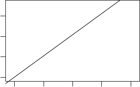
8.7 Checking the Model Assumptions 311
The plot of the partial residual (Fig. 8.5, bottom centre and right panels)
suggest Girth and Height are included on the appropriate scale:
> termplot(cherry.m1, partial.resid=TRUE, las=1)
The line shown on each termplot() represents is the ideal relationship, so
in both cases the plots suggest the model is adequate.
8.7.4 Plots to Check the Random Component
The choice of random component for a glm is usually based on an under-
standing of the data type: proportions of cases are modelled using binomial
glms, and counts by a Poisson glm, for example. However, Q–Q plots may
be used to determine if the choice of distribution is appropriate [5]. Quantile
residuals are used for these plots, since quantile residuals have an exact nor-
mal distribution (apart from sampling variability in estimating μ and φ)if
the correct edm has been chosen.
Example 8.10. Consider the model cherry.m1 (Sect. 8.3) fitted to the cherry
tree data (Example 3.14; data set: trees). A Q–Q plot of the quantile resid-
uals (Fig. 8.6) shows that using a gamma glm seems reasonable.
> qr.cherry <- qresid( cherry.m1 )
> qqnorm( qr.cherry, las=1 ); qqline( qr.cherry)
l
l
l
l
l
l
l
l
l
l
l
l
l
l
l
l
l
l
l
l
l
l
l
l
l
l
l
l
l
l
l
−2 −1 0 1 2
−2
−1
0
1
Normal Q−Q Plot
Theoretical Quantiles
Sample Quantiles
Fig. 8.6 The Q–Q plot of quantile residuals for Model cherry.m1 fitted to the cherry
tree data (Example 8.10)

312 8 Generalized Linear Models: Diagnostics
8.8 Outliers and Influential Observations
8.8.1 Introduction
As for linear regression models, outliers are observations inconsistent with the
rest of the data, and influential observations are outliers that substantially
change the fitted model when removed from the data set. The tools used
to identify outliers (Sect. 3.6.2) and influential observations (Sect. 3.6.3)in
linear regression models are also used for glms, using results from the final
step of the irls algorithm (Sect. 6.3), as discussed next.
8.8.2 Outliers and Studentized Residuals
For glms, as with linear regression models, outliers are identified as obser-
vations with unusually large residuals (positive or negative); the Q–Q plot
is often convenient for doing this. Standardized deviance residuals are com-
monly used, though the use of quantile residuals are strongly encouraged for
discrete data.
As for linear regression, Studentizing the residuals may also be useful
(Sect. 3.6.2). For glms, computing Studentized deviance residuals requires
refitting the original model n further times, when each observation is omit-
ted one at a time. For each model without Observation i, the reduction in the
deviance is computed. Fitting n + 1 models is necessary to do this, which is
computationally expensive, and is avoided by approximating the Studentized
residuals [18]byusing
r
i
= sign(y
i
− ˆμ
i
)
+
1
φ
r
2
D,i
+
h
i
1 − h
i
r
2
P,i
.
If φ is unknown, estimate φ using
¯
φ
(i)
=
D(y, ˆμ) − r
2
D,i
/(1 − h
i
)
n − p
− 1
,
which approximates the mean deviance estimate of φ in the model without
Observation i (written
¯
φ
(i)
). The approximate Studentized deviance residuals
can be found in r using rstudent(), as used for linear regression models.
Example 8.11. Consider the cherry tree data and the model cherry.m1 fitted
in Sect. 8.3 (data set: trees). Compute the raw quantile residuals, raw dev-
iance residuals, standardized deviance residuals, and Studentized residuals:

8.8 Outliers and Influential Observations 313
> library( statmod ) # To compute quantile residuals
> rs <- cbind( rD=resid(cherry.m1), "r'D"=rstandard(cherry.m1),
"r''"=rstudent(cherry.m1), rQ=qresid(cherry.m1))
> head(rs)
rD r'D r'' rQ
1 0.01922903 0.2603676 0.2537382 0.2665369
2 0.03298537 0.4508579 0.4408129 0.4380951
3 0.01295335 0.1803663 0.1756442 0.1882715
4 -0.01321397 -0.1698994 -0.1652566 -0.1380666
5 -0.04709620 -0.6267146 -0.6125166 -0.5606192
6 -0.04640051 -0.6285250 -0.6140386 -0.5519432
> apply( abs(rs), 2, max) # The maximum absolute for each residual
rD r'D r'' rQ
0.166763 2.197761 2.329122 2.053011
Since φ is small in this case, the saddlepoint approximation is suitable
(Sect. 5.4.4), and the quantile, standardized and Studentized residuals are
very similar. No large residuals exist.
8.8.3 Influential Observations
Influential observations are outliers with high leverage. The measures of in-
fluence used for linear regression models, such as Cook’s distance D, dffits,
dfbetas and the covariance ratio, are approximated for glms by using re-
sults from the final iteration of the irls algorithm (Sect. 6.7).
An approximation to Cook’s distance for glmsis
D ≈
r
P
1 − h
2
h
φp
=
(r
P
)
2
p
h
1 − h
(8.5)
as computed by the function cooks.distance() in r, where the Pearson
estimator
¯
φ of φ is used if it is unknown. Thus, Cook’s distance is a combina-
tion of the size of the residual (measured by r
P
) and the leverage (measured
by a monotonic function of h). Applying (8.5) for a linear regression model
produces the same formula for Cook’s distance given in (3.6)(p.110).
dfbetas, dffits, and the covariance ratio cr are computed using the
same formulae as those used in linear regression (Sect. 3.6.3,p.110), using
the deviance residuals and using
¯
φ
(i)
in place of s
2
(i)
. As for linear regres-
sion models, these statistics can be computed in r using dffits() (for df-
fits), dfbetas() (for dfbetas), and covratio() (for cr). The function
influence.measures() returns dfbetas, dffits, cr, D, and the leverages
h, flagging which are deemed influential (or high leverage in the case of h)
according to the criteria in Sect. 3.6.3.

314 8 Generalized Linear Models: Diagnostics
Example 8.12. For the model cherry.m1 fitted to the cherry tree data
(Sect. 8.3; data set: trees), influential observations are identified using
influence.measures():
> im <- influence.measures(cherry.m1); names(im)
[1] "infmat" "is.inf" "call"
> im$infmat <- round(im$infmat, 3 ); head( im$infmat )
dfb.1_ dfb.l(G) dfb.l(H) dffit cov.r cook.d hat
1 0.015 -0.083 0.005 0.107 1.305 0.004 0.151
2 0.120 -0.082 -0.090 0.197 1.311 0.014 0.167
3 0.065 -0.021 -0.054 0.087 1.385 0.003 0.198
4 -0.011 0.021 0.004 -0.041 1.181 0.001 0.059
5 0.145 0.171 -0.170 -0.228 1.218 0.018 0.121
6 0.186 0.191 -0.212 -0.261 1.261 0.023 0.152
> colSums( im$is.inf )
dfb.1_ dfb.l(G) dfb.l(H) dffit cov.r cook.d hat
0000300
Three observations are identified as influential, but only by cr. Since none
of the other measures identify these observations as influential, we should
not be too concerned. Sometimes, plots of the influence statistics are useful
(Fig. 8.7):
> cherry.cd <- cooks.distance( cherry.m1)
> plot( cherry.cd, type="h", ylab="Cook's distance", las=1)
> plot( dffits(cherry.m1), type="h", las=1, ylab="DFFITS")
> infl <- which.max(cherry.cd) # The Observation number of largest D
> infl # Which observation?
18
18
> cherry.cd[infl] # The value of D for that observation
18
0.2067211
0 5 10 20 30
0.00
0.05
0.10
0.15
0.20
Index
Cook's distance
0 5 10 20 30
−0.5
0.0
0.5
Index
DFFITS
Fig. 8.7 Identifying influential observations for model cherry.m1 fitted to the cherry
tree data. Left panel: Cook’s distance; right panel: dffits (Example 8.12)
8.9 Remedies: Fixing Identified Problems 315
The value of Cook’s distance for Observation 18 is much larger than any
others, but the observation is not identified as significantly influential. To
demonstrate, we fit the model without Observation 18, then compare the
estimated coefficients:
> cherry.infl <- update(cherry.m1, subset=(-infl) )
> coef(cherry.m1)
(Intercept) log(Girth) log(Height)
-6.691109 1.980412 1.132878
> coef(cherry.infl)
(Intercept) log(Girth) log(Height)
-7.209148 1.957366 1.267528
(The negative sign in subset=(-infl) omits Observation infl from the
data set for this fit only.) The changes are not substantial, apart perhaps
from the intercept. Contrast to the changes in the coefficients when another
observation with a smaller value of D is omitted:
> cherry.omit1 <- update(cherry.m1, subset=(-1) ) # Omit Obs. 1
> coef(cherry.m1)
(Intercept) log(Girth) log(Height)
-6.691109 1.980412 1.132878
> coef(cherry.omit1)
(Intercept) log(Girth) log(Height)
-6.703461 1.986711 1.131840
The coefficients are very similar to those from model cherry.m1 when Ob-
servation 1 is omitted: Observation 1 is clearly not influential.
8.9 Remedies: Fixing Identified Problems
The techniques of Sects. 8.7 and 8.8 identify weaknesses in the fitted model.
This section discusses possible remedies for these weaknesses. The following
strategy can be adopted:
• If the responses are not independent (Sect. 8.7.2), use other methods,
such as generalized estimating equations [7], generalized linear mixed
models [2, 11] or spatial glms[4, 6]. These are beyond the scope of this
book.
• Ensure the correct edm is used (Sect. 8.7.3); that is, ensure the random
component is adequate. For glms, the response data usually suggest the
edm:
– Proportions of totals may be modelled using a binomial edm
(Chap. 9).
– Count data may be modelled using a Poisson or negative binomial
edm (Chap. 10).
316 8 Generalized Linear Models: Diagnostics
– Positive continuous data may be modelled using a gamma or inverse
Gaussian edm (Chap. 11). In some cases, a Tweedie edm may be
necessary (Sect. 12.2.3).
– Positive continuous data with exact zeros may be modelled using a
Tweedie edm (Sect. 12.2.4).
Occasionally, a mean–variance relationship may be suggested that does
notcorrespondtoanedm. In these cases, quasi-likelihood may be used
(Sect. 8.10), or a different model may be necessary.
• Ensure the systematic component is correct (Sect. 8.7.3):
– The link function may need to change. Changing the link function
may be undesirable, because this changes the relationship between y
and every explanatory variable, and because only a small number of
link functions are useful for interpretability.
– Important explanatory variables may be missing.
– The covariates may need to be transformed. Partial residual plots
may be used to determine if the covariates are included on the correct
scale (and can be produced using termplot()). Simple transforma-
tions, polynomials in covariates (Sect. 3.10) or data-driven systematic
components based on regression splines (Sect. 3.12) may be necessary
in the model. r functions such as poly(), bs() and ns() are used
for glms in the same way as for linear regression models.
Outliers and influential observations also may be remedied by making struc-
tural changes to the model. Sometimes, other strategies are needed to accom-
modate outliers and influential observations, including (under appropriate
circumstances) omitting these observations; see Sect. 3.13.
Example 8.13. A suitable model for the cherry tree data was found in Sect. 8.3
(data set: trees). However, as an example we now consider residual plots
from fitting a naive gamma glm using the default (reciprocal) link function
(Fig. 8.8):
> m.naive <- glm( Volume ~ Girth + Height, data=trees, family=Gamma)
> scatter.smooth( rstandard(m.naive) ~ log(fitted(m.naive)), las=1,
xlab="Fitted values", ylab="Standardized residuals")
> scatter.smooth( rstandard(m.naive) ~ trees$Girth, las=1,
xlab="Girth", ylab="Standardized residuals")
> scatter.smooth( rstandard(m.naive) ~ trees$Height, las=1,
xlab="Height", ylab="Standardized residuals")
> eta <- m.naive$linear.predictor
> z <- resid(m.naive, type="working") + eta
> plot( z ~ eta, las=1,
xlab="Linear predictor, eta", ylab="Working responses, z")
> abline(0, 1, col="grey")
> termplot(m.naive, partial.resid=TRUE, las=1)
(The constant-information scale (Table 8.1) is the logarithmic scale for the
gamma distribution, as used in the top left panel.) The plots of r
D
against

8.9 Remedies: Fixing Identified Problems 317
l
l
l
l
l
l
l
l
l
l
l
l
l
l
l
l
l
l
l
l
l
l
l
l
l
l
ll
l
l
l
3.0 3.5 4.0 4.5
−4
−3
−2
−1
0
1
Fitted values
Standardized residuals
l
l
l
l
l
l
l
l
l
l
l
l
l
l
l
l
l
l
l
l
l
l
l
l
l
l
ll
l
l
l
8121620
−4
−3
−2
−1
0
1
Girth
Standardized residuals
l
l
l
l
l
l
l
l
l
l
l
l
l
l
l
l
l
l
l
l
l
l
l
l
l
l
ll
l
l
l
65 70 75 80 85
−4
−3
−2
−1
0
1
Height
Standardized residuals
l
l
l
l
l
l
l
l
l
l
l
l
l
l
l
l
l
l
l
l
l
l
l
l
l
l
l
l
l
l
l
0.01 0.03 0.05
0.02
0.04
0.06
0.08
Linear predictor, eta
Working responses, z
8121620
−0.03
−0.02
−0.01
0.00
0.01
0.02
0.03
0.04
Girth
Partial for Girth
l
l
l
l
l
l
l
l
l
l
l
l
l
l
l
l
l
l
l
l
l
l
l
l
l
l
l
l
l
l
l
65 70 75 80 85
−0.03
−0.02
−0.01
0.00
0.01
0.02
0.03
0.04
Height
Partial for Height
l
l
l
l
l
l
l
l
l
l
l
l
l
l
l
l
l
l
l
l
l
l
l
l
l
l
l
l
l
l
l
Fig. 8.8 Diagnostic plots for Model m.naive fitted to the cherry tree data. Top left
panel: r
D
against log ˆμ
i
; top centre panel: r
D
against Girth; top right panel: r
D
against
Height; bottom left panel: z against ˆη; bottom centre panel: the partial residual plot for
girth; bottom right panel: the partial residual plot for height (Example 8.13)
log ˆμ (Fig. 8.8, top left panel) and r
D
against the covariates (top centre and
top right panels) show an inadequate systematic component as shown by the
trends and patterns. The plot of z
i
against ˆη
i
(bottom left panel) suggests an
incorrect link function. The partial residual plots (bottom centre and bottom
right panels) suggest the covariates are included in the model incorrectly.
In response to these diagnostic plots, consider the same model but with the
more usual logarithmic link function (Fig. 8.9):
> m.better <- update(m.naive, family=Gamma(link="log"))
> scatter.smooth( rstandard(m.better) ~ log(fitted(m.better)), las=1,
xlab="log(Fitted values)", ylab="Standardized residuals")
> scatter.smooth( rstandard(m.better) ~ trees$Girth, las=1,
xlab="Girth", ylab="Standardized residuals")
> scatter.smooth( rstandard(m.better) ~ trees$Height, las=1,
xlab="Height", ylab="Standardized residuals")
> eta <- m.better$linear.predictor
> z <- resid(m.better, type="working") + eta
> plot( z ~ eta, las=1, las=1,
xlab="Linear predictor, eta", ylab="Working residuals, z")
> abline(0, 1, col="grey")
> termplot(m.better, partial.resid=TRUE, las=1)
The partial residual plots are much improved (Fig. 8.9, bottom centre and
bottom right panels), and the plot of z
i
against ˆη (bottom left panel) suggests

318 8 Generalized Linear Models: Diagnostics
l
l
l
l
l
l
l
l
l
l
l
l
l
l
l
l
l
l
l
l
l
l
l
l
l
l
l
l
l
l
l
2.5 3.0 3.5 4.0 4.5
−2
−1
0
1
log(Fitted values)
Standardized residuals
l
l
l
l
l
l
l
l
l
l
l
l
l
l
l
l
l
l
l
l
l
l
l
l
l
l
l
l
l
l
l
8121620
−2
−1
0
1
Girth
Standardized residuals
l
l
l
l
l
l
l
l
l
l
l
l
l
l
l
l
l
l
l
l
l
l
l
l
l
l
l
l
l
l
l
65 70 75 80 85
−2
−1
0
1
Height
Standardized residuals
l
l
l
l
l
l
l
l
l
l
l
l
l
l
l
l
l
l
l
l
l
l
l
l
l
l
l
l
l
l
l
2.5 3.0 3.5 4.0 4.5
2.5
3.0
3.5
4.0
Linear predictor, eta
Working residuals, z
8121620
−0.5
0.0
0.5
1.0
Girth
Partial for Girth
l
l
l
l
l
l
l
l
l
l
l
l
l
l
l
l
l
l
l
l
l
l
l
l
l
l
l
l
l
l
l
65 70 75 80 85
−0.5
0.0
0.5
1.0
Height
Partial for Height
l
l
l
l
l
l
l
l
l
l
l
l
l
l
l
l
l
l
l
l
l
l
l
l
l
l
l
l
l
l
l
Fig. 8.9 Diagnostic plots for Model m.better fitted to the cherry tree data. Top left
panel: r
D
against log ˆμ
i
; top centre panel: r
D
against Girth; top right panel: r
D
against
Height; bottom left panel: z against ˆη; bottom centre panel: the partial residual plot for
girth; bottom right panel: the partial residual plot for height (Example 8.13)
the correct link function is used. However, the plots of r
D
against log ˆμ (top
left panel) and r
D
against the covariates (top centre and top right panels)
still suggest a structural problem with the model.
In response to these diagnostic plots, model cherry.m1 could be adopted.
The residual plots from model cherry.m1 then show an adequate model
(Fig. 8.5,p.310). In any case, cherry.m1 has sound theoretical grounds, and
should be preferred anyway.
8.10 Quasi-Likelihood and Extended Quasi-Likelihood
In rare cases, sometimes the mean–variance relationship for a data set sug-
gests a distribution that is not an edm. However, the theory developed for
glms is all based on distributions in the edm family. However, note that for
edms, the log-probability function has the neat derivative (Sect. 6.2)
∂ log P(μ, φ; y)
∂μ
=
y −μ
φV (μ)
. (8.6)

8.10 Quasi-Likelihood and Extended Quasi-Likelihood 319
This relationship is used in fitting glms to find the estimates
ˆ
β
j
(Sect. 6.2);
the estimates of β
j
and the standard errors se(
ˆ
β
j
) are consistent given only
the mean and variance information.
Motivated by these results, consider a situation where only the form of the
mean and the variance are known, but no distribution is specified. Since no
distribution is specified, no log-likelihood exists. However, analogous to (8.6),
some quasi-probability function
¯
P exists which satisfies
∂ log
¯
P(y; μ, φ)
∂μ
=
y −μ
φV (μ)
, (8.7)
when only the variance function V (·) is known. On integrating,
log
¯
P(y; μ, φ)=
&
μ
y −u
φV (u)
du.
Suppose we have a series of observations y
i
, for which we assume E[y
i
]=
μ
i
,andvar[y
i
]=φV (μ
i
)/w
i
. Suppose a link-linear predictor for μ
i
in terms
of regression coefficients β
j
,asforaglm. Then the quasi-likelihood function
(more correctly, the quasi-log-likelihood) is defined by
Q(y; μ)=
n
i=1
log
¯
P(y
i
; μ
i
,φ/w
i
).
The quasi-likelihood Q behaves like a log-likelihood function, but does not
correspond to any probability function. As a result, the aic and related statis-
tics (Sect. 7.8) are not defined for quasi-models. In addition, quantile residu-
als (Sect. 8.3.4) are not defined for quasi-likelihood models since the quantile
residuals require the cdf to be defined.
The unit deviance can be defined for quasi-likelihoods. First, notice that
the unit deviance in (5.12) can be written as
d(y, μ)=2{t(y, y) − t(y, μ)}
=2
φ
w
{log P(y; y, φ/w) − log P(y; μ, φ/w)}.
Using the quasi-likelihood in place of the log-likelihood,
d(y, μ)=2
φ
w
"
log
¯
P(y; y, φ/w) − log
¯
P(y; μ, φ/w)
#
=2×
φ
w
&
y
μ
y −u
φV (u)/w
du
=2
&
y
μ
y −u
V (u)
du. (8.8)

320 8 Generalized Linear Models: Diagnostics
In this definition, the unit deviance depends only on the mean and variance.
The total deviance is the (weighted) sum of the unit deviances as usual:
D(y,μ)=
n
i=1
w
i
d(y
i
,μ
i
).
If there exists a genuine edm for which V (μ) is the variance function,
then the unit deviance and all other quasi-likelihood calculations derived
from V (μ) reduce to the usual likelihood calculations for that edm.Thishas
the interesting implication that estimation and inference for glms depends
only on the mean μ and the variance function V (μ). Since quasi-likelihood
estimation is consistent, it follows that estimation for glms is robust against
mis-specification of the probability distribution, because consistency of the
estimates and tests is guaranteed as long as the first and second moment
assumptions (means and variances) are correct.
Quasi-likelihood gives us a way to conduct inference when there is no edm
for a given mean–variance relationship. To specify a quasi-type model struc-
ture, write quasi-glm(V (μ); Link function), where V (μ) is the identifying
variance function.
The most commonly-used quasi-models are for overdispersed Poisson-like
or overdispersed binomial-like counts. These models vary the usual variance
functions in some way, often by assuming a value for the dispersion φ greater
than one, something which is not possible with the family of edms.
We discuss models for overdispersed Poisson-like counts, called quasi-
Poisson models, at some length in Sect. 10.5.3. Quasi-Poisson models are
specified in r using glm() with family=quasipoisson(). We discuss models
for overdispersed binomial-like counts, called quasi-binomial models, at some
length in Sect. 9.8. Quasi-binomial models are specified in r using glm()
with family=quasibinomial(). Other quasi-models are specified in r using
family=quasi(). For more details, see Sect. 8.13.
Inference for these quasi-models uses the same functions as for glms:
summary() shows the results of the Wald tests, and glm.scoretest() in
package statmod performs a score test. anova() performs the equivalent of
likelihood ratio tests for comparing nested models by comparing the quasi-
likelihood, which essentially compares changes in deviance. Analysis of dev-
iance tests are based on the F-tests since φ is estimated for the quasi-models.
Example 8.14. For a Poisson distribution, var[
y]=μ so that V (μ)=μ.How-
ever, in practice, often the variation in the data exceeds μ. This is called
overdispersion (Sect. 10.5). One solution is to propose the variance structure
var[y]=φμ, but this variance structure does not correspond to any discrete
edm. Using quasi-likelihood,
log
¯
P(y; μ, φ)=
&
μ
y −u
φu
du =
y log μ − μ
φ
.

8.11 Collinearity 321
The same algorithms for fitting glms can be used to fit the model based on
this quasi-likelihood. The unit deviance is
d(y, μ)=2
&
y
μ
y −u
u
du =2
y log
y
μ
− (y − μ)
,
identical to the unit deviance for the Poisson distribution (Table 5.1,p.221).
In defining the quasi-likelihood, we considered the derivative of log
¯
P with
respect to μ but not φ. Hence the quasi-probability function is defined only
up to terms not including μ. To deduce a complete quasi-probability function,
the saddlepoint approximation can be used. This gives
log
˜
P(y; μ, φ)=−
1
2
log{2πφV (y)}−
d(y, μ)
2φ
,
which we call the extended quasi-log-probability function. Then
Q
+
(y; μ, φ/w)=
n
i=1
log
˜
P(y
i
; μ
i
,φ/w
i
)
defines the extended quasi-likelihood. Solving dQ
+
(y; μ, φ/w)/dμ =0shows
that the solutions regarding μ are the same as for the quasi-likelihood and
hence the log-likelihood. However, the extended quasi-likelihood has the ad-
vantage that solving dQ
+
(y; μ, φ/w)/dφ = 0 produces the mean deviance
estimate of φ.
The key use of extended quasi-likelihood is to facilitate the estimation of
extended models which contains unknown parameters in the variance function
V (), or which model some structure for the dispersion φ in terms of covariates.
8.11 Collinearity
As in linear regression (Sect. 3.14), collinearity occurs when at least some of
the covariates are highly correlated with each other, implying they measure
almost the same information.
As discussed in Sect. 3.14, collinearity causes no problems in prediction,
but the parameter estimates
ˆ
β
j
are hard to estimate with precision. Several
equations may be found from which to compute the predictions, all of which
may be effective but which produce different interpretations.
322 8 Generalized Linear Models: Diagnostics
Collinearity is most easily identified by examining the correlations between
the covariates. Any correlations greater than some (arbitrary) value, perhaps
0.7, are of concern. Other methods also exist for identifying collinearity. The
same remedies apply as for linear regression (Sect. 3.14):
• Omitting some explanatory variables from the analysis.
• Combine explanatory variables in the model provided the combination
makes sense.
• Collect more data, if there are observations that can be made that better
distinguish the correlated covariates.
• Use special methods, such as ridge regression [17, §11.2], which are beyond
the scope of this book.
Example 8.15. For the cherry tree data (Example 3.14; data set: trees), the
two explanatory variables are correlated:
> cor( trees$Girth, trees$Height)
[1] 0.5192801
> cor( log(trees$Girth), log(trees$Height) )
[1] 0.5301949
Although correlated (that is, taller trees tend to have larger girths), collinear-
ity is not severe enough to be a concern.
8.12 Case Study
The noisy miner data [9] have been used frequently in this book (Example 1.5;
nminer). The glm fitted to model the number of noisy miners Minerab from
the number of eucalypt trees Eucs is:
> library(GLMsData); data(nminer)
> nm.m1 <- glm( Minerab ~ Eucs, data=nminer, family=poisson)
> printCoefmat(coef(summary(nm.m1)))
Estimate Std. Error z value Pr(>|z|)
(Intercept) -0.876211 0.282793 -3.0984 0.001946 **
Eucs 0.113981 0.012431 9.1691 < 2.2e-16 ***
---
Signif. codes: 0 '***' 0.001 '**' 0.01 '*' 0.05 '.' 0.1''1
The diagnostic plots (Fig. 8.10) are informative:
> library(statmod) # To find randomized quantile residuals
> qr <- qresid( nm.m1 )
> qqnorm(qr, las=1); qqline(qr)
> plot( qr ~ sqrt(fitted(nm.m1)), las=1 )
> plot( cooks.distance(nm.m1), type="h", las=1 )
> plot( hatvalues(nm.m1), type="h", las=1 )

8.12 Case Study 323
−2 −1 0 1 2
−3
−2
−1
0
1
2
3
Normal Q−Q Plot
Theoretical Quantiles
Sample Quantiles
l
l
l
l
l
l
l
l
l
l
l
l
l
l
l
l
l
l
l
l
l
l
l
l
l
l
l
l
l
l
High leverage
Large residual
Influential
1.0 1.5 2.0 2.5 3.0 3.5 4.0
−3
−2
−1
0
1
2
3
Quantile residuals vs fitted
values (on const. inf. scale)
μ
^
Quantile residuals
l
l
l
l
l
l
l
l
l
l
l
l
l
l
l
l
l
l
l
l
l
l
l
l
l
l
l
l
l
0 5 10 15 20 25 30
0.0
0.2
0.4
0.6
0.8
Cook's distance
Index
D
i
l
Threshold
0 5 10 15 20 25 30
0.1
0.2
0.3
0.4
0.5
Hat values
Index
h
i
l
Fig. 8.10 Diagnostic plots for the glm fitted to the noisy miner data. Top left: Q–Q
plot of quantile residuals; top right: quantile residuals against
√
ˆμ (using the constant-
information scale for the Poisson distribution); bottom left: Cook’s distance, with the
threshold for significance shown; bottom right: the leverages (Sect. 8.12)
We now locate the observations with the largest leverage, the largest absolute
quantile residual, and the most influential observation:
> maxhat <- which.max( hatvalues(nm.m1) ) # Largest leverage
> maxqr <- which.max( abs(qr) ) # Largest abs. residual
> maxinfl <- which.max( cooks.distance(nm.m1)) # Most influential
> c( MaxLeverage=maxhat, MaxResid=maxqr, MaxInfluence=maxinfl)
MaxLeverage.11 MaxResid MaxInfluence.17
11 7 17
Only Observation 17 is influential according to r’s criterion (Sect. 3.6.3):
> which(influence.measures(nm.m1)$is.inf[,"cook.d"] )
17
17
In summary, Observation 11 (plotted with a filled square) has high leverage,
but the residual is small and so it is not influential; Observation 7 (plotted
with filled circle) has a large residual, but the leverage is small and so it is not

324 8 Generalized Linear Models: Diagnostics
0 5 10 15 20 25 30 35
0
5
10
15
20
Number of eucalypts
Number of noisy miners
ll
l
l
l
l
l
l
l
l
l
l
l
ll
l
l
lllll lll
l
l
l
l
l
High leverage
Large residual
Influential
0 5 10 15 20 25 30 35
0
5
10
15
20
Number of eucalypts
Number of noisy miners
ll
l
l
l
l
l
l
l
l
l
l
l
ll
l
l
lllll lll
l
l
l
l
Original model
Omitting influential
observation
Fig. 8.11 Plots of the noisy miner data: left: the data plotted showing the location of
three important observations; right: the data plotted with the fitted models, with and
without the influential observation, Observation 17 (Sect. 8.12)
influential; Observation 17 (plotted with a filled triangle) has a reasonably
large residual and leverage, and so it is influential.
Observe the changes in the regression coefficients after omitting Observa-
tion 17:
> nm.m2 <- glm( Minerab ~ Eucs, family=poisson, data=nminer,
subset=(-maxinfl)) # A negative index removes the obs.
> c( "Original model"=coef(nm.m1), "Without Infl"=coef(nm.m2))
Original model.(Intercept) Original model.Eucs
-0.8762114 0.1139813
Without Infl.(Intercept) Without Infl.Eucs
-1.0112791 0.1247156
The two fitted models appear slightly different for transects with larger num-
bers of eucalypts (near Observation 17; Fig. 8.11, right panel):
> plot( Minerab ~ jitter(Eucs), data=nminer,
xlab="Number of eucalypts", ylab="Number of noisy miners")
> newE <- seq( 0, 35, length=100)
> newM1 <- predict( nm.m1, newdata=data.frame(Eucs=newE), type="response")
> newM2 <- predict( nm.m2, newdata=data.frame(Eucs=newE), type="response")
> lines( newM1 ~ newE, lty=1); lines( newM2 ~ newE, lty=2)
These results suggest that the two transects with the largest number of
eucalypts are important for understanding the data. Overdispersion may be
an issue for these data, which we explore in Problem 10.10:
> c( deviance(nm.m1), df.residual(nm.m1) )
[1] 63.31798 29.00000
8.13 Using R for Diagnostic Analysis of GLMs 325
8.13 Using R for Diagnostic Analysis of GLMs
Residuals are computed in r for a fitted glm,sayfit, using:
• Pearson residuals r
P
: resid(fit, type="pearson").
• Deviance residuals r
D
: resid(fit), since deviance residuals are the de-
fault.
• Quantile residuals r
Q
: qresid(fit) after loading package statmod.
• Partial residuals u
j
: resid(fit, type="partial").
• Working residuals e: resid(fit, type="working").
• Response residuals y − ˆμ: resid(fit, type="response").
• Standardized deviance residuals r
D
: rstandard(fit).
• Studentized deviance residuals r
D
: approximated using rstudent(fit).
The longer form residuals(fit) is equivalent to resid(fit).Eachtypeof
residual apart from type="partial" returns n values, one for each obser-
vation. Using type="partial" returns an array with n rows and a column
corresponding to each β
j
(apart from β
0
).
Other useful r commands for diagnostics analysis, used in the same way
as for linear regression models, are: fitted(fit) for producing fitted values;
hatvalues(fit) for producing the leverages; qqnorm() for producing Q–Q
plots of residuals; and qqline() for adding reference lines to Q–Q plots.
Measures of influence are computed for glms using the same r functions
as for linear regression models:
• Cook’s distance D:usecooks.distance(fit).
• dfbetas:usedfbetas(fit).
• dffits:usedffits(fit).
• Covariance ratio cr:usecovratio(fit).
All these measures of influence, together with the leverages h, are returned
using influence.measures(fit). Observations are flagged according to the
criteria explained in Sect. 3.6.3 (p. 110).
Fitted glms can also plot()-ed (Sect. 3.16,p.146). These commands pro-
duce four residual plots by default; see ?plot.lm.
For remedying problems, the function poly() is used to create orthogonal
polynomials of covariates, and bs() and ns() (both in the r package splines)
for using regression splines in the systematic component.
Fit quasi-glmsinr using the glm() function, but using specific family
functions:
• quasibinomial() is used to fit quasi-binomial models. The default link
function is the "logit" link function as for binomial glms. "probit",
"cloglog" (complementary log-log), "cauchit" and "log" links are also
permitted, as for binomial glms (Sect. 9.8).
• quasipoisson() is used to fit quasi-Poisson models. The default link
function is the "log" link function as for Poisson glms. "identity" and
"sqrt" links are also permitted, as for Poisson glms (Sect. 10.5.3).
326 8 Generalized Linear Models: Diagnostics
• quasi() is used to fit quasi-models more generally. Because this function
is very general, any of the link functions provided by r are permitted (but
may not all be sensible): "identity" (the default), "logit", "probit",
"cloglog", "cauchit", "log", "identity", "sqrt" and "1/mu^2" are
all permitted. Additional link functions can be defined using the power()
function; for example, link=power(lambda=1/3) uses a link function of
the form μ
1/3
= η.Usinglambda=0 is equivalent to using the logarithmic
link function.
To fit the quasi-models, the variance structure must also be defined,
using for example, family = quasi(link="log", variance="mu"),
which uses the variance function V (μ)=μ. The possible variance struc-
tures permitted for the variance are:
– "constant", the default, for which V (μ) is constant;
– "mu(1-mu)" for which V (μ)=μ(1 −μ);
– "mu" for which V (μ)=μ;
– "mu^2" for which V (μ)=μ
2
;
– "mu^3" for which V (μ)=μ
3
.
Other variance functions can also be specified by writing appropriate r
functions, but are rarely required and require extra effort and so are not
discussed further.
The aic is not shown in the model summary() for quasi-models, since the aic
is not defined for quasi-models. summary(), anova() and glm.scoretest()
work as usual for quasi-models.
8.14 Summary
Chapter 8 discusses methods for identifying possible violations of assumptions
in glms, and then remedying or ameliorating these problems.
The assumptions for glms are, in order of importance (Sect. 8.2):
• Lack of outliers: The model is appropriate for all observations.
• Link function: The correct link function g() is used.
• Linearity: All important explanatory variables are included, and each
explanatory variable is included in the linear predictor on the correct
scale.
• Variance function: The correct variance function V (μ) is used.
• Dispersion: The dispersion parameter φ is constant.
• Independence: The responses y
i
are independent of each other.
• Distribution: The responses y
i
come from the specified edm.
The main tool for diagnostic analysis is residuals. Pearson, deviance and
quantile residuals can be used for glms (Sect. 8.3). Quantile residuals are
highly recommended for discrete edms. Standardized or Studentized resid-
uals are preferred as they have approximately constant variance (Sect. 8.6).

8.14 Summary 327
For glms, the leverages are the diagonal elements of the hat matrix H =
W
1/2
X(X
T
WX)
−1
X
T
W
1/2
(Sect. 8.4.2).
A strategy for diagnostic analysis of glms is (Sects. 8.7 and 8.9):
• Check for independence of the responses (Sect. 8.7.2). If the residuals
show non-independence, use other methods.
• Plot residuals against ˆμ and residuals against each x
j
(Sect. 8.7.3). If the
variation is not constant, an incorrect edm may have been used.
If a trend exists, the systematic component may need changing: change
the link function, add extra explanatory variables, or transform a covari-
ates.
• To further examine the link function, plot z against ˆη (Sect. 8.7.3).
• To determine if the source of the non-linearity is that covariate x
j
is
included on the incorrect scale, plot u
j
against x
j
(called a component
plus residual plot or a partial residual plot) (Sect. 8.7.3).
• The choice of distribution can be checked using a Q–Q plot of quantile
residuals (Sect. 8.7.4).
Outliers can be identified using Studentized residuals (Sect. 8.8). Outliers
and influential observations also may be remedied by changes made to the
model (Sect. 8.8). Influential observations can be identified using Cook’s dis-
tance, dffits, dfbetas or cr (Sect. 8.8).
Quasi-likelihood may be used when a suitable edm cannot be identified,
but information about the mean and variance is available (Sect. 8.10).
Collinearity occurs when at least some of the covariates are highly corre-
lated with each other, implying they measure almost the same information
(Sect. 8.11).
Problems
Selected solutions begin on p. 539.
8.1. Consider the Poisson distribution.
1. For y = 0, show that the smallest possible value of r
P
is −
√
wˆμ.
2. For y = 0, show that the smallest possible value of r
D
is −
√
2wˆμ.
3. For y = 0, what is the smallest value r
Q
can take? Explain.
4. Comment on the normality of the residuals in light of the above results.
8.2. Show that the Pearson residuals for a gamma edm cannot be less than
r
P
= −1/
√
w, but have no theoretical upper limit. Use these results to com-
ment on the approximate normality of Pearson residuals for gamma edms.
What range of values can be taken by deviance and quantile residuals?

328 8 Generalized Linear Models: Diagnostics
8.3. Consider the binomial distribution.
1. Determine the deviance residuals for the binomial distribution.
2. In the extreme case m = 1, show that r
D
will either take the value
2 log(1 − ˆμ)or−
√
2 log ˆμ.
8.4. Use the r function rpois() to generate 1000 random numbers, say y,
from a Poisson distribution with mean 1. Fit a Poisson glm using the system-
atic component y~1. Then, plot the Q–Q plot of the residuals from this model
using the Pearson, deviance and quantile residuals, and comment on the Q–Q
plots produced using the different types of residuals. (Remember to generate
more than one set of quantile residuals due to the added randomness.)
8.5. Consider the situation where the observations y come from distributions
with known mean μ and known φ. Show that the Pearson residuals have
mean zero and variance φ for any edm.
8.6. The standardized deviance residual r
D,i
is approximately the reduction
in the residual deviance when Observation i is omitted from the data. Demon-
strate this in r using the trees data as follows.
• Fit the model cherry.m1 (Sect. 8.3.1). Compute the residual deviance,
the Pearson estimate of φ, and the standardized deviance residuals from
this model.
• Omit Observation 1 from trees, and refit the model. Call this model
cherry.omit1.
• Compute the difference between the residual deviance for the full model
cherry.m1 and for model cherry.omit1. Show that this differences di-
vided by the Pearson estimate of φ is approximately the standardized
deviance residuals squared.
Repeat the above process for every observation i. At each iteration, call this
model cherry.omiti. Then, compute the difference between the deviance for
the full model cherry.lm and for model cherry.omiti. Show that these dif-
ferences divided by φ are approximately the standardized residuals squared.
8.7. Consider the exponential distribution (4.37) defined for y>0.
1. When μ =3.5andy =1.5, compute the Pearson, deviance and quantile
residuals when the weights are all one.
2. When μ =3.5andy =3.5, compute the Pearson, deviance and quantile
residuals when the weights are all one.
3. Comment on what the above shows.
8.8. Consider a transformation A(y) of a response variable y.
1. Expand A(y)aboutμ using the first two terms of the Taylor series to
show that A(y) − A(μ) ≈ A
(μ)(y −μ).

8.14 Summary 329
2. Using the previous result, compute the variance of both sides to show
that
r
A
=
A(y) − A(μ)
A
(μ)
V (μ)
,
called the Anscombe residual [10, 12], has a variance of φ approximately.
3. For glms, A(t)=
'
V (t)
−1/3
(t)dt, where V (μ) is the variance function.
Hence show that the Anscombe residuals for the Poisson distribution are
r
A
=
3(y
2/3
− μ
2/3
)
2μ
1/6
.
4. Compute the Anscombe residuals for the gamma and inverse Gaussian
distributions.
8.9. Suppose a situation implies a variance function of the form V (μ)=
μ
2
(1 − μ)
2
, where 0 <μ<1 (for example, see [10, §9.2.4]). This variance
function does not correspond to any known edm.
1. Deduce the quasi-likelihood.
2. Deduce the unit deviance.
8.10. A study [16] counted the number of birds from four different species of
seabirds in ten different quadrats in the Anadyr Strait (off the Alaskan coast)
during summer, 1998 (Table 8.2; data set: seabirds). Because the responses
are counts, a Poisson glm may be appropriate.
1. Fit the Poisson glm with a logarithmic link function, using the systematic
component Count ~ Species + factor(Quadrat).
2. Using the guidelines in Sect. 7.5 to determine when the Pearson and dev-
iance residuals are expected to be adequate or poor.
3. Using this model, plot the deviance residuals against the fitted values,
and also against the fitted values transformed to the constant-information
scale. Using the plots, determine if the model is adequate.
4. Using the same model, plot the quantile residuals against the fitted values,
and also against the fitted values transformed to the constant-information
scale. Using the plots, determine if the model is adequate.
5. Comparing the plots based on the deviance and quantile residuals, which
type of residual is easier to interpret?
8.11. Children were asked to build towers as high as they could out of cubical
and cylindrical blocks [8, 14]. The number of blocks used and the time taken
were recorded (data set: blocks). In this problem, only consider the number
of blocks used y and the age of the child x.
In Problem 6.10,aglm was fitted for these data. Perform a diagnostic
analysis, and determine if the model is suitable.

330 REFERENCES
Tabl e 8.2 The number of each species of seabird counted in ten quadrats in the Anadyr
Strait during summer, 1998 (Problem 8.10)
Quadrat
Species12345678910
Murre 0 0 0 1 1 0 0 1 1 3
Crestedauklet000231501 5
Leastauklet120000132 3
Puffin101100311 0
8.12. Nambe Mills, Santa Fe, New Mexico [3, 15], is a tableware manufac-
turer. After casting, items produced by Nambe Mills are shaped, ground,
buffed, and polished. In 1989, as an aid to rationalizing production of its 100
products, the company recorded the total grinding and polishing times and
the diameter of each item (Table 5.3; data set: nambeware).
In Problem 6.11,aglm was fitted to these data. Perform a diagnostic
analysis, and determine if the model is suitable.
8.13. In Problem 3.24 (p. 157), a linear regression model was fitted to artifi-
cial data (data set: triangle), generated so that μ =
x
2
1
+ x
2
2
;thatis,x
1
and x
2
are the lengths of the sides of a right-angled triangle, and E[y]=μ is
the length of the hypotenuse (where some randomness has been added).
1. Based on the true relationships between the variables, write down the
corresponding systematic component for fitting a glm for modelling the
hypotenuse. What link function is necessary?
2. Fit an appropriate glm to the data, using the normal and gamma distri-
butions to model the randomness. Which glm is preferred?
References
[1] Box, G.E.P.: Science and statistics. Journal of the American Statistical
Association 71, 791–799 (1976)
[2] Breslow, N.E., Clayton, D.G.: Approximate inference in generalized lin-
ear mixed models. Journal of the American Statistical Association
88(421), 9–25 (1993)
[3] Data Desk: Data and story library (dasl) (2017). URL http://dasl.
datadesk.com
[4] Diggle, P.J., Tawn, J.A., Moyeed, R.A.: Model-based geostatistics. Ap-
plied Statistics 47(3), 299–350 (1998)
[5] Dunn, P.K., Smyth, G.K.: Randomized quantile residuals. Journal of
Computational and Graphical Statistics 5(3), 236–244 (1996)
REFERENCES 331
[6] Gotway, C.A., Stroup, W.W.: A generalized linear model approach to
spatial data analysis and prediction. Journal of Agricultural, Biological
and Environmental Statistics 2(2), 157–178 (1997)
[7] Hardin, J.W., Hilbe, J.M.: Generalized Estimating Equations. Chapman
and Hall/CRC, Boca Raton (2012)
[8] Johnson, B., Courtney, D.M.: Tower building. Child Development 2(2),
161–162 (1931)
[9] Maron, M.: Threshold effect of eucalypt density on an aggressive avian
competitor. Biological Conservation 136, 100–107 (2007)
[10] McCullagh, P., Nelder, J.A.: Generalized Linear Models, second edn.
Chapman and Hall, London (1989)
[11] McCulloch, C.E.: Generalized linear mixed models. Institute of Mathe-
matical Statistics (2003)
[12] Pierce, D.A., Shafer, D.W.: Residuals in generalized linear models. Jour-
nal of the American Statistical Association 81, 977–986 (1986)
[13] Pregibon, D.: Goodness of link tests for generalized linear models. Ap-
plied Statistics 29(1), 15–24 (1980)
[14] Singer, J.D., Willett, J.B.: Improving the teaching of applied statistics:
Putting the data back into data analysis. The American Statistician
44(3), 223–230 (1990)
[15] Smyth, G.K.: Australasian data and story library (Ozdasl) (2011).
URL http://www.statsci.org/data
[16] Solow, A.R., Smith, W.: Detecting in a heterogenous community sam-
pled by quadrats. Biometrics 47(1), 311–317 (1991)
[17] Weisberg, S.: Applied Linear Regression. John Wiley and Sons, New
York (1985)
[18] Williams, D.A.: Generalized linear models diagnostics using the deviance
and single-case deletions. Applied Statistics 36(2), 181–191 (1987)

Chapter 9
Models for Proportions: Binomial
GLMs
We believe no statistical model is ever final; it is simply a
placeholder until a better model is found.
Singer and Willett [22, p. 105]
9.1 Introduction and Overview
Chapters 5–8 develop the theory of glms in general. This chapter focuses on
one specific glm: the binomial glm. The binomial glm is the most commonly
used of all glms. It is used to model proportions, where the proportions are
obtained as the number of ‘positive’ cases out of a total number of inde-
pendent cases. We first compile important information about the binomial
distribution (Sect. 9.2), then discuss the common link functions used for bi-
nomial glms (Sect. 9.3), and the threshold interpretation of the link function
(Sect. 9.4). We then discuss model interpretation in terms of odds (Sect. 9.5),
and how binomial glms can be used to estimate the median effective dose
ed50 (Sect. 9.6). The issue of overdispersion is then discussed (Sect. 9.8), fol-
lowed by a warning about a potential problem with parameter estimation in
binomial glms (Sect. 9.9). Finally, we explain why goodness-of-fit tests are
not appropriate for binary data (Sect. 9.10).
9.2 Modelling Proportions
The outcome of many studies is a proportion y of a total number m:the
proportion of individuals having a disease; the proportion of voters who vote
in favour of a particular election candidate; the proportion of insects that die
after being exposed to different doses of a poison. For all these examples, a
binomial distribution may be an appropriate response distribution. In each
case, the m individuals in each group are assumed to be independent, and
each individual can be classified into one of two possible outcomes.
The binomial distribution has already been established as an edm
(Example 5.3), and binomial glms used in examples in previous chapters to
© Springer Science+Business Media, LLC, part of Springer Nature 2018
P. K. Dunn, G. K. Smyth, Generalized Linear Models with Examples in R,
Springer Texts in Statistics, https://doi.org/10.1007/978-1-4419-0118-7_9
333

334 9 Models for Proportions: Binomial GLMs
develop the theory of glms. Useful information about the binomial distribu-
tion appears in Table 5.1 (p. 221). The probability function for a binomial
edm is
P(y; μ, m)=
m
my
μ
my
(1 − μ)
m(1−y)
(9.1)
where m is known and φ = 1, and where y =0, 1/m, 2/m,...1, and the
expected proportion is 0 <μ<1. To use the binomial distribution in a glm,
the prior weights w are set to the group totals m. The unit deviance for the
binomial distribution is
d(y, μ)=2
y log
y
μ
+(1− y) log
1 − y
1 − μ
.
When y =0ory = 1, the limit form of the unit deviance (5.14) is used.
The residual deviance is D(y, ˆμ)=
n
i=1
m
i
d(y
i
, ˆμ
i
). By the saddlepoint
approximation, D(y, ˆμ) ∼ χ
2
n−p
for a model with p
parameters in the linear
predictor. The saddlepoint approximation is adequate if min{m
i
y
i
}≥3and
min{m
i
(1 − y
i
)}≥3 (Sect. 7.5).
A binomial glm is denoted glm(binomial; link), and is specified in r using
family=binomial() in the glm() call. Binomial responses may be specified
in the glm() formula in one of three ways:
1. The response can be supplied as the observed proportions y
i
, when the
sample sizes m
i
are supplied as the weights in the call to glm().
2. The response can be given as a two-column array, the columns giving the
numbers of successes and failures respectively in each group of size m
i
.
The prior weights weights do not need to be supplied (r computes the
weights m as the sum of the number of successes and failures for each
row).
3. The response can be given as a factor (when the first factor level corre-
sponds to failures, and all others levels to successes) or as a logicals (ei-
ther TRUE, which is treated as the success, or FALSE). The prior weights
weights do not need to be supplied in this specification (and are set to
one by default). This specification is useful if the data have one row for
each observation (see Example 9.1). In this form, the responses are binary
and the model is a Bernoulli glm (see Example 4.6). While many of the
model statistics are the same (Problem 9.14), there are some limitations
with using this form (Sect. 9.10).
For binomial glms, the use of quantile residuals [5] is strongly recommended
for diagnostic analysis (Sect. 8.3.4.2).
Example 9.1. An experiment running turbines for various lengths of time [19,
20] recorded the proportion of turbine wheels y
i
out of a total of m
i
turbines
developing fissures (narrow cracks) (Table 9.1; Fig. 9.1; data set: turbines).
A suitable model for the data may be a binomial glm.

9.2 Modelling Proportions 335
Tabl e 9. 1 The number of turbine wheels developing fissures and the number of hours
they are run (Example 9.1)
Prop. of No. of Prop. of No. of
Case Hours Turbines fissures fissures Case Hours Turbines fissures fissures
ix
i
m
i
y
i
m
i
y
i
ix
i
m
i
y
i
m
i
y
i
1 400 39 0.0000 0 7 3000 42 0.2143 9
2 1000 53 0.0755 4 8 3400 13 0.4615 6
3 1400 33 0.0606 2 9 3800 34 0.6471 22
4 1800 73 0.0959 7 10 4200 40 0.5250 21
5 2200 30 0.1667 5 11 4600 36 0.5833 21
6 2600 39 0.2308 9
l
l
l
l
l
l
l
l
l
l
l
0 1000 2000 3000 4000 5000
0.0
0.1
0.2
0.3
0.4
0.5
0.6
0.7
Hours of use
Proportion of turbines
with fissures
1
2
3
4
5
6
7
8
9
10
11
1
2
3
4
5
6
7
8
9
10
11
Fig. 9.1 The proportion of turbine wheels developing fissures plotted against the num-
ber of hours of use. Larger plotting symbols indicate proportions based on larger sample
sizes. The numbers beside the points refer to the case number (Example 9.1)
For these data, the first and second forms of specifying the response are
appropriate and equivalent:
> library(GLMsData); data(turbines)
> tur.m1 <- glm( Fissures/Turbines ~ Hours, family=binomial,
weights=Turbines, data=turbines)
> tur.m2 <- glm( cbind(Fissures, Turbines-Fissures) ~ Hours,
family=binomial, data=turbines)
> coef(tur.m1); coef(tur.m2)
(Intercept) Hours
-3.9235965551 0.0009992372
(Intercept) Hours
-3.9235965551 0.0009992372
To use the third form of data entry, the data would need to be rearranged
so that each individual turbine was represented in its own line, hence having
n
i=1
m
i
= 432 rows.

336 9 Models for Proportions: Binomial GLMs
9.3 Link Functions
Specific link functions are required for binomial glms to ensure that 0 <
μ<1. Numerous suitable choices are available. Three link functions are
commonly used with the binomial distribution:
1. The logit (or logistic) link function, which is the canonical link function
for the binomial distribution and the default link function in r:
η = log
μ
1 − μ
= logit(μ). (9.2)
(r uses natural logarithms.) This link function is specified in r using
link="logit". A binomial glm with a logit link function is often called
a logistic regression model.
2. The probit link function: η = Φ
−1
(μ) = probit(μ), where Φ(·)isthe
cdf for the normal distribution. This link function is specified in r as
link="probit".
3. The complementary log-log link function: η = log{−log(1−μ)}. This link
function is specified in r as link="cloglog".
In practice, the logit and probit link functions are very similar (Fig. 9.2). In
addition, both are symmetric about μ =0.5, whereas the complementary
log-log link function is not.
Two other less common link functions permitted in r for binomial glms
are the "cauchit" and "log" links. The "cauchit" link function is based
on the Cauchy distribution (see Sect. 9.4), but is rarely used in practice. The
−4 −2 0 2 4
0.0
0.2
0.4
0.6
0.8
1.0
The linear predictor η
The expected proportion μ
Logistic
Probit
Comp. log−log
Fig. 9.2 Common link functions used with the binomial distribution: the logit, probit,
and complementary log-log link functions (Sect. 9.3)

9.3 Link Functions 337
0246810
0.0
0.2
0.4
0.6
0.8
1.0
x
The expected proportion, μ
η=−5 + x
η=−5 + 2x
0246810
0.0
0.2
0.4
0.6
0.8
1.0
x
The expected proportion, μ
η=5 − x
η=5 − 2x
Fig. 9.3 The relationships between x and the predicted proportions μ for various linear
predictors η using the logit link function, where logit(μ)=η (Sect. 9.3)
"log" link function is sometimes used for modelling risk ratios or relative
risks. It is an approximation to the logit link when μ is small [16].
To understand the relationship between the explanatory variables and μ,
consider the case of one explanatory variable where η = β
0
+ β
1
x. Figure 9.3
shows the corresponding relationships between x and μ using the logit link
function.
Example 9.2. For the turbine data (data set: turbines), we can fit binomial
glms using the three common link functions, using the hours run-time as the
explanatory variable:
> tr.logit <- glm( Fissures/Turbines ~ Hours, data=turbines,
family=binomial, weights=Turbines)
> tr.probit <- update( tr.logit, family=binomial(link="probit") )
> tr.cll <- update( tr.logit, family=binomial(link="cloglog") )
> tr.array <- rbind( coef(tr.logit), coef(tr.probit), coef(tr.cll))
> tr.array <- cbind( tr.array, c(deviance(tr.logit),
deviance(tr.probit), deviance(tr.cll)) )
> colnames(tr.array) <- c("Intercept", "Hours","Residual dev.")
> rownames(tr.array) <- c("Logit","Probit","Comp log-log")
> tr.array
Intercept Hours Residual dev.
Logit -3.923597 0.0009992372 10.331466
Probit -2.275807 0.0005783211 9.814837
Comp log-log -3.603280 0.0008104936 12.227914
The residual deviances are similar for the logit and probit glms, and slightly
larger for the complementary log-log link function. The coefficients from the
three models are reasonably different. However, the models themselves are
very similar, as we can see by plotting the models. To do so, first set up a
vector of values for the run-time:
> newHrs <- seq( 0, 5000, length=100)

338 9 Models for Proportions: Binomial GLMs
l
l
l
l
l
l
l
l
l
l
l
l
0 1000 2000 3000 4000 5000
0.0
0.1
0.2
0.3
0.4
0.5
0.6
0.7
Hours run
Proportion with fissures
Logit
Probit
Comp. log−log
Fig. 9.4 The turbines data, showing the fitted binomial glms, using logistic, probit
and complementary log-log link functions (Example 9.2)
Now, make predictions from these values using each model:
> newdf <- data.frame(Hours=newHrs)
> newP.logit <- predict( tr.logit, newdata=newdf, type="response")
> newP.probit <- predict( tr.probit, newdata=newdf, type="response")
> newP.cll <- predict( tr.cll, newdata=newdf, type="response")
The type of prediction is set as "response" because, by default, predict()
returns the predictions on the linear predictor scale (that is, ˆη is returned
rather than ˆμ). Now, plot these predictions using lines(), then add a legend
(Fig. 9.4):
> plot( Fissures/Turbines ~ Hours, data=turbines, pch=19, las=1,
xlim=c(0, 5000), ylim=c(0, 0.7),
xlab="Hours run", ylab="Proportion with fissures")
> lines( newP.logit ~ newHrs, lty=1, lwd=2)
> lines( newP.probit ~ newHrs, lty=2, lwd=2)
> lines( newP.cll ~ newHrs, lty=4, lwd=2)
> legend("topleft", lwd=2, lty=c(1, 2, 4),
legend=c("Logit","Probit","Comp. log-log"))
All three models produce similar predictions, which is not unusual.
9.4 Tolerance Distributions and the Probit Link
The link functions can be understood using a threshold interpretation. In
what follows, we show how the threshold interpretation applies for the probit
link function, using the turbines data as the example.
Assume each individual turbine has a different tolerance beyond which
it will develop fissures. As part of the natural variation in turbines, this

9.4 Tolerance Distributions and the Probit Link 339
tolerance varies from turbine to turbine (but is fixed for any one turbine).
Denote this tolerance level as t
i
for turbine i; note that t
i
is a continuous
variable. Assume that t
i
follows a normal distribution with mean tolerance
τ
i
,sothat
t
i
∼ N(τ
i
,σ
2
)
τ
i
= β
0
+ β
1
x
i
,
(9.3)
where x
i
is the number of hours that turbine i is run. In this context, the
normal distribution in (9.3) is called the tolerance distribution.
The variable of interest is whether or not the turbines develop fissures.
Assume that turbines develop fissures if the tolerance level t
i
of turbine i is
less than some fixed tolerance threshold T . In other words, define
y
i
=
1ift
i
≤ T , and the turbine develops fissures
0ift
i
>T, and the turbine does not develop fissures.
Then, the probability that turbine i develops fissures is
μ
i
=Pr(y
i
=1)=Pr(t
i
≤ T )=Φ
T − τ
i
σ
, (9.4)
where Φ(·)isthecdf of the standard normal distribution. We can write
T − τ
i
σ
=
T − β
0
− β
1
x
i
σ
= β
0
+ β
1
x
i
with β
0
=(T − β
0
)/σ and β
1
= −β
1
/σ. Then (9.4) becomes
g(μ
i
)=β
0
+ β
1
x
i
where g() is the probit link function.
Other choices of the tolerance distribution lead to other link functions
by a similar process (Table 9.2). The logit link function emerges as the link
function when the logistic distribution is used as the tolerance distribution
(Problem 9.4). The complementary log-log link function emerges as the link
function when the extreme value (or Gumbel) distribution is used as the
tolerance distribution. The cauchit link function assumes the threshold dis-
tribution is the Cauchy distribution. The logistic and normal tolerance dis-
tributions are both symmetric, and usually give similar results except for
probabilities near zero or one. In contrast, the extreme value distribution is
not symmetric, so the complementary log-log link function often gives some-
what different results than using the logit and probit link functions (Fig. 9.2).
In principle, the cdf for any continuous distribution can be used as a basis
for the link function.

340 9 Models for Proportions: Binomial GLMs
Tabl e 9 . 2 Tolerance distributions leading to link functions for binomial glms(Sect.9.3)
Link function Tolerance distribution Distribution function
Logit Logistic F(y)=exp(y)/ {1+exp(y)}
Probit Normal F(y)=Φ(y)
Complementary log-log Extreme value F(y)=1− exp {−exp(y)}
Cauchit Cauchy F(y)={arctan(y)+0.5}/π
9.5 Odds, Odds Ratios and the Logit Link
Using the logit link function with the binomial distribution produces a useful
interpretation. To understand this interpretation, the concept of odds first
must be understood. If event A has probability μ of occurring, then the odds
of event A occurring is the ratio of the probability that A occurs to the
probability that A does not occur: μ/(1 −μ). For example, if the probability
that a turbine develops fissures is 0.6, the odds that a turbine develops fissures
is 0.6/(1 − 0.6) = 1.5. This means that the probability of observing fissures
is 1.5 times greater than the probability of not observing a fissure (that is,
1.5 × 0.4=0.6). Clearly, using the logit link function in a binomial glm is
equivalent to modelling the logarithm of the odds (or the ‘log-odds’).
The binomial glm using the logit function can be written as
log(odds) = β
0
+ β
1
x
or equivalently odds = exp(β
0
){exp(β
1
)}
x
.
As x increases by one unit, the log-odds increase by linearly by an amount
β
1
. Alternatively, if x increases by one unit, the odds increase by a factor of
exp(β
1
). These interpretations in terms of the odds have intuitive appeal, and
for this reason the logit link function is often preferred for the link function.
Example 9.3. For the turbines data (data set: turbines), the fitted logistic
regression model (Example 9.1) has coefficients:
> coef(tr.logit)
(Intercept) Hours
-3.9235965551 0.0009992372
In this model, increasing Hours by one increases the odds of a turbine de-
veloping fissures by exp(0.0009992) = 1.001. In this case, the interpretation
is more useful if we consider increasing Hours by 1000 h. This increases the
odds of a turbine developing fissures by exp(1000×0.0009992) = 2.716 times.
Using the logistic regression model tr.logit assumes that the relationship
between the run-time and the log-odds is approximately linear (Fig. 9.5):
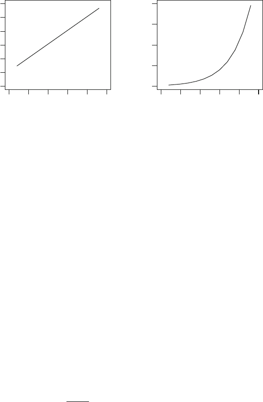
9.5 Odds, Odds Ratios and the Logit Link 341
0 1000 3000 5000
−5
−4
−3
−2
−1
0
1
Run−time (in hours)
Log−odds
l
l
l
l
l
l
l
l
l
l
l
0 1000 3000 5000
0.0
0.5
1.0
1.5
2.0
Run−time (in hours)
Odds
l
l
l
l
l
l
l
l
l
l
l
Fig. 9.5 The log-odds plotted against the run-time (left panel) and the odds plotted
against the run-time (right panel) for the binomial logistic glm fitted to the turbine
data (Example 9.3)
> LogOdds <- predict( tr.logit ); odds <- exp( LogOdds )
> plot( LogOdds ~ turbines$Hours, type="l", las=1,
xlim=c(0, 5000), ylim=c(-5, 1),
ylab="Log-odds", xlab="Run-time (in hours)" )
> my <- turbines$Fissures; m <- turbines$Turbines
> EmpiricalOdds <- (my + 0.5)/(m - my + 0.5) # To avoid log of zeros
> points( log(EmpiricalOdds) ~ turbines$Hours)
>#
> plot( odds ~ turbines$Hours, las=1, xlim=c(0, 5000), ylim=c(0, 2),
type="l", ylab="Odds", xlab="Run-time (in hours)")
> points( EmpiricalOdds ~ turbines$Hours)
Note the use of empirical log-odds, adding 0.5 to both the numerator and
denominator of the odds, so that the log-odds can be computed even when
y =0.
Logistic regression models are often fitted to data sets that include factors
as explanatory variables. In these situations, the concept of the odds ratio is
useful to define. Consider the binomial glm with systematic component
log
μ
1 − μ
= log-odds = β
0
+ β
1
x,
where x is a dummy variable taking the values 0 or 1. From this equation,
we see that the odds of observing a success when x = 0 is exp(β
0
), and the
odds of observing a success when x = 1 is exp(β
0
+ β
1
) = exp(β
0
)exp(β
1
).
The ratio of these two odds is exp(β
1
). This means that the odds of a success
occurring when x = 1 is exp(β
1
) times greater than when x = 0. This ratio is
called the odds ratio, often written or. When a number of factors are fitted
as explanatory variables, each of the corresponding regression parameters β
j
can be interpreted as odds ratios in a similar manner.

342 9 Models for Proportions: Binomial GLMs
Tabl e 9. 3 The germination of two types of seeds for two root extracts. The number of
seeds germinating my from m seeds planted is shown (Table 9.4)
O. aegyptiaco 75 seeds O. aegyptiaco 73 seeds
Bean extracts Cucumber extracts Bean extracts Cucumber extracts
my m my m my m my m
10 39 5 6 8 16 3 12
23 62 53 74 10 30 22 41
23 81 55 72 8 28 15 30
26 51 32 51 23 45 32 51
17 39 46 79 0 4 3 7
10 13
Bean Cucumber
0.0
0.2
0.4
0.6
0.8
1.0
Extract
Germ/Total
OA73 OA75
0.0
0.2
0.4
0.6
0.8
1.0
Seeds
Germ/Total
Fig. 9.6 The germination data: germination proportions plotted against extract type
(left panel) and seed type (right panel) (Example 9.4)
Example 9.4. A study [3] of seed germination used two types of seeds and two
typesofrootstocks(Table9.3; data set: germ). A plot of the data (Fig. 9.6)
shows possible relationships between the proportions of seeds germinating
and both factors:
> data(germ); str(germ)
'data.frame': 21 obs. of 4 variables:
$ Germ : int 10 23 23 26 17 5 53 55 32 46 ...
$ Total : int 39 62 81 51 39 6 74 72 51 79 ...
$ Extract: Factor w/ 2 levels "Bean","Cucumber": 1111122222...
$ Seeds : Factor w/ 2 levels "OA73","OA75": 2222222222...
> plot( Germ/Total ~ Extract, data=germ, las=1, ylim=c(0, 1) )
> plot( Germ/Total ~ Seeds, data=germ, las=1, ylim=c(0, 1) )
The model with both factors as explanatory variables can be fitted:
> gm.m1 <- glm(Germ/Total ~ Seeds + Extract, family=binomial,
data=germ, weights=Total)
> printCoefmat(coef(summary(gm.m1)))

9.6 Median Effective Dose, ED50 343
Estimate Std. Error z value Pr(>|z|)
(Intercept) -0.70048 0.15072 -4.6475 3.359e-06 ***
SeedsOA75 0.27045 0.15471 1.7482 0.08044 .
ExtractCucumber 1.06475 0.14421 7.3831 1.546e-13 ***
---
Signif. codes: 0 '***' 0.001 '**' 0.01 '*' 0.05 '.' 0.1''1
Recall the r output means that the r variable Seeds takes the value one for
OA75 and is zero for OA73. Likewise the r variable Extract takes the value
one for Cucumber and is zero for Bean.
Note that
> exp( coef(gm.m1) )
(Intercept) SeedsOA75 ExtractCucumber
0.4963454 1.3105554 2.9001133
This means that the odds of seed germination occurring using cucumber
extracts is 2.900 times the odds of seed germination occurring using bean
extracts. Similarly, the odds of seed germination occurring using O. aegypti-
aco 75 seeds are 1.311 times the odds of seed germination occurring using O.
aegyptiaco 73 seeds.
These data are explored later also (Example 9.8), where the interaction
term is considered.
9.6 Median Effective Dose, ED50
Binomial glms are commonly used to examine the relationship between the
dose d of a drug or poison and the proportion y of insects (or plants, or
animals) that survive. These models are called dose–response models. Asso-
ciated with these experiments is the concept of the median effective dose,
ed50: the dose of poison affecting 50% of the insects. Different fields use dif-
ferent names for similar concepts, such as median lethal dose ld50 or median
lethal concentration lc50. Here, for simplicity, we use ed50 to refer to any
of these quantities. The ed50 concept can be applied to other contexts also.
By definition, μ =0.5attheed50.
For a binomial glm using a logit link function, η = logit(μ) = 0 when
μ =0.5. Writing the linear predictor as η = β
0
+ β
1
d where d is the dose,
then solving for the dose d shows that ed50 = −
ˆ
β
0
/
ˆ
β
1
. More generally,
the dose effective on any proportion ρ of the population, denoted ed(ρ), is
estimated by
ed(ρ)=
g(ρ) − β
0
β
1
,
where g() refers to the link function used in fitting the model. In Problem 9.2,
formulae are developed for computing ed50 for the probit and complementary
log-log link functions.
344 9 Models for Proportions: Binomial GLMs
The function dose.p() in the r package MASS (which comes with r
distributions) conveniently returns
ed(ρ) and the corresponding estimated
standard error. The first input to dose.p() is the glm() object, and the
second input identifies the two coefficients of importance: the coefficient for
the intercept and for the dose (in that order). By default, these are assumed
to be the first and second coefficients. The third input is ρ; by default ρ =0.5,
and so
ed50 is returned by default.
Example 9.5. Consider the turbine data again (data set: turbines). The ed50
corresponds to the run time for which 50% of turbines would be expected to
experience fissures:
> library(MASS) # MASS comes with R
> ED50s <- cbind("Logit" = dose.p(tr.logit),
"Probit" = dose.p(tr.probit),
"C-log-log" = dose.p(tr.cll))
> ED50s
Logit Probit C-log-log
p = 0.5: 3926.592 3935.197 3993.575
Running the turbines for approximately 3927 h would produce fissures in
about 50% of the turbines (using the logistic link function model). All three
link functions produce similar estimates of ed50, which seems reasonable
based on Fig. 9.4 (p. 338).
9.7 The Complementary Log-Log Link in Assay Analysis
A common problem in biology is to determine the proportion of cells or
organisms of interest amongst a much larger population. For example, does
a sample of tissue contain infective bacteria, and how many? Or what is the
frequency of adult stem cells in a sample of tissue?
Suppose the presence of active particles can be detected by undertaking an
assay. For example, the presence of bacteria might be detected by incubating
the sample on an agar plate, and observing whether a bacterial culture grows.
Or the presence of stem cells might be detected by transplanting cells into a
host animal, and observing whether a new growth occurs. However, the same
response is observed, more or less, regardless of the number of active particles
in the original sample. A single stem cell would result in a new growth. When
a growth is observed, we cannot determine directly whether there was one
stem cell or many to start with.
Dilution assays are an experimental technique to estimate the frequency
of active cells. The idea is to dilute the sample down to the point where some
assays yield a positive result (so at least one active particles is present) and
some yield a negative result (so no active particles are present).
The fundamental property of limiting dilution assays is that each assay
results in a positive or negative result. Write μ
i
for the probability of a
9.7 The Complementary Log-Log Link in Assay Analysis 345
positive result given that the expected number of cells in the culture is d
i
.
If m
i
independent cultures are conducted at dose d
i
, then the number of
positive results follows a binomial distribution.
Write λ for the proportion of active cells in the cell population, so that
the expected number of active cells in the culture is λd
i
. If the cells behave
independently (that is, if there are no community effects amongst the cells),
and if the cell dose is controlled simply by dilution, then the actual number of
cells in each culture will vary according to a Poisson distribution. A culture
will give a negative result only if there are no active cells in the assay. The
Poisson probability formula tells us that this occurs with probability
1 − μ
i
=exp(−λd
i
).
This formula can be linearized by taking logarithms of both sides, as
log(1 − μ
i
)=−λd
i
(9.5)
or, taking logarithms again,
log{−log(1 − μ
i
)} = log λ + log d
i
. (9.6)
This last formula is the famous complementary log-log transformation from
Mather [18].
The proportion of active cells can be estimated by fitting a binomial glm
with a complementary log-log link:
g(μ
i
)=β
0
+ log d
i
(9.7)
where log d
i
is an offset and g() is the complementary log-log link function.
The estimated proportion of active cells is then
ˆ
λ =exp(
ˆ
β
0
).
In principle, a glm could also have be fitted using (9.5) as a link-linear
predictor, in this case with a log-link. However (9.6) is superior, because it
leads to a glm (9.7) without any constraints on the coefficient β
0
.
As usual, a confidence interval is given by
ˆ
β
0
± z
α/2
se(
ˆ
β
0
)
where se(
ˆ
β
0
) is the standard error of the estimate and z
α/2
is the critical
value of the normal distribution, e.g., z =1.96 for a 95% confidence interval.
To get back to the active cell frequency simply exponentiate and invert the
estimate and the confidence interval: 1/
ˆ
λ =exp(−
ˆ
β
0
). Confidence intervals
can be computed for 1/λ, representing the number of cells required on average
to obtain one responding cell.
The dilution assay model assumes that a single active cell is sufficient
to achieve a positive result, so it is sometimes called the single-hit model
(though other assumptions are possible [25]). One way to check this model is

346 9 Models for Proportions: Binomial GLMs
Tabl e 9 .4 The average number of cells in each assay in which cells were transplanted
in host mice, the number of assays at that cell number, and the number of assays giving
a positive outcome, a milk gland outgrowth (Example 9.6)
Number of cells Number of Number of
per assay assays outgrowths
15 38 3
40 6 6
60 17 13
90 8 6
125 12 9
to fit a slightly larger model in which the offset coefficient is not set to one:
g(μ
i
)=β
0
+ β
1
log d
i
.
The correctness of the single-hit model can then be checked [10] by testing
the null hypothesis H
0
: β
1
=1.
Example 9.6. Shackleton et al. [21] demonstrated the existence of adult mam-
mary stem cells. They showed, for the first time, that a complete mammary
milk producing gland could be produced in mice from a single cell. After a
series of steps, they were able to purify a population of cells that was highly
enriched for mammary stem cells, although stem cells were still a minority
of the total.
The data (Table 9.4; data set: mammary) relate to a number of assays in
which cells were transplanted into host mice. A positive outcome here consists
of seeing a milk gland outgrowth, evidence that the sample of cells included
as least one stem cell. The data give the average number of cells in each assay,
the number of assays at that cell number, and the number of assays giving a
positive outcome.
> data(mammary); mammary
N.Cells N.Assays N.Outgrowths
115 38 3
240 6 6
360 17 13
490 8 6
5 125 12 9
> y <- mammary$N.Outgrowths / mammary$N.Assays
> fit <- glm(y~offset(log(N.Cells)), family=binomial(link="cloglog"),
weights=N.Assays, data=mammary)
> coef(summary(fit))
Estimate Std. Error z value Pr(>|z|)
(Intercept) -4.163625 0.1744346 -23.86925 6.391454e-126
> frequency <- 1/exp(coef(fit)); frequency
(Intercept)
64.30418
9.8 Overdispersion 347
The mammary stem cell frequency is estimated to be about 1 in 64 cells. A
95% confidence interval is computed as follows:
> s <- summary(fit)
> Estimate <- s$coef[, "Estimate"]
> SE <- s$coef[, "Std. Error"]
> z <- qnorm(0.05/2, lower.tail=FALSE)
> CI <- c(Lower=Estimate+z*SE, Estimate=Estimate, Upper=Estimate-z*SE)
> CI <- 1/exp(CI); round(CI, digits=1)
Lower Estimate Upper
45.7 64.3 90.5
The frequency of stem cells is between 1/46 and 1/91. There is no evidence
of any deviation from the single-hit model:
> fit1 <- glm(y~log(N.Cells), family=binomial(link="cloglog"),
weights=N.Assays, data=mammary)
> anova(fit, fit1, test="Chisq")
Analysis of Deviance Table
Model 1: y ~ offset(log(N.Cells))
Model 2: y ~ log(N.Cells)
Resid. Df Resid. Dev Df Deviance Pr(>Chi)
1 4 16.852
2 3 16.205 1 0.6468 0.4213
9.8 Overdispersion
For a binomial distribution, var[y]=μ(1 − μ). However, in practice the
amount of variation in the data can exceed μ(1 − μ), even for ostensibly
binomial-like data. This is called overdispersion. Underdispersion also occurs,
but is less common.
Overdispersion has serious consequences for the glm. It means that stan-
dard errors returned by the glm are underestimated, and tests on the ex-
planatory variables will generally appear to be more significant that war-
ranted by the data, leading to overly complex models.
Overdispersion is detected by conducting a goodness-of-fit test, as de-
scribed in Sect. 7.4. If the residual deviance and Pearson statistics are much
greater than the residual degrees of freedom, then there is evidence of lack of
fit. Lack of fit may be caused by an inadequate model, for example because
important explanatory variables are missing from the model. However, if all
relevant or possible explanatory variables are already included in the model,
and the data has been checked for outliers that might inflate the residuals,
but lack of fit remains, then overdispersion is the alternative interpretation.
Overdispersion means that the binomial model is incorrect in some re-
spect. Overdispersion can arise from two major causes. The probabilities μ
i
348 9 Models for Proportions: Binomial GLMs
are not constant between observations, even when all the explanatory vari-
ables are unchanged. Alternatively the m
i
cases, of which observation y
i
is a
proportion, are not independent.
The first type of overdispersion can be modelled by a hierarchical model.
Suppose that m
i
y
i
follows a binomial distribution with m
i
cases and success
probability p
i
. Suppose that the p
i
is itself a random variable, with mean μ
i
.
Then
E[y
i
]=μ
i
but
var[y
i
] >μ
i
(1 − μ
i
)/m
i
.
The greater the variability of p
i
the greater the degree of overdispersion. A
commonly-used model is to assume that p
i
follows a beta distribution [3].
This leads to a beta-binomial model for y
i
in which
var[y
i
]=φ
i
μ
i
(1 − μ
i
)/m
i
, (9.8)
where φ
i
depends on m
i
and the parameters of the beta distribution.
More generally, overdispersion arises when the m
i
Bernoulli cases, that
make up observation y
i
, are positively correlated. For example, positive cases
may arrive in clusters rather than as individual cases. Writing ρ for the cor-
relation between the Bernoulli trials leads to the same variance as the beta-
binomial model (9.8) with φ
i
=1+(m
i
− 1)ρ.Ifthem
i
are approximately
equal, or if ρ is inversely proportional to m
i
−1, then the φ
i
will be approx-
imately equal. In this case, both overdispersion models lead to variances
var[y
i
]=φμ
i
(1 − μ
i
)/m
i
,
which are larger but proportional to the variances under the binomial model.
Note that overdispersion cannot arise for binary data with m
i
=1.
This reasoning leads to the idea of quasi-binomial models (Sect. 8.10).
Quasi-binomial models keep the same variance function V (μ)=μ(1 − μ)as
binomial glms, but allow a general positive dispersion φ instead of assuming
φ = 1. The dispersion parameter is usually estimated by the Pearson estima-
tor (Sect. 6.8.5). Quasi-binomial models do not correspond to any edm, but
the quasi-likelihood theory of Sect. 8.10 provides reassurance that the model
will still yield consistent estimators provided that the variance function rep-
resents the correct mean–variance relationship. In particular, quasi-binomial
models will give consistent estimators of the model coefficients under the
beta-binomial or correlation models described above when the m
i
are roughly
equal. Even when the m
i
are not equal, a quasi-binomial model is likely still
preferable to assuming φ = 1 when overdisperion is present.

9.8 Overdispersion 349
The parameter estimates for binomial and quasi-binomial glms are iden-
tical (since the estimates
ˆ
β
j
do not depend on φ), but the standard errors
are different. The effect of using the quasi-binomial model is to inflate the
standard error of the parameter estimates by
√
φ, so confidence intervals and
statistics for testing hypotheses tests will change.
A quasi-binomial model is fitted in r using glm() by using family=
quasibinomial().Asforfamily=binomial(), the default link function
for the quasibinomial() family is the "logit" link, while "probit",
"cloglog", "cauchit",and"log" are also permitted. Since the quasi-
binomial model is not based on a probability model, the aic is undefined.
Example 9.7. Machine turbines operate more or less independently, so it
seems reasonable to suppose that independence between Bernoulli trials
might hold for the turbines data (data set: turbines). Indeed neither the
residual deviance nor the Pearson statistics show any evidence of overdisper-
sion (using model tr.logit fitted in Example 9.1):
> c(Df = df.residual( tr.logit ),
Resid.Dev = deviance( tr.logit ),
Pearson.X2 = sum( resid(tr.logit, type="pearson")^2 ))
Df Resid.Dev Pearson.X2
9.000000 10.331466 9.250839
Neither goodness-of-fit statistic is appreciably larger than the residual degrees
of freedom. This data set does contain two small values of m
i
y
i
, but these are
too few to change the conclusion even if the residuals for these observations
were underestimated.
Example 9.8. Example 9.4 (p. 341) discussed the seed germination for two
types of seeds and two types of root stocks (data set: germ). Since seeds
are usually planted together in common plots, it is highly possible that they
might interact or be affected by common causes; in other words we might
well expect seeds to be positively correlated, leading to overdispersion. We
start by fitting a binomial glm with Extract and Seed and their interaction
as explanatory variables:
> gm.m1 <- glm( Germ/Total ~ Extract * Seeds, family=binomial,
weights=Total, data=germ )
> anova(gm.m1, test="Chisq")
Df Deviance Resid. Df Resid. Dev Pr(>Chi)
NULL 20 98.719
Extract 1 55.969 19 42.751 7.364e-14 ***
Seeds 1 3.065 18 39.686 0.08000 .
Extract:Seeds 1 6.408 17 33.278 0.01136 *
---
Signif. codes: 0 '***' 0.001 '**' 0.01 '*' 0.05 '.' 0.1''1
> df.residual(gm.m1)
[1] 17

350 9 Models for Proportions: Binomial GLMs
l
l
l
l
l
l
l
l
l
l
l
l
l
l
l
l
l
l
l
l
l
−2 −1 0 1 2
−2
−1
0
1
2
Normal Q−Q Plot
Theoretical Quantiles
Sample Quantiles
l
l
l
l
l
l
l
l
l
l
l
l
l
l
l
l
l
l
l
l
l
0.40 0.50 0.60
−2
−1
0
1
2
Residuals vs fitted
Fitted value
Quantile residual
Fig. 9.7 Diagnostic plots after fitting a binomial glm to the seed germination data
(Example 9.8)
Despite the fact that the maximal possible explanatory model has been fitted,
overdispersion is clearly present; the residual deviance is much larger than
the residual degrees of freedom:
> c( deviance(gm.m1), df.residual(gm.m1) )
[1] 33.27779 17.00000
The Pearson statistic tells the same story:
> sum( resid(gm.m1, type="pearson")^2 ) # Pearson.X2
[1] 31.65114
There are no large residuals present that would suggest outliers (Fig. 9.7):
> library(statmod)
> qres <- qresid(gm.m1); qqnorm(qres, las=1); abline(0, 1)
> scatter.smooth( qres~fitted(gm.m1), las=1, main="Residuals vs fitted",
xlab="Fitted value", ylab="Quantile residual")
The chi-square approximation to the goodness-of-fit statistics seems good
enough. The data includes one observation (number 16) with my =0and
other with m − my = 1 (number 6), but neither has a large enough residual
to be responsible for the apparent overdispersion:
> qres[c(6, 16)]
[1] 1.180272 -1.172095
Finally, this a designed experiment, with nearly equal numbers of obser-
vations in each combination of the experimental factors Extract and Seeds,
so influential observations cannot be an issue.

9.9 When Wald Tests Fail 351
Having ruled out all alternative explanations, we accept that overdisper-
sion is present and fit a quasi-binomial model:
> gm.od <- update(gm.m1, family=quasibinomial)
> anova(gm.od, test="F")
Df Deviance Resid. Df Resid. Dev F Pr(>F)
NULL 20 98.719
Extract 1 55.969 19 42.751 30.0610 4.043e-05 ***
Seeds 1 3.065 18 39.686 1.6462 0.21669
Extract:Seeds 1 6.408 17 33.278 3.4418 0.08099 .
---
Signif. codes: 0 '***' 0.001 '**' 0.01 '*' 0.05 '.' 0.1''1
Note that F -tests are used for comparisons between quasi-binomial models.
This follows because the dispersion φ is estimated (using the Pearson es-
timator by default). The quasi-binomial analysis of deviance suggests that
only Extract is significant in the model, so germination frequency differs by
root stock but not by seed type, unlike the binomial glm which showed a
significant Extract by Seeds interaction.
The binomial and quasi-binomial glms give identical coefficient estimates,
but the standard errors from the quasi-binomial glm are
√
φ times those from
the binomial model:
> sqrt(summary(gm.od)$dispersion)
[1] 1.36449
> beta <- coef(summary(gm.m1))[,"Estimate"]
> m1.se <- coef(summary(gm.m1))[,"Std. Error"]
> od.se <- coef(summary(gm.od))[,"Std. Error"]
> data.frame(Estimate=beta, Binom.SE=m1.se,
Quasi.SE=od.se, Ratio=od.se/m1.se)
Estimate Binom.SE Quasi.SE Ratio
(Intercept) -0.4122448 0.1841784 0.2513095 1.36449
ExtractCucumber 0.5400782 0.2498130 0.3408672 1.36449
SeedsOA75 -0.1459269 0.2231659 0.3045076 1.36449
ExtractCucumber:SeedsOA75 0.7781037 0.3064332 0.4181249 1.36449
9.9 When Wald Tests Fail
Standard errors and Wald tests experience special difficulties when the fitted
values from binomial glms are very close to zero or one. When the linear
predictor includes factors, sometimes in practice there is a factor level for
which the y
i
are either all zero or all one. In this situation, the fitted values
estimated by the model will also be zero or one for this level of the factor.
This situation inevitably causes problems for standard errors and Wald tests,
because at least one of the coefficients in the linear predictor must tend to
infinity as the fitted model converges.

352 9 Models for Proportions: Binomial GLMs
Suppose for example that the logit link function is used, so the fitted values
are related to the linear predictor by
ˆμ =
exp(ˆη)
1 + exp(ˆη)
. (9.9)
Suppose also that the model includes just one explanatory variable x,so
η = β
0
+ β
1
x. The only way for ˆμ to be zero or one is for ˆη to be ±∞.If
ˆμ → 0, then ˆη →−∞, which implies
ˆ
β
0
→−∞and/or
ˆ
β
1
x →−∞. In other
words, one or both of the parameters must approach ±∞.Ifˆμ → 1, then
ˆη →∞and a similar situation exists. The phenomenon is the same for other
link functions.
When parameter estimates approach ±∞, the standard errors for those
parameters must also approach ±∞, and Wald test statistics, which are ratios
of coefficients to standard errors (Sect. 7.2.1), become very unreliable [23,
p. 197]. In particular, the standard errors often tend to infinity faster than
the coefficients themselves, meaning that the Wald statistic tends to zero,
regardless of the true significance of the variable. This is called the Hauck–
Donner effect [7].
Despite the problems with Wald tests, the likelihood ratio and score test
usually remain quite serviceable in these situations, even when fitted values
are zero or one. This is because the problem of infinite parameters is remov-
able, in principle, by re-parametrising the model, and likelihood ratio and
score tests are invariant to reparameterization. Wald tests are very suscep-
tible to infinite parameters in the model because they are dependent on the
particular parameterization used.
Example 9.9. A study [17] of the habitats of the noisy miner (a small but
aggressive native Australian bird) recorded whether noisy miners were de-
tected in various two hectare transects in buloke woodland patches (data set:
nminer). Part of this data frame was discussed in Example 1.5 (p. 14), where
models were fitted for the number of noisy miners.
Here we consider fitting a binomial glm to model the presence of noisy
miners in each buloke woodland patch (Miners). More specifically, we study
whether the presence of noisy miners is impacted by whether or not the
number of eucalypts exceeds 15 or not:
> data(nminer); Eucs15 <- nminer$Eucs>15
> m1 <- glm(Miners ~ Eucs15, data=nminer, family=binomial)
> printCoefmat(coef(summary(m1)))
Estimate Std. Error z value Pr(>|z|)
(Intercept) -0.84730 0.48795 -1.7364 0.08249 .
Eucs15TRUE 20.41337 3242.45694 0.0063 0.99498
---
Signif. codes: 0 '***' 0.001 '**' 0.01 '*' 0.05 '.' 0.1''1

9.9 When Wald Tests Fail 353
The Wald test results indicate that the explanatory variable is not signifi-
cant: P =0.995. Note the large standard error for Eucs15. Compare to the
likelihood ratio test results:
> anova(m1, test="Chisq")
Df Deviance Resid. Df Resid. Dev Pr(>Chi)
NULL 30 42.684
Eucs15 1 18.25 29 24.435 1.937e-05 ***
---
Signif. codes: 0 '***' 0.001 '**' 0.01 '*' 0.05 '.' 0.1''1
The likelihood ratio test results indicate that the explanatory variable is
highly significant: P ≈ 0. Similarly, the score test results indicate that Miners
is highly significant also:
> m0 <- glm(Miners ~ 1, data=nminer, family=binomial)
> z.score <- glm.scoretest(m0, Eucs15)
> P.score <- 2*(1-pnorm(abs(z.score))); c(z.score, P.score)
[1] 3.7471727820 0.0001788389
Despite the Wald test results, a plot of Miners against Eucs15 (Fig. 9.8)
shows an obvious relationship: in woodland patches with more than 15 euca-
lypts, noisy miners were always observed:
> plot( factor(Miners, labels=c("No","Yes")) ~ factor(Eucs15), las=1,
ylab="Noisy miners present?", xlab="Eucalypts > 15", data=nminer)
> plot( Miners ~ Eucs, pch=ifelse(Eucs15, 1, 19), data=nminer, las=1)
> abline(v=15.5, col="gray")
The situation is exactly as described in the text, and an example of the
Hauck–Donner effect. This means that the Wald test results are not trust-
worthy. When the number of eucalypts exceeds 15, all woodland patches in
the sample have noisy miners, so ˆμ → 1. This is achieved as
ˆ
β
1
→∞.The
fitted probability when Eucs15 is TRUE is one to computer precision:
Eucalypts > 15
Noisy miners present?
FALSE TRUE
No
Yes
0.0 0.2 0.4 0.6 0.8 1.0
l l
llll
l
ll
l
l
ll
l
l
l
l
l
lll
l
l
llll l ll l
lll
0 5 10 15 20 25 30
0.0
0.2
0.4
0.6
0.8
1.0
Eucs
Miners
Fig. 9.8 The presence of noisy miners. Left panel: the presence of noisy miners as a
function of whether 15 eucalypts are observed or not; right panel: the presence of noisy
miners as a function of the number of eucalypts, showing the division at 15 eucalypts
(Example 9.9)

354 9 Models for Proportions: Binomial GLMs
> tapply(fitted(m1), Eucs15, mean)
FALSE TRUE
0.3 1.0
In this situation, the score or likelihood ratio tests must be used instead of
the Wald test.
9.10 No Goodness-of-Fit for Binary Responses
When m
i
= 1 for all i, the binomial responses y
i
are all 0 or 1; that is, the
data are binary. In this case the residual deviance and Pearson goodness-of-
fit statistics are determined entirely by the fitted values. This means that
there is no concept of residual variability, and goodness-of-fit tests are not
meaningful. For binary data, likelihood ratio tests and score tests should be
used, making sure that p
is much smaller than n.
Example 9.10. In the nminer example in the previous section, the residual
deviance is less than the residual degrees of freedom. This might be thought
to suggest underdispersion, but it has no meaning. The size of the residual
deviance is determined only by the sizes of the fitted values, and how far they
are from zero and one.
9.11 Case Study
An experiment [8, 13] exposed batches of insects to various deposits (in mg) of
insecticides (Table 9.5; data set: deposit). The proportion of insects y killed
after six days of exposure in each batch of size m is potentially a function of
the dose of insecticide and the type of insecticide. The data are available in
the r package GLMsData:
Tabl e 9 .5 The number of insects killed z
i
= y
i
m
i
out of a total of m
i
insects, after
three days exposure to different deposits of insecticides (Sect. 9.11)
Amount of deposit (in mg)
2.00 2.64 3.48 4.59 6.06 8.00
Insecticide z
i
m
i
z
i
m
i
z
i
m
i
z
i
m
i
z
i
m
i
z
i
m
i
A 350 549 1947 1938 2429 3550
B 2 50 14 49 20 50 27 50 41 50 40 50
C 2850 3750 4650 4850 4850 5050

9.11 Case Study 355
2345678
0.0
0.2
0.4
0.6
0.8
1.0
Proportion of
insects killed
Deposit (in mg)
Proportion killed
A
A
A
A
A
A
B
B
B
B
B
B
C
C
C
CC
C
0.2 0.4 0.6 0.8 1.0
−3
−2
−1
0
1
2
3
Quantile resids. plotted
against fitted values
Fitted values
Residuals
A
A
A
A
A
A
B
B
B
B
B
B
C
C
C
C
C
C
2345678
−3
−2
−1
0
1
2
3
Logits plotted
against Deposit
Deposit
LogOdds
A
A
A
A
A
A
B
B
B
B
B
B
C
C
C
CC
A
B
C
Insecticide A
Insecticide B
Insecticide C
Fig. 9.9 The insecticide data. Top left panel: the data, showing the fitted model ins.m1;
top right panel: a plot of the quantile residuals against the fitted values; bottom panel:
the log-odds plotted against the deposit (Sect. 9.11)
> data(deposit); str(deposit)
'data.frame': 18 obs. of 4 variables:
$ Killed : int 3 5 19 19 24 35 2 14 20 27 ...
$ Number : int 50 49 47 38 29 50 50 49 50 50 ...
$ Insecticide: Factor w/ 3 levels "A","B","C": 1111112222...
$ Deposit : num 2 2.64 3.48 4.59 6.06 8 2 2.64 3.48 4.59 ...
A plot of the data (Fig. 9.9,p.355, top left panel) shows insecticides A
and B appear to have similar effects, while insecticide C appears different
from A and B. The amount of deposit clearly is significant:
> deposit$Prop <- deposit$Killed / deposit$Number
> plot( Prop ~ Deposit, type="n", las=1, ylim=c(0, 1),
data=deposit, main="Proportion of\ninsects killed",
xlab="Deposit (in mg)", ylab="Proportion killed")
> points( Prop ~ Deposit, pch="A", subset=(Insecticide=="A"), data=deposit)
> points( Prop ~ Deposit, pch="B", subset=(Insecticide=="B"), data=deposit)
> points( Prop ~ Deposit, pch="C", subset=(Insecticide=="C"), data=deposit)
356 9 Models for Proportions: Binomial GLMs
A model using the deposit amount and the type of insecticide as explanatory
variables seems sensible:
> ins.m1 <- glm(Killed/Number ~ Deposit + Insecticide,
family = binomial, weights = Number, data = deposit)
> coef(ins.m1)
(Intercept) Deposit InsecticideB InsecticideC
-3.2213638 0.6316762 0.3695267 2.6880162
The fitted lines are shown in the top left panel of Fig. 9.9:
> newD <- seq( min(deposit$Deposit), max(deposit$Deposit), length=100)
> newProp.logA <- predict(ins.m1, type="response",
newdata=data.frame(Deposit=newD, Insecticide="A") )
> newProp.logB <- predict(ins.m1, type="response",
newdata=data.frame(Deposit=newD, Insecticide="B") )
> newProp.logC <- predict(ins.m1, type="response",
newdata=data.frame(Deposit=newD, Insecticide="C") )
> lines( newProp.logA ~ newD, lty=1); lines( newProp.logB ~ newD, lty=2)
> lines( newProp.logC ~ newD, lty=3)
Before evaluating this model, we pause to demonstrate the estimation of
ed50. The function dose.p() requires the name of the model, and the loca-
tion of the coefficients that refer to the intercept and the slope. For insecti-
cide A:
> dose.p(ins.m1, c(1, 2))
Dose SE
p = 0.5: 5.099708 0.2468085
For other insecticides, the intercept term is not contained in a single param-
eter. However, consider fitting an equivalent model:
> ins.m1A <- update( ins.m1, .~. - 1) # Do not fit a constant term
> coef( ins.m1A )
Deposit InsecticideA InsecticideB InsecticideC
0.6316762 -3.2213638 -2.8518371 -0.5333477
Fitting the model without β
0
forces r to fit a model with separate intercept
terms for each insecticide. Then, being careful to give the location of the
intercept term first:
> ED50s <- cbind( dose.p(ins.m1A, c(2, 1)), dose.p(ins.m1A, c(3, 1)),
dose.p(ins.m1A, c(4, 1)) )
> colnames(ED50s) <- c("Insect. A","Insect. B", "Insect. C"); ED50s
Insect. A Insect. B Insect. C
p = 0.5: 5.099708 4.514714 0.8443372
Returning now to the diagnostic analysis of the model, close inspection of
the top left panel in Fig. 9.9 shows model ins.m1 is inadequate. The pattern
in the residuals is easier to see in the top right panel:
9.11 Case Study 357
> library(statmod) # For qresid()
> plot( qresid(ins.m1) ~ fitted(ins.m1), type="n", las=1, ylim=c(-3, 3),
main="Quantile resids. plotted\nagainst fitted values",
xlab="Fitted values", ylab="Residuals")
> abline(h = 0, col="grey")
> points( qresid(ins.m1) ~ fitted(ins.m1), pch="A", type="b", lty=1,
subset=(deposit$Insecticide=="A") )
> points( qresid(ins.m1) ~ fitted(ins.m1), pch="B", type="b", lty=2,
subset=(deposit$Insecticide=="B") )
> points( qresid(ins.m1) ~ fitted(ins.m1), pch="C", type="b", lty=3,
subset=(deposit$Insecticide=="C"))
For each insecticide, the proportions are under-estimated at the lower and
higher values of deposit. Plotting the log-odds against the deposit shows the
relationship is not linear on the log-odds scale (Fig. 9.9, bottom panel):
> LogOdds <- with(deposit, log(Prop/(1-Prop)) )
> plot( LogOdds ~ Deposit, type="n", xlab="Deposit", data=deposit,
main="Logits plotted\nagainst Deposit", las=1)
> points( LogOdds ~ Deposit, pch="A", type="b", lty=1,
data=deposit, subset=(Insecticide=="A") )
> points( LogOdds ~ Deposit, pch="B", type="b", lty=2,
data=deposit, subset=(Insecticide=="B") )
> points( LogOdds ~ Deposit, pch="C", type="b", lty=3,
data=deposit, subset=(Insecticide=="C") )
As suggested earlier (Sect. 9.2), the logarithm of the dose is commonly used
in dose–response models, so we try such a model (Fig. 9.10, top left panel):
> deposit$logDep <- log( deposit$Deposit )
> ins.m2 <- glm(Killed/Number ~ logDep + Insecticide - 1,
family = binomial, weights = Number, data = deposit)
The ed50 estimates are on the log-scale for this model:
> ED50s <- cbind( dose.p(ins.m2, c(2, 1)), dose.p(ins.m2, c(3, 1)),
dose.p(ins.m2, c(4, 1)) )
> colnames(ED50s) <- c("Insect. A","Insect. B", "Insect. C"); exp(ED50s)
Insect. A Insect. B Insect. C
p = 0.5: 4.688232 4.154625 1.753202
The ed50 estimates are quite different from those computed using model
ins.m1A.
While model ins.m2 is an improvement over model ins.m1, proportions
are still under-estimated for all types at the lower and higher values of deposit
(Fig. 9.10, top right panel).
Plotting the log-odds against the logarithm of Deposit indicates that the
log-odds are not constant, but are perhaps quadratic (Fig. 9.10, bottom panel;
code not shown). Because of this, we try this model:
> ins.m3 <- glm(Killed/Number ~ poly(logDep, 2) + Insecticide,
family = binomial, weights = Number, data = deposit)

358 9 Models for Proportions: Binomial GLMs
0.8 1.2 1.6 2.0
0.0
0.2
0.4
0.6
0.8
1.0
Proportion of Insects killed
log( Deposit )
Proportion killed
A
A
A
A
A
A
B
B
B
B
B
B
C
C
C
CC
C
0.2 0.4 0.6 0.8 1.0
−3
−2
−1
0
1
2
Quantile resids. plotted
against fitted values
Fitted values
Residuals
A
A
A
A
A
A
B
B
B
B
B
B
C
C
C
C
C
C
0.8 1.2 1.6 2.0
−2
0
2
4
Logits plotted
against log(Deposit)
log(Deposit)
log−odds
A
A
A
A
A
A
B
B
B
B
B
B
C
C
C
CC
A
B
C
Insecticide A
Insecticide B
Insecticide C
Fig. 9.10 The binomial glms for the insecticide data using the logarithm of deposit as
an explanatory variable in model ins.m2. Top left panel: the log-odds against the loga-
rithm of deposit showing the fitted models; top right panel: the quantile residuals plotted
against the fitted values; bottom panel: the log-odds plotted against the logarithm of
deposit (Sect. 9.11)
Now compare the two models involving logDep:
> anova( ins.m2, ins.m3, test="Chisq")
Analysis of Deviance Table
Model 1: Killed/Number ~ logDep + Insecticide - 1
Model 2: Killed/Number ~ poly(logDep, 2) + Insecticide
Resid. Df Resid. Dev Df Deviance Pr(>Chi)
1 14 23.385
2 13 15.090 1 8.2949 0.003976 **
---
Signif. codes: 0 '***' 0.001 '**' 0.01 '*' 0.05 '.' 0.1''1

9.11 Case Study 359
0.8 1.2 1.6 2.0
0.0
0.2
0.4
0.6
0.8
1.0
Proportion of Insects killed
log( Deposit )
Proportion killed
A
A
A
A
A
A
B
B
B
B
B
B
C
C
C
CC
C
0.2 0.4 0.6 0.8 1.0
−2
−1
0
1
2
Quantile resids. plotted
against fitted values
Fitted values
Residuals
A
A
A
A
A
A
B
B
B
B
B
B
C
C
C
C
C
C
0.8 1.2 1.6 2.0
−2
0
2
4
Logits plotted
against log(Deposit)
log(Deposit)
log odds
A
A
A
A
A
A
B
B
B
B
B
B
C
C
C
CC
A
B
C
Insecticide A
Insecticide B
Insecticide C
Fig. 9.11 The binomial glms for the insecticide data using the square of the logarithm
of deposit as an explanatory variable in model ins.m3. Top left panel: the log-odds
against the logarithm of deposit showing the fitted models; top right panel: the quantile
residuals plotted against the fitted values; bottom panel: the log-odds plotted against
the logarithm of deposit (Sect. 9.11)
This quadratic model is a statistically significantly improvement; the plotted
lines appear much better (Fig. 9.11):
> newD <- seq( min(deposit$logDep), max(deposit$logDep), length=200)
> newProp4.logA <- predict(ins.m3, type="response",
newdata=data.frame(logDep=newD, Insecticide="A") )
> newProp4.logB <- predict(ins.m3, type="response",
newdata=data.frame(logDep=newD, Insecticide="B") )
> newProp4.logC <- predict(ins.m3, type="response",
newdata=data.frame(logDep=newD, Insecticide="C") )
> lines( newProp4.logA ~ newD, lty=1); lines( newProp4.logB ~ newD, lty=2)
> lines( newProp4.logC ~ newD, lty=3)
The ed50 for this quadratic model cannot be computed using dose.p (be-
cause of the quadratic term in logDep), but can be found using simple algebra
(Problem 9.3).
360 9 Models for Proportions: Binomial GLMs
The structural changes to the model show that the model now is adequate
(diagnostic plots not shown). No evidence exists to support overdispersion:
> c( deviance( ins.m3 ), df.residual( ins.m3 ) )
[1] 15.09036 13.00000
However, the saddlepoint approximation is probably not satisfactory and so
this conclusion may not be entirely trustworthy:
> c( min( deposit$Killed ), min( deposit$Number - deposit$Killed) )
[1]20
9.12 Using R to Fit GLMs to Proportion Data
Binomial glms are fitted in r using glm() with family=binomial(). The link
functions "logit" (the default), "probit", "cloglog" (the complementary
log-log), "log" and "cauchit" are permitted. The response for a binomial
glm can be supplied in one of three ways:
• glm( y ~ x, weights=m, family=binomial), where y are the observed
proportions of successes in m trials.
• glm( cbind(success, fail) ~ x, family=binomial), where success
is a column of the number of successes, and fail is a column of the cor-
responding number of failures.
• glm( fac ~ x, family=binomial), where fac is a factor. The first level
denotes failure and all other levels denote successes, or where fac consists
of logicals (either TRUE, which is treated as the success, or FALSE). Each
individual in the study is represented by one row. This fits a Bernoulli
glm.
9.13 Summary
Chapter 9 considers fitting binomial glms. Proportions may be modelled
using the binomial distribution (Sect. 9.2) where μ is the expected proportion
where 0 <μ<1, and y =0, 1/m, 2/m,...,1. The prior weights are w =
m. The residual deviance is suitably described by a χ
2
n−p
distribution if
min{m
i
μ
i
}≥3 and min{m
i
(1 − μ
i
)}≥3.
Commonly-used link functions are the logit (the canonical link function),
probit and complementary log-log link functions (Sects. 9.3 and 9.4). Using
the logistic link function enables an interpretation in terms of odds μ/(1 −μ)
and odds ratios (or) (Sect. 9.5).
The median effective dose (ed50) is the value of the covariates when the
expected proportion is μ =0.5 (Sect. 9.6).

9.13 Summary 361
Overdispersion is observed when the variation in the data is greater than
expected under the binomial model (Sect. 9.8). If overdispersion is observed,
a quasi-binomial model may be fitted, which assumes V (μ)=φμ(1 − μ).
Overdispersion causes the estimates of the standard error to be underesti-
mated and confidence intervals for parameters to be too narrow (Sect. 9.8).
For binomial glms, the Wald tests can fail in circumstances where one or
more of the regression parameters tend to ±∞ (Sect. 9.9).
Problems
Selected solutions begin on p. 539.
9.1. Suppose the proportion y has the binomial distribution so that z ∼
Bin(μ, m) where z = my is the number of successes. Show that the trans-
formation y
∗
=sin
−1
√
y produces approximately constant variance, by first
expanding the transformation about μ using a Taylor series. (Hint: Follow
the steps outlined in Sect. 5.8.)
9.2. Suppose that a given dose–response experiment records the dose of poi-
son d and proportion y of insects out of m that are killed at each dose, such
that the model has the systematic component g(η)=β
0
+ β
1
d.
1. Show that the ed50 for such a model using a probit link function is
ed50 = −β
0
/β
1
.
2. Show that the ed50 for such a model using the complementary log-log
link function is ed50 = {log(log 2) − β
0
}/β
1
.
3. Show that the ed50 for such a model using the logarithmic link function
is ed50 = (log 0.5 − β
0
)/β
1
.
9.3. Consider a binomial glm using a logistic link function with systematic
component logit(μ)=β
0
+ β
1
log x + β
2
(log x)
2
.
1. For this model, deduce a formula for estimating the ed50.
2. Use this result to estimate the ed50 for the three insecticides using model
ins.m3 fitted in Sect. 9.11.
9.4. In Sect. 9.3 (p. 336), the probit binomial glm was developed as a thresh-
old model. Here consider using the logistic distribution with mean μ and
variance σ
2
as the tolerance distribution. The logistic distribution has the
probability function
P(y; μ, σ
2
)=
π exp{−(y −μ)π/(σ
√
3)}
σ
√
3
,
1 + exp{−(y −μ)π/(σ
√
3)}
-
2
for −∞ <y<∞, −∞ <μ<∞ and σ>0.

362 9 Models for Proportions: Binomial GLMs
Tabl e 9 .6 The logistic regression model fitted to data relating hypertension to sleep
apnoea-hypopnoea (Problem 9.5)
Variable
ˆ
β
j
se(
ˆ
β
j
)
Intercept −6.949 0.377
Age 0.805 0.0444
Sex 0.161 0.113
Body mass index 0.332 0.0393
Apnoea-hypopnoea index 0.116 0.0204
1. Show that the logistic distribution is not an edm.
2. Determine the cdf for the logistic distribution.
3. Plot the density function and cdf for the logistic distribution with mean 0
and variance 1. Also plot the same graphs for the normal distribution
with mean 0 and variance 1. Comment on the similarities and differences
between the two probability functions.
4. Using the logistic distribution as the tolerance distribution, show that
the threshold model in Sect. 9.4 corresponds to a binomial glm with a
logistic link function.
9.5. In a study [14] of the relationship between hypertension and sleep
apnoea-hypopnoea (breathing difficulties while sleeping), a logistic regression
model was fitted. The dependent variable was the presence of hypertension.
The independent variables were dichotomized as follows: Age: 0 for 10 years
or under, and 1 otherwise; sex: 0 for females, and 1 for males; body mass in-
dex: 0 if under 5 kg/m
2
, and 1 otherwise; apnoea-hypopnoea index: 0 if fewer
than ten events per hour of sleep, and 1 otherwise. Age, sex and body mass
index are extraneous variables. The fitted model is summarized in Table 9.6.
1. Write down the fitted model.
2. Use a Wald test to test if β
j
= 0 for each independent variable. Which
variables seems important in the model?
3. Find 95% confidence intervals for each regression parameter.
4. Compute and interpret the odds ratios for each independent variable.
5. Predict the mean probability of observing hypertension in 30 year-old
males with a bmi of 6 kg/m
2
who have an apnoea-hypopnoea index value
of 5.
9.6. A study of stress and aggression in youth [15] measured the ‘role stress’
(an additive index from survey responses) and adolescent aggression levels (1
if the subject had engaged in at least one aggressive act as a youth, and 0
otherwise) in non-Hispanic whites. The response variable was aggression as
an adult (1 if the subject had engaged in at least one aggressive act, and 0
otherwise). The fitted model is summarized in Table 9.7. (A number of other
extraneous variables are also fitted, such as marital status and illicit drug
use, but are not displayed in the table.)

9.13 Summary 363
Tabl e 9 .7 Two binomial glms fitted to the aggression data (Problem 9.6)
Males Females
Variable
ˆ
β
j
se(
ˆ
β
j
)
ˆ
β
j
se(
ˆ
β
j
)
Intercept 0.45 0.40 −0.22 0.53
Role stress, RS 0.04 0.08 0.26 0.06
Adolescent aggression, AA 0.25 0.15 0.82 0.19
Interaction, RS.AA 0.23 0.17 −0.22 0.11
Residual deviance 57.40 121.67
p
13 13
n 1323 1427
1. Write down the two fitted models (one for males, one for females).
2. Use a Wald statistic to test if β
j
= 0 for the interaction terms for both
the male and female models. Comment.
3. The residual deviances for the fitted logistic regression models without
the interaction term are 53.40 (males) and 117.82 (females). Use a likeli-
hood ratio test to determine if the interaction terms are necessary in the
models. Compare with the results of the Wald test.
4. Find 95% confidence intervals for both interaction terms.
5. Compute and interpret the odds ratios for AA.
6. Is overdispersion likely to be a problem for the models shown in the table?
7. Suppose a logistic glm was fitted to the data with role stress, adoles-
cent aggression, gender (G) and all the extraneous variables fitted to the
model. Do you think the regression parameter for the three-way interac-
tion RS.AA.G would be different from zero? Explain.
9.7. After the explosion of the space shuttle Challenger on January 28, 1986,
a study was conducted [1, 4] to determine if previously-collected data about
the ambient air temperature at the time of launch could have been used to
foresee potential problems with the launch (Table 4.1; data set: shuttles).
In Example 4.2, a model was proposed for these data.
1. Plot the data.
2. Fit and interpret the proposed model.
3. Perform a diagnostic analysis.
4. On the day of the Challenger launch, the forecast temperature was 31
◦
F.
What is the predicted probability of an O-ring failure?
5. What would the ed50 mean in this context? What would be a more
sensible ed for this context?
9.8. An experiment [11] studied the survival of mice after receiving a test
dose of culture with five different doses of antipneumococcus serum (in cc)
(Table 9.8; data set: serum).

364 9 Models for Proportions: Binomial GLMs
Tabl e 9 .8 The number of mice surviving exposure to pneumococcus after receiving a
dose of antipneumococcus (Problem 9.8)
Dose Total number Number of
(in cc) of mice survivors
0.000625 40 7
0.00125 40 18
0.0025 40 32
0.005 40 35
0.01 40 38
Tabl e 9.9 The number of tobacco budworm moths (Heliothis virescens) out of 20 that
were killed when exposed for three days to pyrethroid trans-cypermethrin (Problem 9.9)
Pyrethroid dose (in μg)
Gender12481632
Male 149131820
Female026101216
1. Fit and interpret a logistic regression model to the data with systematic
component Survivors/Number ~ 1 + log(Dose).
2. Examine the diagnostics from the above model.
3. Plot the data with the fitted lines, and the corresponding 95% confidence
intervals.
4. Estimate the ed50.
5. Interpret your fitted model using the threshold interpretation for the link
function.
9.9. The responses of the tobacco budworm Heliothis virescens to doses
of pyrethroid trans-cypermethrin were recorded (Table 9.9; data set:
budworm)[2, 23] from a small experiment. Twenty male and twenty fe-
male moths were exposed at each of six doses of the pyrethroid, and the
number killed was recorded.
1. Plot survival proportions against dose, distinguishing male and female
moths. Explain why using the logarithms of dose as a covariate is sensible
given the values used for the pyrethroid dose.
2. Fit a binomial glm to the data, ensuring a diagnostic analysis. Begin by
fitting a model with a systematic component of the form 1 + log2(Dose)
* Gender, and show that the interaction term is not significant. Hence
refit the model with systematic component 1 + log2(Dose) + Gender.
3. Plot the fitted lines on the plot of the data (distinguishing between males
and females) and comment on the suitability of the model.
4. Determine the odds ratio for comparing the odds of a male moth dying
to the odds to a female moth dying.

9.13 Summary 365
Tabl e 9.1 0 The gender of candidates in the 1992 British general election; M means
males and F means females (Problem 9.10)
Cons Labour Lib-Dem Greens Other
Region M F M F M F M F M F
SouthEast1018842581 2842158627
South West 45 3 36 12 35 13 21 6 61 11
Great London 76 8 57 27 63 19 37 13 93 21
East Anglia 19 1 16 4 16 4 6 4 23 8
East Midlands 39 3 35 7 36 6 8 3 19 7
Wales 36 2 34 4 30 8 7 0 44 10
Scotland 63 9 67 5 51 21 14 6 87 17
WestMidlands508431549 9114305
Yorks and Humbers 51 3 45 9 42 12 22 3 22 6
North West 65 8 57 16 61 12 17 5 75 20
North 32 4 34 2 32 4 7 1 6 3
5. Determine if there is any evidence of a difference in the mortality rates
between the male and female moths.
6. Determine estimates of the ed50 for both genders.
7. Determine the 90% confidence interval for the gender effect.
9.10. The Independent newspaper tabulated the gender of all candidates run-
ning for election in the 1992 British general election (Table 9.10; data set:
belection)[6].
1. Plot the proportion of female candidates against the Party, and comment.
2. Plot the proportion of female candidates against the Region, and com-
ment.
3. Find a suitable binomial glm, ensuring a diagnostic analysis.
4. Is overdispersion evident?
5. Interpret the fitted model.
6. Estimate and interpret the odds of a female candidate running for the
Conservative and Labour parties. Then compute the odds ratio of the
Conservative party fielding a female candidate to the odds of the Labour
party fielding a female candidate.
7. Determine if the saddlepoint approximation is likely to be suitable for
these data.
9.11. A study [9, 12] of patients treated for nonmetastatic sarcoma obtained
data on the gender of the patients, the presence of lymphocytic infiltration
and any asteoid pathology. The treatment was considered a success if pa-
tients were disease-free for 3 years (Table 9.11). Here, consider the effect of
lymphocytic infiltration on the proportion of success.
1. Plot the proportion of successes against gender. Then plot the proportion
of successes against the presence or absence of lymphocytic infiltration.
Comment on the relationships.

366 9 Models for Proportions: Binomial GLMs
Tabl e 9 .11 The nonmetastatic sarcoma data (Problem 9.11)
Lymphotic Osteoid Group Number of
infiltration Gender pathology size m successes my
Absent Female Absent 3 3
Absent Female Present 2 2
Absent Male Absent 4 4
Absent Male Present 1 1
Present Female Absent 5 5
Present Female Present 5 3
Present Male Absent 9 5
Present Male Present 17 6
2. Fit the binomial glm using the gender and presence or absence of lym-
phocytic infiltration as explanatory variables. Show that the Wald test
results indicate that the effect of lymphocytic infiltration is not signifi-
cant.
3. Show that the likelihood ratio test indicates that the effect of lymphocytic
infiltration is significant.
4. Show that the score test also indicates that the effect of lymphocytic
infiltration is significant.
5. Explain the results from the three tests.
9.12. Chromosome aberration assays are used to determine whether or not
a substance induces structural changes in chromosomes. One study [24] com-
pared the results of two substances at various doses (Table 9.12). A large
number of cells were sampled at each dose to see how many were aberrant.
1. Fit a binomial glm to determine if there is evidence of a difference be-
tween the two substances.
2. Use the dose and the logarithm of dose as an explanatory variable in
separate glms, and compare. Which is better, and why?
3. Compute the 95% confidence interval for the dose regression parameter,
and interpret.
4. Why would estimation of the ed50 be inappropriate?
9.13. A study [17] of the habitats of the noisy miner (a small but aggressive
native Australian bird; data set: nminer) recorded whether noisy miners were
present in various two hectare transects in buloke woodland patches (Miners),
and considered the following potential explanatory variables: the number of
eucalypt trees (Eucs); the number of buloke trees (Bulokes); the area of
contiguous remnant patch vegetation in which each site was located (Area);
whether the area was grazed (Grazed: 1 means yes); whether shrubs were
present in the transect (Shrubs: 1 means yes); and the number of pieces of
fallen timber (Timber). Part of this data frame was discussed in Example 1.5
(p. 14), where models were fitted for the number of noisy miners.

REFERENCES 367
Tabl e 9 .12 The number of aberrant cells for different doses of two substances (Prob-
lem 9.12)
Dose No. cell No. cells Dose No. cell No. cells
Substance (in mg/ml) samples aberrant Substance (in mg/ml) samples aberrant
A 0 400 3 B 0.0 400 5
A 20 200 5 B 62.5 200 2
A 100 200 14 B 125.0 200 2
A 200 200 4 B 250.0 200 4
B 500.0 200 7
Fit a suitable logistic regression model for predicting the presence of noisy
miners in two hectare transects in buloke woodland patches, ensuring an
appropriate diagnostic analysis. Also estimate the number of eucalypt trees
in which there is a greater than 90% chance of finding noisy miners.
9.14. In Example 9.4, data [3] were introduced regarding the germination
of seeds, using two types of seeds and two types of root stocks (Table 9.3).
An alternative way of entering the data is to record whether or not each
individual seed germinates or not (data set: germBin).
1. Fit the equivalent model to that fitted in Example 9.4, but using data
prepared as in the data file germBin. This model is based on using a
Bernoulli distribution.
2. Show that both the Bernoulli and binomial glms produce the same values
for the parameter estimates and standard errors.
3. Show that the two models produce different values for the residual dev-
iance, but the same values for the deviance.
4. Show that the two models produce similar results from the sequential
likelihood-ratio tests.
5. Compare the log-likelihoods for the binomial and Bernoulli distributions.
Comment.
6. Explain why overdispersion cannot be detected in the Bernoulli model.
References
[1] Chatterjee, S., Handcock, M.S., Simonoff, J.S.: A Casebook for a First
Course in Statistics and Data Analysis. John Wiley and Sons, New York
(1995)
[2] Collett, D.: Modelling Binary Data. Chapman and Hall, London (1991)
[3] Crowder, M.J.: Beta-binomial anova for proportions. Applied Statistics
27(1), 34–37 (1978)
368 REFERENCES
[4] Dala, S.R., Fowlkes, E.B., Hoadley, B.: Risk analysis of the space shuttle:
pre-Challenger prediction of failure. Journal of the American Statistical
Association 84(408), 945–957 (1989)
[5] Dunn, P.K., Smyth, G.K.: Randomized quantile residuals. Journal of
Computational and Graphical Statistics 5(3), 236–244 (1996)
[6] Hand, D.J., Daly, F., Lunn, A.D., McConway, K.Y., Ostrowski, E.: A
Handbook of Small Data Sets. Chapman and Hall, London (1996)
[7] Hauck Jr., W.W., Donner, A.: Wald’s test as applied to hypotheses in
logit analysis. Journal of the American Statistical Association 72, 851–
853 (1977)
[8] Hewlett, P.S., Plackett, T.J.: Statistical aspects of the independent joint
action of poisons, particularly insecticides. II Examination of data for
agreement with hypothesis. Annals of Applied Biology 37, 527–552
(1950)
[9] Hirji, K.F., Mehta, C.R., Patel, N.R.: Computing distributions for ex-
act logistic regression. Journal of the American Statistical Association
82(400), 1110–1117 (1987)
[10] Hu, Y., Smyth, G.K.: ELDA: Extreme limiting dilution analysis for com-
paring depleted and enriched populations in stem cell and other assays.
Journal of Immunological Methods 347, 70–78 (2009)
[11] Irwin, J.O., Cheeseman, E.A.: On the maximum-likelihood method of
determining dosage-response curves and approximations to the median-
effective dose, in cases of a quantal response. Supplement to the Journal
of the Royal Statistical Society 6(2), 174–185 (1939)
[12] Kolassa, J.E., Tanner, M.A.: Small-sample confidence regions in expo-
nential families. Biometrics 55(4), 1291–1294 (1999)
[13] Krzanowski, W.J.: An Introduction to Statistical Modelling. Arnold,
London (1998)
[14] Lavie, P., Herer, P., Hoffstein, V.: Obstructive sleep apnoea syndrome as
a risk factor for hypertension: Population study. British Medical Journal
320(7233), 479–482 (2000)
[15] Liu, R.X., Kaplan, H.B.: Role stress and aggression among young adults:
The moderating influences of gender and adolescent aggression. Social
Psychology Quarterly 67(1), 88–102 (2004)
[16] Lumley, T., Kronmal, R., Ma, S.: Relative risk regression in medical
research: Models, contrasts, estimators, and algorithms. uw Biostatistics
Working Paper Series 293, University of Washington (2006)
[17] Maron, M.: Threshold effect of eucalypt density on an aggressive avian
competitor. Biological Conservation 136, 100–107 (2007)
[18] Mather, K.: The analysis of extinction time data in bioassay. Biometrics
5(2), 127–143 (1949)
[19] Myers, R.H., Montgomery, D.C., Vining, G.G.: Generalized Linear Mod-
els with Applications in Engineering and the Sciences. Wiley Series in
Probability and Statistics. Wiley, Chichester (2002)
REFERENCES 369
[20] Nelson, W.: Applied Life Data Analysis. John Wiley and Sons, New York
(1982)
[21] Shackleton, M., Vaillant, F., Simpson, K.J., Sting, J., Smyth, G.K.,
Asselin-Labat, M.L., Wu, L., Lindeman, G.J., Visvader, J.E.: Gener-
ation of a functional mammary gland from a single stem cell. Nature
439, 84–88 (2006)
[22] Singer, J.D., Willett, J.B.: Applied Longitudinal Data Analysis: Model-
ing Change and Event Occurrence. Oxford University Press, New York
(2003)
[23] Venables, W.N., Ripley, B.D.: Modern Applied Statistics with S, fourth
edn. Springer-Verlag, New York (2002). URL http://www.stats.ox.ac.
uk/pub/MASS4
[24] Williams, D.A.: Tests for differences between several small proportions.
Applied Statistics 37(3), 421–434 (1988)
[25] Xie, G., Roiko, A., Stratton, H., Lemckert, C., Dunn, P., Mengersen,
K.: Guidelines for use of the approximate beta-Poisson dose-response
models. Risk Analysis 37, 1388–1402 (2017)

Chapter 10
Models for Counts: Poisson and
Negative Binomial GLMs
Poor data and good reasoning give poor results.
Good data and poor reasoning give poor results.
Poor data and poor reasoning give rotten results.
E. C. Berkeley [4,p.20]
10.1 Introduction and Overview
The need to count things is ubiquitous, so data in the form of counts arise
often in practice. Examples include: the number of alpha particles emitted
from a source of radiation in a given time; the number of cases of leukemia
reported per year in a certain jurisdiction; the number of flaws per metre of
electrical cable. This chapter is concerned with counts when the individual
events being counted are independent, or nearly so, and where there is no
clear upper limit for the number of events that can occur, or where the upper
limit is very much greater than any of the actual counts. We first compile
important information about the Poisson distribution (Sect. 10.2), the dis-
tribution most often used with count data. Poisson regression, or models for
count data described by covariates, has already been covered in Sect. 8.12 and
elsewhere. In this chapter, we then focus on describing the models for three
types of count data: models for count data described by covariates, models
for rates (Sect. 10.3) and models for counts organized in tables (Sect. 10.4).
Overdispersion is discussed in Sect. 10.5, including a discussion of negative
binomial glms and quasi-Poisson models as alternative models.
10.2 Summary of Poisson GLMs
The distribution most often used for modelling counts is the Poisson distri-
bution, which has the probability function
P(y; μ)=
exp(−μ)μ
y
y!
© Springer Science+Business Media, LLC, part of Springer Nature 2018
P. K. Dunn, G. K. Smyth, Generalized Linear Models with Examples in R,
Springer Texts in Statistics, https://doi.org/10.1007/978-1-4419-0118-7_10
371

372 10 Models for Counts: Poisson and Negative Binomial GLMs
for y =0, 1, 2,..., with expected counts μ>0. The Poisson distribution
has already been established as an edm (Example 5.2), and a Poisson glm
proposed for the noisy miner data in Example 1.5. Useful information about
the Poisson distribution appears in Table 5.1. The unit deviance for the
Poisson distribution is
d(y, μ)=2
y log
y
μ
− (y − μ)
,
when the residual deviance is D(y, ˆμ)=
n
i=1
w
i
d(y
i
, ˆμ
i
), where w
i
are the
prior weights. When y = 0, the limit form of the unit deviance (5.14) is used.
By the saddlepoint approximation, D(y, ˆμ) ∼ χ
2
n−p
where p
is the number
of coefficients in the linear predictor. The approximation is adequate if y
i
≥ 3
for all i (Sect. 7.5,p.276).
The most common link function used for Poisson glms is the logarithmic
link function (which is also the canonical link function), which ensures μ>0
and enables the regression parameters to be interpreted as having multiplica-
tive effects. Using the logarithmic link function ("log" in r), the general form
of a Poisson glm is
y ∼ Pois(μ)
log μ = β
0
+ β
1
x
1
+ β
2
x
2
+ ···+ β
p
x
p
.
(10.1)
The systematic component of (10.1) can be written as
μ =exp(β
0
+ β
1
x
1
+ β
2
x
2
+ ···+ β
p
x
p
)
=expβ
0
× (exp β
1
)
x
1
× (exp β
2
)
x
2
×···×(exp β
p
)
x
p
.
This shows that the impact of each explanatory variable is multiplicative.
Increasing x
j
by one increases μ by factor of exp(β
j
). If β
j
= 0 then exp(β
j
)=
1andμ is not related to x
j
.Ifβ
j
> 0 then μ increases if x
j
increases; if β
j
< 0
then μ decreases if x
j
increases.
Sometimes, the link functions "identity" (η = μ)or"sqrt" (η =
√
μ )
are used with Poisson glms. A Poisson glm is denoted glm(Pois; link), and
is specified in r using family=poisson() in the glm() call.
When the explanatory variables are all qualitative (that is, factors), the
data can be summarized as a contingency table and the model is often called
a log-linear model (Sect. 10.4). If any of the explanatory variables are quan-
titative (that is, covariates), the model is often called a Poisson regression
model. Since Poisson regression has been discussed earlier (Sect. 8.12), we do
not consider Poisson regression models further (but see Sect. 10.6 for a Case
Study).
10.3 Modelling Rates 373
When the linear predictor includes an intercept term (as is almost always
the case), and the log-link function is used, the residual deviance can be
simplified to
D(y, ˆμ)=2
n
i=1
w
i
y
i
log(y
i
/ˆμ
i
);
that is, the second term in the unit deviance can be dropped as it sums to
zero (Problem 10.2). This identity will be used later to clarify the analysis of
contingency tables.
For Poisson glms, the use of quantile residuals [12] is strongly recom-
mended (Sect. 8.3.4.2).
10.3 Modelling Rates
The first context we consider is when the maximum number of events is
known but large; that is, there is an upper bound for each count response,
but the upper bound is very large. For such applications, the maximum num-
ber of events is usually representative of some population, and the response
can be usefully viewed as a rate rather than just as a count. The size of
each population needs to be specified to make comparisons meaningful. For
example, consider comparing the number of people with a certain disease in
various cities. The number of cases in each city may be useful information
for planning purposes. However, quoting just the number of people with the
disease in each city is an unfair comparison, as some cities have a far larger
population than others. Comparing the number of people with the disease per
unit of population (for example, per thousand people) is a fairer comparison.
That is, the disease rate is often more suitable for modelling than the actual
number of people with the disease.
In principle, rates can treated as proportions, and analysed using binomial
glms, but Poisson glms are more convenient when the populations are large
and the rates are relatively small, less than 1% say.
Example 10.1. As a numerical example, consider the number of incidents of
lung cancer from 1968 to 1971 in four Danish cities (Table 10.1; data set:
danishlc), recorded by age group [2, 26]. The number of cases of lung can-
cer in each age group is remarkably similar for Fredericia. However, using
the number of cases does not accurately reflect the information in the data
because five times as many people are in the 40–54 age group than in the
over-75 age group. Understanding the data is enhanced by considering the
rate of lung cancer, such as the number of lung cancer cases per unit of pop-
ulation. A plot of the cancer rates against city and age (Fig. 10.1) suggests
the lung cancer rate may change with age:
> data(danishlc)
> danishlc$Rate <- danishlc$Cases / danishlc$Pop * 1000 # Rate per 1000
> danishlc$Age <- ordered(danishlc$Age, # Ensure age-order is preserved
levels=c("40-54", "55-59", "60-64", "65-69", "70-74", ">74") )

374 10 Models for Counts: Poisson and Negative Binomial GLMs
Table 10.1 Incidence of lung cancer in four Danish cities from 1968 to 1971 inclusive
(Example 10.1)
Fredericia Horsens Kolding Vejle
Age Cases Population Cases Population Cases Population Cases Population
40–54 11 3059 13 2879 4 3142 5 2520
55–59 11 800 6 1083 8 1050 7 878
60–64 11 710 15 923 7 895 10 839
65–69 10 581 10 834 11 702 14 631
70–74 11 509 12 634 9 535 8 539
Over 74 10 605 2 782 12 659 7 619
l
l
l
l
l
l
Age group
Cases/1000
40−54 55−59 60−64 65−69 70−74 >74
0
5
10
15
20
25
l
Fredericia
Horsens
Kolding
Vejle
Fig. 10.1 The Danish lung cancer rates for various age groups in different cities
(Example 10.1)
> danishlc$City <- abbreviate(danishlc$City, 1) # Abbreviate city names
> matplot( xtabs( Rate ~ Age+City, data=danishlc), pch=1:4, lty=1:4,
type="b", lwd=2, col="black", axes=FALSE, ylim=c(0, 25),
xlab="Age group", ylab="Cases/1000")
> axis(side=1, at=1:6, labels=levels(danishlc$Age))
> axis(side=2, las=1); box()
> legend("topleft", col="black", pch=1:4, lwd=2, lty=1:4, merge=FALSE,
legend=c("Fredericia", "Horsens", "Kolding", "Vejle") )
The r function ordered() informs r that the levels of factor Age have a
particular order; without declaring Age as an ordered factor, Age is plotted
with ">74" as the first level. The plots show no clear pattern by city, but the
lung cancer rate appears to grow steadily for older age groups for each city,
then falls away for the >74 age group. The lung cancer rate for Horsens in
the >74 age group seems very low.
An unfortunate side-effect of declaring Age as an ordered factor is that
r uses polynomial contrasts for coding, which are not appropriate here (the
10.3 Modelling Rates 375
ordered categories are not equally spaced) and are hard to interpret anyway.
To instruct r to use the familiar treatment coding for ordered factors, use:
> options(contrasts= c("contr.treatment", "contr.treatment"))
The first input tells r to use treatment coding for unordered factors (which
is the default), and the second to use treatment coding for ordered factors
(rather than the default "contr.poly").
Define y
i
as the observed number of lung cancers in group i where the
corresponding population is T
i
. The lung cancer rate per unit of population
is y
i
/T
i
, and the expected rate is E[y
i
/T
i
]=μ
i
/T
i
, where μ
i
possibly depends
on the explanatory variables, and T
i
is known. Using a logarithmic link func-
tion, the suggested systematic component is log(μ
i
/T
i
)=η
i
. Dropping the
subscript i, the model suggested for cancer rates is
y ∼ Pois(μ)
log μ = log T + β
0
+
p
j=1
β
j
x
j
,
where the explanatory variables x
j
are the necessary dummy variables re-
quired for the cities and age groups. The parameters β
j
must be estimated,
but no parameters need to be estimated for log T . In other words, the term
log T is an offset (Sect. 5.5.2).
Fit the model in r as follows, starting with the interaction model:
> dlc.m1 <- glm( Cases ~ offset( log(Pop) ) + City * Age,
family=poisson, data=danishlc)
> anova(dlc.m1, test="Chisq")
Df Deviance Resid. Df Resid. Dev Pr(>Chi)
NULL 23 129.908
City 3 3.393 20 126.515 0.33495
Age 5 103.068 15 23.447 < 2e-16 ***
City:Age 15 23.447 0 0.000 0.07509 .
---
Signif. codes: 0 '***' 0.001 '**' 0.01 '*' 0.05 '.' 0.1''1
We decide to retain only Age in the model.
> dlc.m2 <- update(dlc.m1, . ~ offset(log(Pop)) + Age )
An alternative model might consider Age as quantitative (since the cate-
gories are not equally spaced), using the lower class boundary of each class.
(The lower boundary are preferred since the final class only has a lower
boundary; the class midpoint or upper boundary becomes subjective for the
final class.)
> danishlc$AgeNum <- rep( c(40, 55, 60, 65, 70, 75), 4)
> dlc.m3 <- update(dlc.m1, . ~ offset( log(Pop) ) + AgeNum)
376 10 Models for Counts: Poisson and Negative Binomial GLMs
Figure 10.1 may suggest a possible quadratic relationship, but note the lower
class boundaries are not equally spaced:
> dlc.m4 <- update( dlc.m3, . ~ offset( log(Pop) ) + poly(AgeNum, 2) )
The quadratic model is an improvement over the model linear in AgeNum:
> anova( dlc.m3, dlc.m4, test="Chisq")
Analysis of Deviance Table
Model 1: Cases ~ AgeNum + offset(log(Pop))
Model 2: Cases ~ poly(AgeNum, 2) + offset(log(Pop))
Resid. Df Resid. Dev Df Deviance Pr(>Chi)
1 22 48.968
2 21 32.500 1 16.468 4.948e-05 ***
---
Signif. codes: 0 '***' 0.001 '**' 0.01 '*' 0.05 '.' 0.1''1
Since the models are not nested, we compare the four models using the
aic:
> c( "With interaction"=AIC(dlc.m1), "Without interaction"=AIC(dlc.m2),
"Age (numerical)"=AIC(dlc.m3), "Age (numerical; quadratic)"=AIC(dlc.m4) )
With interaction Without interaction
144.3880 136.6946
Age (numerical) Age (numerical; quadratic)
149.3556 134.8876
The aic suggests the quadratic model dlc.m4 produces the best predictions,
but the aic for models dlc.m2 and dlc.m4 are very similar.
The saddlepoint approximation is suitable for Poisson distributions when
y
i
> 3 for all observations. For these data:
> sort( danishlc$Cases )
[1]245677788910101010111111111112121314
[24] 15
which shows that the saddlepoint approximation may be suspect. However,
only one observation fails to meet this criterion, and only just, so we use the
goodness-of-fit tests remembering to be cautious:
> D.m2 <- deviance(dlc.m2); df.m2 <- df.residual( dlc.m2 )
> c( Dev=D.m2, df=df.m2, P = pchisq( D.m2, df.m2, lower = FALSE) )
Dev df P
28.30652745 18.00000000 0.05754114
> D.m4 <- deviance(dlc.m4); df.m4 <- df.residual( dlc.m4 )
> c( Dev=D.m4, df=df.m4, P=pchisq( D.m4, df.m4, lower = FALSE) )
Dev df P
32.49959158 21.00000000 0.05206888
Both models are reasonably adequate. Consider the diagnostic plots
(Fig. 10.2), where the constant-information scale is from Table 8.1:

10.3 Modelling Rates 377
l
l
l
l
l
l
l
l
l
l
l
l
l
l
l
l
l
l
l
l
l
l
l
l
2.6 3.0 3.4
−3
−2
−1
0
1
Factor age model
Sqrt(Fitted values)
Standardized residuals
5101520
0.0
0.1
0.2
0.3
0.4
0.5
Cook's D
Index
Cook's distance, D
l
l
l
l
l
l
l
l
l
l
l
l
l
l
l
l
l
l
l
l
l
l
l
l
−2 −1 0 1 2
−2
−1
0
1
Normal Q−Q Plot
Theoretical Quantiles
Sample Quantiles
l
l
l
l
l
l
l
l
l
l
l
l
l
l
l
l
l
l
l
l
l
l
l
l
2.6 3.0 3.4
−3
−2
−1
0
1
2
Quadratic age model
Sqrt(Fitted values)
Standardized residuals
5101520
0.0
0.2
0.4
0.6
0.8
Cook's D
Index
Cook's distance, D
l
l
l
l
l
l
l
l
l
l
l
l
l
l
l
l
l
l
l
l
l
l
l
l
−2 −1 0 1 2
−3
−2
−1
0
1
Normal Q−Q Plot
Theoretical Quantiles
Sample Quantiles
Fig. 10.2 Diagnostic plots for two models fitted model to the Danish lung cancer data.
Top panels: treating age as a factor (model dlc.m2); bottom panels: fitting a quadratic
in age (model dlc.m4). The Q–Q plots use quantile residuals (Example 10.1)
> library(statmod) # For quantile residuals
> scatter.smooth( rstandard(dlc.m2) ~ sqrt(fitted(dlc.m2)),
ylab="Standardized residuals", xlab="Sqrt(Fitted values)",
main="Factor age model", las=1 )
> plot( cooks.distance(dlc.m2), type="h", las=1, main="Cook's D",
ylab="Cook's distance, D")
> qqnorm( qr<-qresid(dlc.m2), las=1 ); abline(0, 1)
> scatter.smooth( rstandard(dlc.m4) ~ sqrt(fitted(dlc.m4)),
ylab="Standardized residuals", xlab="Sqrt(Fitted values)",
main="Quadratic age model", las=1 )
> plot( cooks.distance(dlc.m4), type="h", las=1, main="Cook's D",
ylab="Cook's distance, D")
> qqnorm( qr<-qresid(dlc.m4), las=1 ); abline(0, 1)
The diagnostics suggest that both models are reasonable models, though we
prefer model dlc.m2, since model dlc.m4 appears to show three observations
with high influence relative to the other observations, and is a simpler model.

378 10 Models for Counts: Poisson and Negative Binomial GLMs
10.4 Contingency Tables: Log-Linear Models
10.4.1 Introduction
Count data commonly appear in tables, called contingency tables, where
the observations are cross-classified according to the levels of the classi-
fying factors. To discuss the issues relevant to contingency tables, we be-
gin with two cross-classifying factors (two-dimensional tables; Sect. 10.4.2
and 10.4.3) then extend to three cross-classifying factors (three-dimensional
tables; Sect. 10.4.4) and then extend to higher-order tables (Sect. 10.4.7).
10.4.2 Two Dimensional Tables: Systematic
Component
The simplest contingency table is a two-way (or two-dimensional) table, with
factors A and B. If factor A has I levels and factor B has J levels, the
contingency table has size I × J. In general, the entries in an I × J table
are defined as shown in Table 10.2, where y
ij
refers to the observed count in
row i and column j for i =1, 2,...I and j =1, 2,...J.
Write μ
ij
for to the expected count in cell (i, j). For convenience, also
define π
ij
as the expected probability that an observation is in cell (i, j),
where μ
ij
= mπ
ij
,andm is the total number of observations. We write m
i•
to mean the sum of counts in row i over all columns, and m
•j
to mean the
sum of counts in column j over all rows. The use of the dot • in this context
means to sum over all the elements of the index that the dot replaces.
If factors A and B are independent, then π
ij
= π
i•
π
•j
is true. Writing
μ
ij
= mπ
i•
π
•j
, take logarithms to obtain
log μ
ij
= log m + log π
i•
+ log π
•j
(10.2)
Table 10.2 The general I × J contingency table. The cell count y
ij
corresponds to
level i of A and level j of B (Sect. 10.4.2)
Factor B
Column 1 Column 2 ··· Column J Total
Factor A
Row 1 y
11
y
12
··· y
1J
m
1•
Row 2 y
21
y
22
··· y
2J
m
2•
.
.
.
.
.
.
.
.
.
.
.
.
.
.
.
.
.
.
Row Iy
I1
y
I2
··· y
IJ
m
I•
Total m
•1
m
•2
··· m
•J
m

10.4 Contingency Tables: Log-Linear Models 379
Table 10.3 The attitude of Australians to genetically modified foods (factor A)ac-
cording to income (factor B) (Example 10.2)
High income Low income Total
(x
2
=0) (x
2
=1)
For gm foods (x
1
= 0) 263 258 521
Against gm foods (x
1
= 1) 151 222 373
Total 414 480 894
for the systematic component. This systematic component may be re-
expressed using dummy variables, since the probabilities π
i•
depend on
which unique row the observation is in, and the probabilities π
•j
depends on
which unique column the observation is in.
Example 10.2. To demonstrate and fix ideas, first consider the smallest pos-
sible table of counts: a 2 ×2 table. The data in Table 10.3 were collected be-
tween December 1996 and January 1997, and comprise a two-dimensional (or
two-way) table of counts collating the attitude of Australians to genetically
modified (gm) foods (factor A) according to their income (factor B)[28, 31].
To analyse the data in r, first define the variables:
> Counts <- c(263, 258, 151, 222)
> Att <- gl(2, 2, 4, labels=c("For", "Against") )
> Inc <- gl(2, 1, 4, labels=c("High", "Low") )
> data.frame( Counts, Att, Inc)
Counts Att Inc
1 263 For High
2 258 For Low
3 151 Against High
4 222 Against Low
The function gl() is used to generate factors by specifying the pattern in
the factor levels. The first input indicates the number of levels, the second
input the number of times each level is repeated as a run according to how
the counts are defined, and the third input is the length of the factor. The
labels input is optional, and defines the names for each level of the factor.
The variable Inc, for example, has two levels repeated one at a time (given
the order of the counts supplied in Counts), and has a length of four. As a
check, the contingency table in Table 10.3 canbecreatedusing
> gm.table <- xtabs( Counts ~ Att + Inc ); gm.table
Inc
Att High Low
For 263 258
Against 151 222
To test whether attitude is independent of income, a probabilistic model for
the counts is needed. A complete model for the data in Table 10.3 depends on

380 10 Models for Counts: Poisson and Negative Binomial GLMs
how the sample of individuals was collected. We will see in the next section
that a number of different possible sampling scenarios lead us back to the
same basic statistical analysis.
10.4.3 Two-Dimensional Tables: Random Components
10.4.3.1 Introduction
We now consider how the sample of individuals, tabulated in the contingency
table, was collected. In particular, we consider whether any or all of the
margins of the table were preset by the sampling scheme. A table of counts
may arise from several possible sampling schemes, each suggesting a different
probability model. Three possible scenarios are:
•Them observations are allocated to factors A and B as the observations
randomly arrive; neither row nor column totals are fixed.
• A fixed total number of m observations are cross-classified by the factors
A and B.
• The row totals are fixed, and observations allocated to factor B within
each level of A. (Alternatively, the column total are fixed, and observa-
tions allocated to factor A within each level of B.)
10.4.3.2 No Marginal Totals Are Fixed
Firstly, assume no marginal totals are fixed, as would be the case if, for
example, the data in Table 10.3 are collated from survey forms completed by
customers randomly arriving at a large shopping centre over 1 week. In this
scenario, no marginal total is fixed; no limits exists on how large the counts
can be (apart from the city population, which is much larger than the counts
in the table).
If the total number of individuals observed (the grand total in the table)
can be viewed as Poisson distributed, and if the individuals give responses
independently of one another, then each of the counts in the table must follow
a Poisson distribution. The log-likelihood function for the 2 × 2 table is
(μ; y)=
2
i=1
2
j=1
(−μ
ij
+ y
ij
log μ
ij
) , (10.3)
ignoring the terms not involving the parameters μ
ij
. The residual deviance
is
D(y, ˆμ)=
2
i=1
2
j=1
y
ij
log
y
ij
ˆμ
ij
, (10.4)
10.4 Contingency Tables: Log-Linear Models 381
omitting the term y
ij
− ˆμ
ij
, which always sums to zero if the log-linear pre-
dictor contains the constant term (Sect. 10.2).
Example 10.3. A Poisson model can be fitted to the gm foods data
(Example 10.2)inr as follows:
> gm.1 <- glm( Counts ~ Att + Inc, family=poisson)
> anova( gm.1, test="Chisq")
Df Deviance Resid. Df Resid. Dev Pr(>Chi)
NULL 3 38.260
Att 1 24.6143 2 13.646 7.003e-07 ***
Inc 1 4.8769 1 8.769 0.02722 *
---
Signif. codes: 0 '***' 0.001 '**' 0.01 '*' 0.05 '.' 0.1''1
(Recall the logarithmic link function is the default in r for the Poisson dis-
tribution.) This model fits a log-linear model equivalent to (10.2), and hence
assumes that attitude and income are independent. Both Att and Inc are
statistically significant in the order they are fitted. The Poisson glm has the
coefficients
> coef( gm.1 )
(Intercept) AttAgainst IncLow
5.4859102 -0.3341716 0.1479201
Thus the model has the systematic component
log ˆμ
ij
=5.486 − 0.3342x
1
+0.1479x
2
, (10.5)
where x
1
=1forrowi = 2 (against gm foods) and is zero otherwise, and
x
2
= 1 for column j = 2 (low income) and is zero otherwise. (The r nota-
tion means, for example, that AttAgainst = 1 when the variable Att has
the value Against and is zero otherwise.) The systematic component in the
form of (10.5) is the usual regression model representation of the system-
atic component, where dummy variables are explicitly used for the rows and
columns. Since each cell of the table belongs to just one row and one column,
the dummy variables are often zero for any given cell.
Log-linear models are often easier to interpret when converted back to
the scale of the fitted values. In particular, exp(
ˆ
β
0
) gives the fitted expected
count for the first cell in the table, while similar expressions for the other
parameters give the relative increase in counts for one level of a factor over
the first. By unlogging, the systematic component (10.5) becomes
ˆμ
ij
=exp(5.486) × exp(−0.3342x
1
) × exp(0.1479x
2
)
= 241.3 × 0.7159
x
1
× 1.159
x
2
.
382 10 Models for Counts: Poisson and Negative Binomial GLMs
Compare the values of ˆμ
ij
when x
2
= 1 to the values when x
2
=0:
When x
2
=0: ˆμ
i1
= 241.3 × 0.7159
x
1
When x
2
=1: ˆμ
i2
= 241.3 × 0.7159
x
1
× 1.159. (10.6)
Under this model, the fitted values for ˆμ
i2
are always 1.159 times the fit-
ted values for ˆμ
i1
, for either value of x
1
. From Table 10.3, the ratio of the
corresponding column marginal totals is
> sum(Counts[Inc=="Low"]) / sum(Counts[Inc=="High"])
[1] 1.15942
This value is exactly the factor in (10.6), which is no coincidence. This demon-
strates an important feature of the main effects terms in log-linear models:
the main effect terms in the model simply model the marginal totals. These
marginal totals are usually not of interest. The purpose of the gm study,
for example, is to determine the relationship between income and attitudes
towards gm foods, not to estimate the proportion of Australians with high
incomes. That is, the real interest lies with the interaction term in the model:
> gm.int <- glm( Counts ~ Att * Inc, family=poisson)
> anova( gm.int, test="Chisq")
Df Deviance Resid. Df Resid. Dev Pr(>Chi)
NULL 3 38.260
Att 1 24.6143 2 13.646 7.003e-07 ***
Inc 1 4.8769 1 8.769 0.027218 *
Att:Inc 1 8.7686 0 0.000 0.003065 **
---
Signif. codes: 0 '***' 0.001 '**' 0.01 '*' 0.05 '.' 0.1''1
The analysis of deviance table shows the interaction term is necessary in the
model. Notice that after fitting the interaction term, no residual deviance
remains and no residual degrees of freedom remain, so the fit is perfect. This
indicates that the number of coefficients in the model is the same as the
number of entries in the table:
> length(coef(gm.int))
[1] 4
This means that the 2 × 2 table cannot be summarized by a smaller set of
model coefficients. Since the interaction term is significant, the data suggest
an association between income levels and attitude towards gm foods. We can
examine the percentage of low and high income respondents who are For and
Against gm foods by income level using prop.table():
> round(prop.table(gm.table, margin=2)*100, 1) # margin=2 means columns
Inc
Att High Low
For 63.5 53.8
Against 36.5 46.2

10.4 Contingency Tables: Log-Linear Models 383
This table shows that high income Australians are more likely to be in favour
of gm foods than low income Australians.
Observe that the main result of the model fitting is that the interaction is
significant (and hence that income and attitude to gm food are associated),
rather than the individual estimates of the regression parameters.
10.4.3.3 The Grand Total Is Fixed
Another scenario that may have produced the data in Table 10.3 assumes a
fixed number of 894 people were sampled. For example, the researchers may
have decided to survey 894 people in total, and then classify each respondent
as Low or High income, and also classify each respondent as For or Against
gm foods. While the counts are free to vary within the table, the counts
have the restriction that their sum is capped at 894. However, the Poisson
distribution has no upper limits on y by definition. Instead, the multinomial
distribution is appropriate. For a 2 ×2 table, the probability function for the
multinomial distribution is
P(y
11
,y
12
,y
21
,y
22
; μ
11
,μ
12
,μ
21
,μ
22
)=
m!
y
11
!y
12
!y
21
!y
22
!
)
μ
11
m
*
y
11
)
μ
12
m
*
y
12
)
μ
21
m
*
y
21
)
μ
22
m
*
y
22
.
Ignoring terms not involving μ
ij
, the log-likelihood function is
(μ; y)=
2
i=1
2
j=1
y
ij
log μ
ij
, (10.7)
and the residual deviance is
D(y, ˆμ)=
2
i=1
2
j=1
y
ij
log
y
ij
ˆμ
ij
, (10.8)
after ignoring terms not involving ˆμ
ij
. Estimating μ
ij
by maximizing the
log-likelihood for the multinomial distribution requires the extra condition
i
j
μ
ij
= m to ensure that the grand total is fixed at
i
j
y
ij
= m as
required by the sampling scheme.
Notice the similarity between the log-likelihood for the Poisson (10.3)and
multinomial (10.7) distributions: the first term in (10.3) is the extra condition
to ensure the grand total is fixed, and the second term is identical to (10.7).
The residual deviance is exactly the same for the Poisson (10.4) and multi-
nomial (10.7) distributions, after ignoring terms not involving μ
ij
. These
similarities for the multinomial and Poisson distributions have one fortu-
nate implication: even though the multinomial distribution is the appropriate

384 10 Models for Counts: Poisson and Negative Binomial GLMs
probability model, a Poisson glm can be used to model the data under appro-
priate conditions. When the grand total is fixed, the appropriate condition
is that the constant term β
0
must appear in the linear predictor, because
this ensures
2
i=1
2
j=1
ˆμ
ij
= m (Problem 10.2). The effect of including the
constant term in the model is that all inferences are conditional on the grand
total. The Poisson model, conditioning on the grand total, is equivalent to a
multinomial model. Thus, a Poisson model is still an appropriate model for
the randomness, provided the constant term is in the model.
10.4.3.4 The Column (or Row) Totals Are Fixed
A third scenario that may have produced the data in Table 10.3 assumes
that the column (or row) totals are fixed. For example, the researchers may
have decided to survey 480 low income people and 414 high income people,
then record their attitudes towards gm foods. In this case, the totals in each
column are fixed and the counts again have restrictions. For example, the
number of high income earners against gm foods is known once the number
of high income earners in favour of gm foodsisknown.
A multinomial distribution applies separately within each column of the
table, because the numbers in each column are fixed and not random. Assum-
ing the counts in each column are independent, the probability function is
P(y
11
,y
12
,y
21
,y
22
; μ
11
,μ
12
,μ
21
,μ
22
)
=
For column 1
m
•1
!
y
11
!y
21
!
μ
11
m
•1
y
11
μ
21
m
•1
y
21
×
m
•2
!
y
12
!y
22
!
μ
12
m
•2
y
12
μ
22
m
•2
y
22
Forcolumn2
(10.9)
where m
•j
is the total of column j. The log-likelihood function is
(μ; y)=
2
i=1
2
j=1
y
ij
log μ
ij
, (10.10)
when terms not involving the parameters μ
ij
are ignored. To solve for the
parameters μ
ij
, the extra constraints
2
i=1
μ
i1
= m
•1
and
2
i=1
μ
i2
= m
•2
must also be added to ensure both column totals are fixed.
Again, notice the similarity between the log-likelihood (10.10) and the log-
likelihood for the Poisson (10.3). The residual deviances are exactly the same,
after ignoring terms not involving μ
ij
. This means the Poisson distribution

10.4 Contingency Tables: Log-Linear Models 385
can be used to model the data, provided the coefficients corresponding to the
row totals appear in the linear predictor, since this ensures
m
•2
=
2
i=1
y
i2
=
2
i=1
ˆμ
i2
.
Requiring β
0
in the model also ensures that
y
i1
=
2
i=1
ˆμ
i1
also, and so
the row totals are fixed.
Similarly, if the column totals are fixed, a Poisson glm is appropriate
if the coefficients corresponding to the column totals are in the model. If
both the row and column totals are fixed, a Poisson glm is appropriate if
the coefficients corresponding to the row and column totals are in the linear
predictor.
These general ideas can be extended to larger tables. In general, a Poisson
glm can be fitted to contingency table data provided the coefficients in the
linear predictor corresponding to fixed margins are included in the linear
predictor.
10.4.4 Three-Dimensional Tables
10.4.4.1 Introduction
Three-dimensional tables cross-classify subjects according to three factors,
say A, B and C. If the factors have I, J and K levels respectively, the table
is an I × J × K table. As an example, the entries in a 3 × 2 × 2 table are
defined as shown in Table 10.2, where y
ijk
refers to the observed count in row i
(i =1, 2,...I ) and column j (j =1, 2,...J) for group k (k =1, 2,...K);
μ
ijk
refers to the expected count in cell (i, j, k); and π
ijk
= μ
ijk
/m refers
to the expected probability that an observation is in cell (i, j, k). In other
words, Factor A has I levels, Factor B has J levels, and Factor C has K
levels (Table 10.4).
Table 10.4 The 3 ×2 ×2 contingency table. The cell count y
ijk
corresponds to level i
of A, level j of B and level k of C (Sect. 10.4.4)
C
1
C
2
B
1
B
2
Total B
1
B
2
Total Total B
1
Total B
2
Total
A
1
y
111
y
121
m
1•1
y
112
y
122
m
1•2
m
11•
m
12•
m
1••
A
2
y
211
y
221
m
2•1
y
212
y
222
m
2•2
m
21•
m
22•
m
2••
A
3
y
311
y
321
m
3•1
y
312
y
322
m
3•2
m
31•
m
32•
m
3••
Total m
•11
m
•21
m
••1
m
•12
m
•22
m
••2
m
•1•
m
•2•
m

386 10 Models for Counts: Poisson and Negative Binomial GLMs
Table 10.5 The kidney stone data. The success rates of two methods are given by size;
S means a success, and F means a Failure (Example 10.4)
Small stones Large stones
SFTotal SFTotal Total S Total F Total
Method A 81 6 87 192 71 263 273 77 350
Method B 234 36 270 55 25 80 289 61 350
Total 315 42 357 247 96 343 562 138 700
The meaning of the main effect terms in a Poisson glm has been discussed
in the two-dimensional context: the main effect terms model the marginal to-
tals. Scientific interest focuses on the interactions between the factors. The
model with main-effects only acts as the base model for contingency tables
against which interaction models are compared. In a three-dimensional table,
three two-factor interactions are possible, as well as an interaction term with
all three factors. Different interpretations exist depending on which interac-
tion terms appear in the final model. These interpretations are considered in
this section. We now introduce the example data to be used.
Example 10.4. The example data in this section (Table 10.5; data set:
kstones) comes from a study of treatments for kidney stones [8, 24], com-
paring the success rates of various methods for small and large kidney stones.
> data(kstones); str(kstones)
'data.frame': 8 obs. of 4 variables:
$ Counts : int 81 6 234 36 192 71 55 25
$ Size : Factor w/ 2 levels "Large","Small": 22221111
$ Method : Factor w/ 2 levels "A","B": 11221122
$ Outcome: Factor w/ 2 levels "Failure","Success": 21212121
We treat the method as factor A, the kidney stone size as factor B, and the
outcome (success or failure) as factor C.
Note that 350 patients were selected for use with each method. Since this
marginal total is fixed, the corresponding main effect term Method must ap-
pear in the Poisson glm. The Poisson glm with all three main effect terms
ensures all the marginal totals from the original table are retained, but the
parameters themselves are of little interest.
10.4.4.2 Mutual Independence
If A, B and C are independent, then π
ijk
= π
i••
× π
•j•
× π
••k
so that, on a
log-scale,
log μ
ijk
= log m + log π
i••
+ log π
•j•
+ log π
••k
,
10.4 Contingency Tables: Log-Linear Models 387
using that μ
ijk
= mπ
ijk
. This is called mutual independence. As seen for
the two-dimensional tables, including the main effect terms effectively en-
sures the marginal totals are preserved. If the mutual independence model is
appropriate, then the table may be understood from just the marginal totals.
For the kidney stone data, the mutual independence model states that the
success or failure is independent of the method used, and independent of the
size of the kidney stones, and that the method used is also independent of
the size of the kidney stone. Adopting this model assumes the data can be
understood for each variable separately. In other words, equal proportions
of patients are in each method; 138/700 = 19.7% of all treatments fail; and
343/700 = 49.0% of patients have large kidney stones. Fit the model using:
> ks.mutind <- glm( Counts ~ Size + Method + Outcome,
family=poisson, data=kstones)
In this section, we will fit the models then comment and compare the models
after all the models are fitted.
10.4.4.3 Partial Independence
Suppose A and B are not independent, but both are independent of C; then
π
ijk
= π
ij•
× π
••k
, or log μ
ijk
= log m + log π
ij•
+ log π
••k
on a log-scale.
Since A and B are not independent, π
ij•
= π
i••
× π
•j•
. To ensure that the
marginal totals are preserved, the main effects are also included in the model
(along the lines of the marginality principle; Sect. 2.10.4). This means that
the model
log μ
ijk
= log m + log π
i••
+ log π
•j•
+ log π
••k
+ log π
ij•
is suggested. This systematic component has one two-factor interaction A.B.
This is called partial independence (or joint independence). If a partial inde-
pendence model is appropriate, then the two-way tables for each level of C are
multiples of each other, apart from randomness. The data can be understood
by combining the tables over C.
For the kidney stone data, we can fit all three models that have one of the
two-factor interactions:
> ks.SM <- glm( Counts ~ Size * Method + Outcome,
family=poisson, data=kstones )
> ks.SO <- update(ks.SM, . ~ Size * Outcome + Method)
> ks.OM <- update(ks.SM, . ~ Outcome * Method + Size)
10.4.4.4 Conditional Independence
Suppose that A and B are independent of each other when considered sep-
arately for each level of C. Then the probabilities π
ijk
are independent

388 10 Models for Counts: Poisson and Negative Binomial GLMs
conditional on the level of k, when π
ij|k
= π
i•|k
× π
•j|k
. Each conditional
probability can be written in terms of marginal totals:
π
ij|k
=
π
ijk
π
••k
; π
i•|k
=
π
i•k
π
••k
; π
•j|k
=
π
•jk
π
••k
,
so that π
ijk
=(π
i•|k
× π
•j|k
)π
••k
= π
i•k
π
•jk
/π
••k
hold. In other words,
log μ
ijk
= log m + log π
i•k
+ log π
•jk
− log π
••k
on a log-scale. To ensure the
marginal totals are preserved, use the model
log μ
ijk
= log m + log π
i••
+ log π
•j•
+ log π
••k
+ log π
i•k
+ log π
•jk
which includes the main effects. The systematic component has the two two-
factor interactions A.C and B.C. This is called conditional independence.
If a conditional independence model is appropriate, then each two-way
table for each level of C considered separately shows independence between
A and B. The data can be understood by creating separate tables involving
factors A and B, one for each level of C.
The three models with two of the two-factor interactions are:
> ks.noMO <- glm( Counts ~ Size * (Method + Outcome),
family=poisson, data=kstones )
> ks.noOS <- update(ks.noMO, . ~ Method * (Outcome + Size) )
> ks.noMS <- update(ks.noMO, . ~ Outcome * (Method + Size) )
10.4.4.5 Uniform Association
Consider the case where all three two-factor interactions are present but the
three-factor interaction A.B.C only is absent. This means that each two-
factor interaction is unaffected by the level of the third factor. No interpre-
tation in terms of independence or through the marginal totals is possible.
The model is
log μ
ijk
= log m + log π
i••
+ log π
•j•
+ log π
••k
+ log π
i•k
+ log π
•jk
+ log π
ij•
which contains all two-way interactions. This is called uniform association.
If the uniform association model is appropriate, then the data can be under-
stood by examining all three individual two-way tables. For the kidney stone
data the model with all of the two-factor interactions is:
> ks.no3 <- glm( Counts ~ Size*Method*Outcome - Size:Method:Outcome,
family=poisson, data=kstones )
Uniform association is simple enough to define from a mathematical point of
view, but is often difficult to interpret from a scientific point of view.
10.4 Contingency Tables: Log-Linear Models 389
10.4.4.6 The Saturated Model
If all interaction terms are necessary in the linear predictor, the model is the
saturated model
log μ
ijk
= log m + log π
i••
+ log π
•j•
+ log π
••k
+ log π
i•k
+ log π
•jk
+ log π
ij•
+ log π
ijk
which includes all interactions. The model has zero residual deviance (in
computer arithmetic) and zero residual degrees of freedom. In other words,
the model produces a perfect fit:
> ks.all <- glm( Counts ~ Size * Method * Outcome,
family=poisson, data=kstones )
> c( deviance( ks.all ), df.residual(ks.all) )
[1] -2.930989e-14 0.000000e+00
This means that there are as many parameter estimates as there are cells
in the table, and so the data cannot be summarized using a smaller set of
coefficients. If the saturated model is appropriate, then the data cannot be
presented in a simpler form than giving the original I × J × K table.
10.4.4.7 Comparison of Mo dels
For the kidney stone data the saddlepoint approximation is sufficiently ac-
curate since min{y
i
}≥3. This means that goodness-of-fit tests can be used
to examine and compare the models (Table 10.6). The mutual independence
model and partial independence models are not appropriate, as the residual
deviance far exceeds the residual degrees of freedom. Model ks.noMO appears
the simplest suitable model. This implies that the data are best understood
by creating separate tables for large and small kidney stones, but small and
large kidney stones data should not be combined.
10.4.5 Simpson’s Paradox
Understanding which interaction terms are necessary in a log-linear model
has important implications for condensing the tabular data. If a table is col-
lapsed over a factor incorrectly, incorrect and misleading conclusions may be
reached. An extreme example of this is Simpson’s paradox. To explain, con-
sider the kidney stones data (Table 10.5). The most suitable model appears to
be model ks.noMO (Table 10.6). This model has two two-factor interactions,
indicating conditional independence between Outcome and Method, depend-
ing on the Size of the kidney stones. The dependence on Size means that
the data must be stratified by kidney stone size for the correct relationship
between Method and Outcome to be seen. Combining the data over Sizes, and

390 10 Models for Counts: Poisson and Negative Binomial GLMs
Table 10.6 The fitted values for all Poisson glms fitted to the kidney stone data. Model
ks.noMO is the selected model and is flagged * (Sect. 10.4.4)
Mutual Partial Conditional Uniform Saturated
independence independence independence association model
Count
ks.mutind
ks.SM
ks.SO
ks.OM
ks.noMO *
ks.noOS
ks.noMS
ks.no3
ks.all
81 143.369.8 157.5 139.276.867.9 153.079.081
635.217.221.039.310.219.123.48.06
234 143.3 216.8 157.5 147.4 238.2 222.9 162.0 236.0 234
36 35.253.221.031.131.847.118.634.036
192 137.7 211.2 123.5 133.8 189.4 205.1 120.0 194.0 192
71 33.851.848.037.773.657.953.669.
071
55 137.764.2 123.5 141.657.666.1 127.053.055
25 33.815.848.029.922.413.942.427.025
Res. dev.: 234.433.1 204.8 232.13.530.8 202.41.00
Res.df: 4 333 222 1 0
G-o-F P :0.00 0.00 0.00 0.00 0.18 0.00 0.00 0.32 1.00
hence considering a single combined two-way table of Method and Outcome
(and hence ignoring Size), is an incorrect summary. To demonstrate, consider
incorrectly collapsing the contingency table over Size. First, use xtabs() to
create a suitable three-dimensional table of counts:
> ks.tab <- xtabs(Counts ~ Method + Outcome + Size, data=kstones)
> ks.tab
, , Size = Large
Outcome
Method Failure Success
A 71 192
B2555
, , Size = Small
Outcome
Method Failure Success
A681
B 36 234
Then sum over Size, which is the third dimension:
> MO.tab <- apply( ks.tab, c(1, 2), sum) # Sums over the 3rd dimension
> MO.tab # An *incorrect* collapsing of the data
Outcome
Method Failure Success
A 77 273
B 61 289
10.4 Contingency Tables: Log-Linear Models 391
The table suggests that Method B has a higher success rate than Method A:
> prop.table(MO.tab, 1) # Compute proportions in each row (dimension 1)
Outcome
Method Failure Success
A 0.2200000 0.7800000
B 0.1742857 0.8257143
The overall success rate for Method A is about 78%, and for Method B the
success rate is about 83%, so we would prefer Method B. However, recall
that the table MO.tab is incorrectly collapsed over Size: the conditional in-
dependence suggest the relationship between Method and Outcome should be
examined separately for each level of Size.
Consequently, now examine the two-way table for large and small kidney
stones separately:
> MO.tab.SizeLarge <- ks.tab[, , "Large"] # Select Large stones
> prop.table(MO.tab.SizeLarge, 1) # Compute proportions in each row
Outcome
Method Failure Success
A 0.269962 0.730038
B 0.312500 0.687500
For large kidney stones, the success rate for Method A is about 73%, and for
Method B the success rate is about 69% so we would prefer Method A.
> MO.tab.SizeSmall <- ks.tab[, , "Small"] # Select Small stones
> prop.table(MO.tab.SizeSmall, 1) # Compute proportions in each row
Outcome
Method Failure Success
A 0.06896552 0.93103448
B 0.13333333 0.86666667
For small kidney stones, the success rate for Method A is about 93%, and for
Method B the success rate is about 87%, so we would prefer Method A.
In this example, incorrectly collapsing the table over Size has completely
changed the conclusion. Ignoring Size, Method B has a higher overall success
rate, but Method A actually has a higher success rate for both small and large
kidney stones. This is called Simpson’s paradox, which is a result of incorrectly
collapsing a table.
To explain the apparent paradox, first notice that the large kidney stone
group reported a far lower success rate for both methods compared to the
small kidney stone group. Since Method A was used on a larger proportion of
patients with large kidney stones, Method A reports a high number of total
failures when the two groups are combined. In contrast, Method B was used
on a larger proportion of patients with small kidney stones, where the success
rate for both methods is better, and so Method B reports a smaller number
of total failures.
392 10 Models for Counts: Poisson and Negative Binomial GLMs
10.4.6 Equivalence of Binomial and Poisson GLMs
In many contingency table contexts, interest focuses on explaining one of the
factors in terms of the others. When the response factor of interest takes
two levels, interest focuses on explaining the proportion of responses that
are allocated to each of the two levels. In this case, there is a binomial glm
with the logistic link that is equivalent to the Poisson log-linear model. The
reason is that for large m and small proportions, the binomial distribution
approaches the Poisson distribution. To see this, write the probability of a
success in the binomial distribution as π. Then, the variance function for
the number of successes using the binomial model is V (π)=mπ(1 − π).
When π is small and m is large, V (π)=mπ(1 − π) → mπ.Thisisequiv-
alent to the variance of the Poisson distribution. This means that the bi-
nomial distribution approaches the Poisson distribution for large m and
small π.
For example, consider the data of Table 10.3 (p. 379) relating gm attitude
to income. Here interest focuses on whether income level affects gm attitude,
so the data could be equally well analysed in r by treating Att as the response
variable:
> y <- ifelse(Att == "Against", 1, 0)
> gm.bin <- glm(y~Inc, family=binomial, weights=Counts)
> anova(gm.bin, test="Chisq")
Df Deviance Resid. Df Resid. Dev Pr(>Chi)
NULL 3 1214.7
Inc 1 8.7686 2 1206.0 0.003065 **
---
Signif. codes: 0 '***' 0.001 '**' 0.01 '*' 0.05 '.' 0.1''1
The deviance goodness-of-fit test for Inc is identical to the test for Att:
Inc interaction given in Sect. 10.4.3.2, with the same P -value and the same
interpretation. The odds of being against gm foods are nearly 50% greater
for low-income respondents:
> coef(summary(gm.bin))
Estimate Std. Error z value Pr(>|z|)
(Intercept) -0.5548742 0.1021018 -5.434518 5.494476e-08
IncLow 0.4045920 0.1371323 2.950378 3.173854e-03
> exp(coef(gm.bin)["IncLow"])
IncLow
1.498691
Example 10.5. For the kidney stones data (Table 10.5; data set: kstones),
interest may focus on comparing the success rates of the two methods. From
this point of view, the data may be analysed via a binomial glm:
10.4 Contingency Tables: Log-Linear Models 393
> y <- ifelse(kstones$Outcome=="Success", 1, 0)
> ks.bin <- glm(y~Size*Method, family=binomial,
weights=Counts, data=kstones)
> anova(ks.bin, test="Chisq")
Df Deviance Resid. Df Resid. Dev Pr(>Chi)
NULL 7 694.98
Size 1 29.6736 6 665.31 5.113e-08 ***
Method 1 2.4421 5 662.87 0.1181
Size:Method 1 1.0082 4 661.86 0.3153
---
Signif. codes: 0 '***' 0.001 '**' 0.01 '*' 0.05 '.' 0.1''1
The analysis of deviance shows that success depends strongly on the size of
the kidney stones (better success for small stones), but there is no evidence for
any difference between the two methods, either overall or separately for small
or large stones. This conclusion agrees with the contingency table analysis,
which concluded that Outcome was conditionally independent of Method given
Size. The contingency table model ks.noMO contains the additional informa-
tion that Method is associated with Size. Indeed it is clear from Table 10.5
that Method A is predominately used for large stones and Method B for small
stones. Whether the ability to test for associations between explanatory fac-
tors, provided by the contingency table analysis, is of interest depends on the
scientific context. For these data, the choice of method is likely made based
on established hospital protocols, and hence would be known before the data
were collected.
10.4.7 Higher-Order Tables
Extending these ideas to situations with more than three factors is easy in
practice using r, though interpreting the final models is often difficult.
Example 10.6. A study of seriously emotionally disturbed (sed) and learning
disabled (ld) adolescents [19, 29] reported their depression levels (Table 10.7;
data set: dyouth). The data are counts classified by four factors: Age (using
12-14 as the reference group), Group (either LD or SED), Gender and level
of Depression (either low L or high H). Since none of the totals were fixed
beforehand and are free to vary randomly, no variables need to be included
in the model. With four factors,
4
2
= 6 two-factor interactions,
4
3
=4
three-factor interactions and one four-factor interaction are potentially in the
model. As usual, the main-effect terms are included in the model to ensure
the marginal totals are preserved.

394 10 Models for Counts: Poisson and Negative Binomial GLMs
Table 10.7 Depression levels in youth (Example 10.6)
Depression low L Depression high H
Age Group Males Females Males Females
12-14 LD 79 34 18 14
SED 14 5 5 8
15-16 LD 63 26 10 11
SED 32 15 3 7
17-18 LD 36 16 13 1
SED 36 12 5 2
The most suitable model for the data [11] (Problem 10.8) appears to be:
> data(dyouth)
> dy.m1 <- glm( Obs ~ Age*Depression*Gender + Age*Group,
data=dyouth, family=poisson)
> anova(dy.m1, test="Chisq")
Df Deviance Resid. Df Resid. Dev Pr(>Chi)
NULL 23 368.05
Age 2 11.963 21 356.09 0.002525 **
Depression 1 168.375 20 187.71 < 2.2e-16 ***
Gender 1 58.369 19 129.34 2.172e-14 ***
Group 1 69.104 18 60.24 < 2.2e-16 ***
Age:Depression 2 3.616 16 56.62 0.163964
Age:Gender 2 3.631 14 52.99 0.162718
Depression:Gender 1 7.229 13 45.76 0.007175 **
Age:Group 2 27.090 11 18.67 1.311e-06 ***
Age:Depression:Gender 2 8.325 9 10.35 0.015571 *
---
Signif. codes: 0 '***' 0.001 '**' 0.01 '*' 0.05 '.' 0.1''1
The three-way interaction shows that the relationship between age and
depression is different for males and females:
> Males <- subset(dyouth, Gender=="M")
> Females <- subset(dyouth, Gender=="F")
> table.M <- prop.table( xtabs(Obs~Age+Depression, data=Males), 1)
> table.F <- prop.table( xtabs(Obs~Age+Depression, data=Females), 1)
> round(table.F * 100) # FEMALES
Depression
Age H L
12-14 36 64
15-16 31 69
17-18 10 90
> round(table.M * 100) # MALES
Depression
Age H L
12-14 20 80
15-16 12 88
17-18 20 80
10.4 Contingency Tables: Log-Linear Models 395
Given the fitted model, collapsing the table into a simpler table would be
misleading. The proportion tables show that the rate of high depression de-
creases with age for girls, especially for 17 years and older, whereas for males
the rate of high depression decreases at age 15–16 then increases again for
17–18. This difference in pattern explains the three-way interaction detected
by the analysis of deviance table.
The model also finds a significant interaction between Age and Group,
meaning simply that the sed and ld groups contain different proportions of
the age groups. This is not particularly of interest, but it is important to keep
the Age:Group term in the model, so that the tests for interactions involving
Depression should adjust for these demographic proportions.
Overall, the model shows an association between depression and age and
gender, but no difference in depression rates between the two groups once
the demographic variables have been taken into account.
10.4.8 Structural Zeros in Contingency Tables
Contingency tables may contain cells with zero counts. Depending on the
reason for a zero count, different approaches must be taken when modelling.
Sampling zeros or random zeros appear by chance, simply because no
observations occurred in that category. Larger samples may produce non-
zero counts in those cells. Computing fitted values for these cells is sensible;
they are legitimate counts to be modelled like the other counts in the data.
However, the presence of the zeros means the saddlepoint approximation is
likely to be very poor. As a result, levels of one or more factors may be
combined to increase the minimum count. For example, ‘Strongly agree’ and
‘Agree’ may be combined sensibly into a single ‘Agreement’ category.
Structural zeros appear because the outcome is impossible. For example, in
a cross-tabulation of gender and surgical procedures, the cell corresponding
to male hysterectomies must contain a zero count. Producing fitted values
for these cells makes no sense. Structural zeros are not common in practice.
Structural zeros require special attention since computing expected counts
for impossible events is nonsense. As a result, cells containing structural zeros
are removed from the data before analysis.
Example 10.7. The types of cancer diagnosed in Western Australia in 1996
were recorded for males and females (Table 10.8; data set: wacancer)to
ascertain whether the number of cancers differs between genders [20].
Three cells have zeros recorded. Two of these three cells are structural
zeros since they are impossible—females cannot have prostate cancer, and
males cannot have cervical cancer. Breast cancer is a possible, but very rare,
disease among men (about 100 times as many cases in females compared to
males, in the usa [34, Table 1]). The zero for male breast cancer is technically

396 10 Models for Counts: Poisson and Negative Binomial GLMs
Table 10.8 The number of cancers diagnosed by gender in Western Australia during
1996 (Example 10.7)
Cancer type
Gender Prostate Breast Colorectal Lung Melanoma Cervix Other
Males 923 0 511 472 362 0 1406
Females 0 875 355 211 282 77 1082
a sampling zero. Since breast cancer is already known to be a rare disease
for males, the analysis should focus on gender differences for other types of
cancers, such as colorectal, lung, melanoma and other cancers.
To begin, we fit a model ignoring these complications:
> data(wacancer)
> wc.poor <- glm( Counts ~ Cancer*Gender, data=wacancer, family=poisson )
> anova( wc.poor, test="Chisq")
Df Deviance Resid. Df Resid. Dev Pr(>Chi)
NULL 13 6063.7
Cancer 6 3281.5 7 2782.2 < 2.2e-16 ***
Gender 1 95.9 6 2686.2 < 2.2e-16 ***
Cancer:Gender 6 2686.2 0 0.0 < 2.2e-16 ***
---
Signif. codes: 0 '***' 0.001 '**' 0.01 '*' 0.05 '.' 0.1''1
To compare, we now remove breast cancer, male cervical cancer and female
prostate cancer from the analysis, and refit:
> # Omit necessary cells of table:
> wc <- subset(wacancer, (Cancer!="Breast"))
> wc <- subset(wc, !(Cancer=="Cervix" & Gender=="M"))
> wc <- subset(wc, !(Cancer=="Prostate" & Gender=="F"))
> xtabs(Counts~Gender+Cancer, data=wc) # Table *looks* similar
Cancer
Gender Breast Cervix Colorectal Lung Melanoma Other Prostate
F 0 77 355 211 282 1082 0
M 0 0 511 472 362 1406 923
> # Now fit the model
> wc.m1 <- glm( Counts ~ Cancer*Gender, data=wc, family=poisson )
> anova( wc.m1, test="Chisq")
Df Deviance Resid. Df Resid. Dev Pr(>Chi)
NULL 9 2774.32
Cancer 5 2591.47 4 182.85 < 2.2e-16 ***
Gender 1 144.74 3 38.11 < 2.2e-16 ***
Cancer:Gender 3 38.11 0 0.00 2.68e-08 ***
---
Signif. codes: 0 '***' 0.001 '**' 0.01 '*' 0.05 '.' 0.1''1
An alternative to explicitly removing these observations from the table is to
set the corresponding prior weights weights to zero for these observations,
and to one for other observations. Even though the prior weighs are defined to
10.5 Overdispersion 397
be positive, r interprets a prior weight of zero to mean that the corresponding
observation should be ignored in the analysis.
For both models, the interaction term is very significant, so the number
of people diagnosed with the different types of cancers differs according to
gender, even after eliminating prostate, breast and cervical cancer, which
are obviously gender-linked. However, note that the degrees of freedom are
different for the two models.
10.5 Overdispersion
10.5.1 Overdispersion for Poisson GLMs
For a Poisson distribution, var[y]=μ. However, in practice the apparent
variance of the data often exceeds μ. This is called overdispersion,ashas
already been discussed for binomial glms (Sect. 9.8). Underdispersion also
occurs, but is less common.
Overdispersion arises either because the mean μ retains some innate vari-
ability, even when all the explanatory variables are fixed, or because the
events that are being counted are positively correlated. Overdispersion typi-
cally arises because the events being counted arise in clusters or are mutually
supporting in some way. This causes the underlying events to be positively
correlated, and overdispersion of the counts is the result.
The presence of overdispersion might or might not affect the parameter
estimates
ˆ
β
j
, depending on the nature of the overdispersion, but the stan-
dard errors se(
ˆ
β
j
) are necessarily underestimated. Consequently, tests on the
explanatory variables will generally appear to be more significant that war-
ranted by the data, and confidence intervals for the parameters will be nar-
rower than warranted by the data.
Overdispersion is detected by conducting a goodness-of-fit test (as de-
scribed in Sect. 7.4). If the residual deviance and Pearson goodness-of-fit
statistics are much larger than the residual degrees of freedom, then either
the fitted model is inadequate or the data are overdispersed. If lack of fit
remains even after fitting the maximal possible explanatory model, and after
eliminating any outliers, then overdispersion is the alternative explanation.
When the counts are very small, so asymptotic approximations to the
residual deviance and Pearson statistics are suspect (Sect. 7.5,p.276), then
overdispersion may be difficult to judge. However the goodness-of-fit statistics
are more likely to be underestimated than overestimated in small count situ-
ations, so large goodness-of-fit statistics should generally be taken to indicate
lack of fit.

398 10 Models for Counts: Poisson and Negative Binomial GLMs
Table 10.9 The number of membrane pock marks at various dilutions of the viral
medium (Example 10.9)
Dilution Pock counts
1 116 151 171 194 196 198 208 259
2 71 74 79 93 94 115 121 123 135 142
4 27333444495152596792
8 8 10 15 22 26 27 30 41 44 48
16 567789991120
Example 10.8. For the final model fitted to the kidney stone data (see
Table 10.6), the residual deviance was 3.5 and the residual df was 2. A
goodness-of-fit test does not reject the hypothesis that the model is adequate:
> pchisq(deviance(ks.noMO), df.residual(ks.noMO), lower.tail=FALSE)
[1] 0.1781455
Example 10.9. In an experiment [35] to assess viral activity, pock marks were
counted at various dilutions of the viral medium (Table 10.9; data set: pock).
We use the logarithm to base 2 of Dilution as a covariate, since the dilution
levels are in increasing powers of 2 suggesting this was factored into the
design. A plot of the data shows a definite relationship between the variables
(Fig. 10.3, left panel), and that the variance increases with increasing mean
(Fig. 10.3, right panel):
> data(pock)
> plot( Count ~ jitter(log2(Dilution)), data=pock, las=1,
xlab="Log (base 2) of dilution", ylab="Pock mark count")
> mn <- with(pock, tapply(Count, log2(Dilution), mean) ) # Group means
> vr <- with(pock, tapply(Count, log2(Dilution), var) ) # Group variances
> plot( log(vr) ~ log(mn), las=1,
xlab="Group mean", ylab="Group variance")
Intuitively, pock marks are more likely to appear in clusters rather than
independently, so overdispersion would not be at all surprising. Indeed, the
sample variance is much larger than the mean for each group, clear evidence
of overdispersion:
> data.frame(mn, vr, ratio=vr/mn)
mn vr ratio
0 186.625 1781.12500 9.543871
1 104.700 667.34444 6.373872
2 50.800 360.40000 7.094488
3 27.100 194.98889 7.195162
4 9.100 17.65556 1.940171

10.5 Overdispersion 399
l
l
l
l
l
l
l
l
l
l
l
l
l
l
l
l
l
l
l
l
l
l
l
l
l
l
l
l
l
l
l
l
l
l
l
l
l
l
l
l
ll
l
lll
l
l
01234
0
50
100
150
200
250
Log (base 2) of dilution
Pock mark count
l
l
l
l
l
2.5 3.5 4.5
3
4
5
6
7
Group mean
Group variance
Fig. 10.3 The pock data. Left panel, the counts against the logarithm of dilution; right
panel: the logarithm of the group variances against the logarithm of the group means
(Example 10.9)
Not only are the variances greater than the means, but their ratio increases
with the mean as well. The slope of the trend in the right panel of Fig. 10.3
is about 1.5:
> coef(lm(log(vr)~log(mn)))
(Intercept) log(mn)
0.02861162 1.44318666
This suggests a variance function approximately of the form V (μ)=μ
1.5
.
The mean–variance relationship here is in some sense intermediate between
that for the Poisson (V (μ)=μ) and gamma (V (μ)=μ
2
) distributions.
Fitting a Poisson glm shows substantial lack of fit, as expected:
> m1 <- glm( Count ~ log2(Dilution), data=pock, family=poisson )
> X2 <- sum(residuals(m1, type="pearson")^2)
> c(Df=df.residual(m1), Resid.Dev=deviance(m1), Pearson.X2=X2)
Df Resid.Dev Pearson.X2
46.0000 290.4387 291.5915
The saddlepoint approximation is satisfactory here as min{y
i
} = 5 is greater
than 3. Indeed, the deviance and Pearson goodness-of-fit statistics are nearly
identical. Two ways to model the overdispersion are discussed in Sects. 10.5.2
and 10.5.3.
10.5.2 Negative Binomial GLMs
One way to model overdispersion is through a hierarchical model. Instead of
assuming y
i
∼ Pois(μ
i
), we can add a second layer of variability by allowing
μ
i
itself to be a random variable. Suppose instead that
y
i
|λ
i
∼ Pois(λ
i
)andλ
i
∼ G(μ
i
,ψ)

400 10 Models for Counts: Poisson and Negative Binomial GLMs
where G(μ
i
,ψ) denotes a distribution with mean μ
i
and coefficient of vari-
ation ψ. For example, we could imagine that the number of pock marks
recorded in the pock data (Example 10.9) might follow a Poisson distribu-
tion for any given viral concentration, but that the viral concentration varies
somewhat between replicates for any given dilution with a coefficient of vari-
ation ψ. It is straightforward to show, under the hierarchical model, that
E[y
i
]=μ
i
and var[y
i
]=μ
i
+ ψμ
2
i
,
so the variance contains an overdisperion term ψμ
2
i
. The larger ψ, the greater
the overdispersion.
A popular choice is to assume that the mixing distribution G is a gamma
distribution. The coefficient of variation of a gamma distribution is its dis-
persion parameter, so the second layer of the hierachical model becomes
λ
i
∼ Gam(μ
i
,ψ). With this assumption, is it possible to show that y
i
follows
a negative binomial distribution with probability function
P(y
i
; μ
i
,k)=
Γ (y
i
+ k)
Γ (y
i
+1)Γ (k)
μ
i
μ
i
+ k
y
i
1 −
μ
i
μ
i
+ k
k
, (10.11)
where k =1/ψ and Γ () is the gamma function, so that var[y
i
]=μ
i
+ μ
2
i
/k.
For any fixed value of k, it can be shown (Problem 10.1) that the negative
binomial distribution is an edm with unit deviance
d(y, μ)=2
y log
y
μ
− (y + k) log
y + k
μ + k
,
where the limit form (5.14)isusedify = 0. Hence the negative binomial
distribution can be used to define a glm for any given k. Note that negative
binomial edms have dispersion φ =1,asdoalledms for count data, because
var[y
i
] is determined by μ
i
and k. In practice, k is rarely known and so
negative binomial glms are usually used with an estimated value for k.Inr,
the function glm.nb() from package MASS canbeusedinplaceofglm()
to fit the model. The function glm.nb() undertakes maximum likelihood
estimation for both k and the glm coefficients β
j
simultaneously (see ?glm.
nb).
The estimation of k introduces an extra layer of uncertainty into a negative
binomial glm. However the maximum likelihood estimator
ˆ
k of k is uncorre-
lated with the
ˆ
β
j
, according to the usual asymptotical approximations. Hence
the glm fit tends to be relatively stable with respect to estimation of k.
Negative binomial glms give larger standard errors than the correspond-
ing Poisson glms, depending on the size of k =1/ψ. On the other hand, the
coefficient estimates
ˆ
β
j
from a negative binomial glm may be similar to those
produced from the corresponding Poisson glm. The negative binomial glm
gives less weight to observations with large μ
i
than does the Poisson glm,
and relatively more weight to observations with small μ
i
, so the coefficients
10.5 Overdispersion 401
will vary somewhat. Unlike glm(), where the default link function for every
family is the canonical link, the default link function for glm.nb() is the
logarithmic link function. Indeed the log-link is almost always used with neg-
ative binomial glms to ensure μ>0 for any value of the linear predictor. The
function glm.nb() also allows the "sqrt" and "identity" link functions.
For negative binomial glms, the use of quantile residuals [12] is strongly
recommended (Sect. 8.3.4.2).
Example 10.10. The pock data shows overdispersion (Example 10.9; data set:
pock). We fit a negative binomial glm, estimating k using the function glm.
nb() in package MASS (note that glm.nb() uses theta to denote k):
> library(MASS) # Provides the function glm.nb()
> m.nb <- glm.nb( Count ~ log2(Dilution), data=pock )
> m.nb$theta # This is the value of k (called theta in MASS)
[1] 9.892894
The output object m.nb includes information about the estimation of k.The
output from glm.nb() model is converted to the style of output from glm()
using glm.convert():
> m.nb <- glm.convert(m.nb)
> printCoefmat(coef(summary(m.nb, dispersion=1)))
Estimate Std. Error z value Pr(>|z|)
(Intercept) 5.33284 0.08786 60.697 < 2.2e-16 ***
log2(Dilution) -0.72460 0.03886 -18.646 < 2.2e-16 ***
---
Signif. codes: 0 '***' 0.001 '**' 0.01 '*' 0.05 '.' 0.1''1
Note that we have to specify explicitly that the dispersion parameter is φ =1,
because after using glm.convert(), r does not know automatically that the
resulting glm family should have dispersion equal to one.
Since k ≈ 10, the negative binomial model is using the variance function
V (μ) ≈ μ + μ
2
/10. The coefficient of variation of the mixing distribution
(ψ =1/k) is estimated to be about 10%, a reasonable level for replicate
to replicate variation. Comparing the Poisson and negative binomial models
shows that the parameter estimates are reasonably close, but the standard
errors are quite different:
> printCoefmat( coef( summary(m1)) ) # Poisson glm information
Estimate Std. Error z value Pr(>|z|)
(Intercept) 5.2679 0.0226 233.6 <2e-16 ***
log2(Dilution) -0.6809 0.0154 -44.1 <2e-16 ***
---
Signif. codes: 0 '***' 0.001 '**' 0.01 '*' 0.05 '.' 0.1''1
The diagnostic plots (Fig. 10.4, top panels) suggest the negative binomial
model is adequate. No observations are particularly influential.

402 10 Models for Counts: Poisson and Negative Binomial GLMs
l
l
l
l
l
l
l
l
l
l
l
l
l
l
l
l
l
l
l
l
l
l
l
l
l
l
l
l
l
l
l
l
l
l
l
l
l
l
l
l
ll
l
lll
l
l
50 100 150 200
−2
−1
0
1
2
Negative binomial
Fitted values
Standardized residuals
l
l
l
l
l
l
l
l
l
l
l
l
l
l
l
l
l
l
l
l
l
l
l
l
l
l
l
l
l
l
l
l
l
l
l
l
l
l
l
l
ll
l
lll
l
l
50 100 150 200
−2
−1
0
1
2
Quasi−Poisson
Fitted values
Standardized residuals
l
l
l
l
l
l
l
l
l
l
l
l
l
l
l
l
l
l
l
l
l
l
l
l
l
l
l
l
l
l
l
l
l
l
l
l
l
l
l
l
l
l
l
l
l
l
l
l
−2 −1 0 1 2
−2
−1
0
1
2
Normal Q−Q plot
Quantile residuals
Theoretical Quantiles
Sample Quantiles
l
l
l
l
l
l
l
l
l
l
l
l
l
l
l
l
l
l
l
l
l
l
l
l
l
l
l
l
l
l
l
l
l
l
l
l
l
l
l
l
ll
l
lll
l
l
−2 −1 0 1 2
−2
−1
0
1
2
Normal Q−Q plot
Standardized residuals
Theoretical Quantiles
Sample Quantiles
010203040
0.00
0.02
0.04
0.06
0.08
0.10
0.12
Negative binomial:
Cook's distance
Index
Cook's distance, D
010203040
0.00
0.05
0.10
0.15
0.20
0.25
0.30
Quasi−Poisson:
Cook's distance
Index
Cook's distance, D
Fig. 10.4 Diagnostic plots from fitting the negative binomial model (top panels) and
the quasi-Poisson models (bottom panels) to the pock data (Example 10.9)
10.5.3 Quasi-Poisson Models
The simplest to use, and therefore most commonly used, approach to overdis-
persed counts are quasi-Poisson models. Quasi-Poisson models keep the Pois-
son variance function V (μ)=μ but simply allow a general positive dispersion
parameter φ,sothatvar[y
i
]=φμ
i
. Here φ>1 corresponds to overdispersion.
This approach can be motivated in the same way as were quasi-binomial mod-
els (Sect. 9.8). Suppose that the counts y
i
are counts of cases arising from a
large population of size N, and the suppose that the individuals in the pop-
ulation are positively correlated. Then E[y
i
]=μ
i
= Nπ
i
, where π
i
is the
probability that a random individual is a case, and var[y
i
]=φNπ
i
(1 − π
i
)
where φ =1+(N − 1)ρ and ρ is the correlation between individuals. If N is
large and the π
i
are small, then var[y
i
] ≈ φNπ
i
= φμ
i
.
When φ = 1, there is no edm with this variance function that gives positive
probability to integer values of y
i
. Nevertheless, the quasi-likelihood methods
of Sect. 8.10 still apply, so quasi-Poisson glms yield consistent estimators and

10.5 Overdispersion 403
consistent standard errors for the β
j
, provided only that E[y
i
]andvar[y
i
]are
correctly specified. Note that quasi-Poisson glms reduce to Poisson glms
when φ =1.
The coefficient estimates from a quasi-Poisson glm are identical to those
from the corresponding Poisson glm (since the estimates
ˆ
β
j
do not depend
on φ), but the standard errors are inflated by a factor of
√
φ. Confidence
intervals and statistics for testing hypotheses tests will change for the same
reason.
Note that quasi-Poisson and the negative binomial model both produce
overdispersion relative to the Poisson distribution but they assume different
mean–variance relationships. Quasi-Poisson models assume a linear variance
function (V (μ)=φμ) whereas negative binomial models uses a quadratic
variance function (V (μ)=μ + μ
2
/k).
Quasi-Poisson models are fitted in r using glm() and specifying family=
quasipoisson().Asforfamily=poisson(), the default link function is the
"log" link, while "identity" and "sqrt" are also permitted. Since the quasi-
Poisson model is not based on a probability model, the aic is undefined. For
the same reason, quantile residuals [12] cannot be computed for the quasi-
Poisson glm since no probability model is defined.
Example 10.11. The model fitted to the pock data shows overdispersion (Ex-
ample 10.9), so an alternative solution is to fit a quasi-Poisson model:
> m.qp <- glm( Count ~ log2(Dilution), data=pock, family="quasipoisson")
The diagnostic plots (Fig. 10.4, bottom panels) suggest the quasi-Poisson
model is broadly adequate, and no observations are particularly influential.
It is discernible from the left panels of Fig. 10.4, however, that the negative
binomial model tends to under-estimate slightly the variances of the low
counts while the quasi-Poisson model does the same for large counts.
F -tests are used for model comparisons, since φ is estimated. Comparing
the standard errors from the quasi-Poisson model to the standard errors
produced from the Poisson glm, the standard errors in the quasi-Poisson
model are scaled by
¯
φ :
> se.m1 <- coef(summary(m1))[, "Std. Error"]
> se.qp <- coef(summary(m.qp))[, "Std. Error"]
> data.frame(SE.Pois=se.m1, SE.Quasi=se.qp, ratio=se.qp/se.m1)
SE.Pois SE.Quasi ratio
(Intercept) 0.02255150 0.05677867 2.517733
log2(Dilution) 0.01544348 0.03888257 2.517733
> sqrt(summary(m.qp)$dispersion)
[1] 2.517733
Note that quantile residuals can be produced for the negative binomial glm
since a full probability function is defined, but quantile residuals cannot be
computed for the quasi-Poisson glm since no probability model is defined.
For this reason, the residual plots for the quasi-Poisson model use standard-
ized deviance residuals. The fitted systematic components are compared in

404 10 Models for Counts: Poisson and Negative Binomial GLMs
l
l
l
l
l
l
l
l
l
l
l
l
l
l
l
l
l
l
l
l
l
l
l
l
l
l
l
l
l
l
l
l
l
l
l
l
l
l
l
l
ll
l
lll
l
l
01234
0
50
100
150
200
250
Poisson
log2(Dilution)
Count
l
l
l
l
l
l
l
l
l
l
l
l
l
l
l
l
l
l
l
l
l
l
l
l
l
l
l
l
l
l
l
l
l
l
l
l
l
l
l
l
ll
l
lll
l
l
01234
0
50
100
150
200
250
Negative binomial
log2(Dilution)
Count
l
l
l
l
l
l
l
l
l
l
l
l
l
l
l
l
l
l
l
l
l
l
l
l
l
l
l
l
l
l
l
l
l
l
l
l
l
l
l
l
ll
l
lll
l
l
01234
0
50
100
150
200
250
Quasi−Poisson
log2(Dilution)
Count
Fig. 10.5 Models fitted to the pock data, including the 99.9% confidence intervals for
ˆμ (Example 10.11)
Fig. 10.5. Recall the Poisson and quasi-Poisson models produce identical pa-
rameter estimates, and hence fitted values.
> coef.mat <- rbind( coef(m1), coef(m.qp), coef(m.nb) )
> rownames(coef.mat) <- c("Poisson glm", "Quasi-Poisson", "Neg bin glm")
> coef.mat
(Intercept) log2(Dilution)
Poisson glm 5.267932 -0.6809442
Quasi-Poisson 5.267932 -0.6809442
Neg bin glm 5.332844 -0.7245983
The plots in Fig. 10.5 show that the different approaches model the random-
ness differently.
We can now interpret the fitted model. The fitted models say that the
expected number of pock marks decreased by a factor of about exp(−0.7) ≈
0.5 for every 2-fold dilution. In other words, the expected number of pock
marks is directly proportional to the concentration of the viral medium.
10.6 Case Study
In a study of nesting female horseshoe crabs [1, 5], each with an attached
male, the number of other nearby male crabs (called satellites) were counted
(Table 10.10; data set: hcrabs). The colour of the female, the condition of her
spine, her carapace width, and her weight were also recorded. The purpose of
the study is to understand the factors that attract satellite crabs. Are they
more attracted to larger females? Does the condition or colour of the female
play a role?

10.6 Case Study 405
Table 10.10 The horseshoe crab data (Example 10.6)
Spine Carapace Number of Weight
Colour condition width (in cm) satellites (in g)
Medium None OK 28.3 8 3050
Dark medium None OK 22.5 0 1550
Light medium Both OK 26.0 9 2300
Dark medium None OK 24.8 0 2100
Dark medium None OK 26.0 4 2600
Medium None OK 23.8 0 2100
.
.
.
.
.
.
.
.
.
.
.
.
.
.
.
Colour is on a continuum from light to dark, and spine condition counts
the number of intact sides, so we define both as ordered factors:
> data(hcrabs); str(hcrabs)
'data.frame': 173 obs. of 5 variables:
$ Col : Factor w/ 4 levels "D","DM","LM",..: 4232243242...
$ Spine: Factor w/ 3 levels "BothOK","NoneOK",..: 2212221312...
$ Width: num 28.3 22.5 26 24.8 26 23.8 26.5 24.7 23.7 25.6 ...
$Sat :int 8090400000...
$ Wt : int 3050 1550 2300 2100 2600 2100 2350 1900 1950 2150 ...
> hcrabs$Col <- ordered(hcrabs$Col, levels=c("LM", "M", "DM", "D"))
> hcrabs$Spine <- ordered(hcrabs$Spine,
levels=c("NoneOK", "OneOK", "BothOK"))
Plotting Sat against the other variables shows trends for more satellite crabs
to congregate around females that are larger (in weight and width), are lighter
in colour, and have no spinal damage (Fig. 10.6).
> with(hcrabs,{
logSat <- log(Sat+1)
plot( jitter(Sat) ~ Wt, ylab="Sat", las=1)
plot( jitter(logSat) ~ log(Wt), ylab="log(Sat+1)", las=1)
plot( logSat ~ Col, ylab="log(Sat+1)", las=1)
plot( jitter(Sat) ~ Width, ylab="Sat", las=1)
plot( jitter(logSat) ~ log(Width), ylab="log(Sat+1)", las=1)
plot( logSat ~ Spine, ylab="log(Sat+1)", las=1)
})
jitter() is used to avoid overplotting. Plots on the log-scale are preferable
because the values of Wt and Width are distributed more symmetrically on
the log-scale, and because the relationships between them and Sat are more
likely to be relative rather than additive. log(Sat+1) is used to avoid taking
logarithm of zero.

406 10 Models for Counts: Poisson and Negative Binomial GLMs
l
l
l
l
l
l
l
l
l
l
l
l
l
l
l
l
l
l
l
l
l
l
l
l
l
l
l
l
l
l
l
l
l
l
l
l
l
l
l
l
l
l
l
l
l
l
l
l
l
l
l
l
l
l
l
l
l
l
l
l
l
l
l
l
l
l
l
l
l
l
l
l
l
l
l
l
l
l
l
l
l
l
l
l
l
l
l
l
l
l
l
l
l
l
l
l
l
l
l
l
l
l
l
l
l
l
l
l
l
l
l
l
l
l
l
l
l
l
l
l
l
l
l
l
l
l
l
l
l
l
l
l
l
l
l
l
l
l
l
l
l
l
l
l
l
l
l
l
l
l
l
l
l
l
l
l
l
l
l
l
l
l
l
l
l
l
l
l
l
l
l
l
l
2000 4000
0
5
10
15
Wt
Sat
l
l
l
l
l
l
l
l
l
l
l
l
l
l
l
l
l
l
l
l
l
l
l
l
l
l
l
l
l
l
l
l
l
l
l
l
l
l
l
l
l
l
l
l
l
l
l
l
l
l
l
l
l
l
l
l
l
l
l
l
l
l
l
l
l
l
l
l
l
l
l
l
l
l
l
l
l
l
l
l
l
l
l
l
l
l
l
l
l
l
l
l
l
l
l
l
l
l
l
l
l
l
l
l
l
l
l
l
l
l
l
l
l
l
l
l
l
l
l
l
l
l
l
l
l
l
l
l
l
l
l
l
l
l
l
l
l
l
l
l
l
l
l
l
l
l
l
l
l
l
l
l
l
l
l
l
l
l
l
l
l
l
l
l
l
l
l
l
l
l
l
l
l
7.5 8.0 8.5
0.0
0.5
1.0
1.5
2.0
2.5
log(Wt)
log(Sat+1)
LM M DM D
0.0
0.5
1.0
1.5
2.0
2.5
Col
log(Sat+1)
l
l
l
l
l
l
l
l
l
l
l
l
l
l
l
l
l
l
l
l
l
l
l
l
l
l
l
l
l
l
l
l
l
l
l
l
l
l
l
l
l
l
l
l
l
l
l
l
l
l
l
l
l
l
l
l
l
l
l
l
l
l
l
l
l
l
l
l
l
l
l
l
l
l
l
l
l
l
l
l
l
l
l
l
l
l
l
l
l
l
l
l
l
l
l
l
l
l
l
l
l
l
l
l
l
l
l
l
l
l
l
l
l
l
l
l
l
l
l
l
l
l
l
l
l
l
l
l
l
l
l
l
l
l
l
l
l
l
l
l
l
l
l
l
l
l
l
l
l
l
l
l
l
l
l
l
l
l
l
l
l
l
l
l
l
l
l
l
l
l
l
l
l
22 26 30 34
0
5
10
15
Width
Sat
l
l
l
l
l
l
l
l
l
l
l
l
l
l
l
l
l
l
l
l
l
l
l
l
l
l
l
l
l
l
l
l
l
l
l
l
l
l
l
l
l
l
l
l
l
l
l
l
l
l
l
l
l
l
l
l
l
l
l
l
l
l
l
l
l
l
l
l
l
l
l
l
l
l
l
l
l
l
l
l
l
l
l
l
l
l
l
l
l
l
l
l
l
l
l
l
l
l
l
l
l
l
l
l
l
l
l
l
l
l
l
l
l
l
l
l
l
l
l
l
l
l
l
l
l
l
l
l
l
l
l
l
l
l
l
l
l
l
l
l
l
l
l
l
l
l
l
l
l
l
l
l
ll
l
l
l
l
l
l
l
l
l
l
l
l
l
l
l
l
l
l
l
3.1 3.2 3.3 3.4 3.5
0.0
0.5
1.0
1.5
2.0
2.5
log(Width)
log(Sat+1)
NoneOK BothOK
0.0
0.5
1.0
1.5
2.0
2.5
Spine
log(Sat+1)
Fig. 10.6 The number of satellites on each female horseshoe crab plotted against the
weight, colour, width and spine condition (Sect. 10.6)
l
l
l
l
l
l
l
l
l
ll
l
l
l
l
l
l
l
l
l
l
l
l
l
l
l
l
l
l
l
l
l
ll
l
l
l
l
l
l
l
l
l
l
l
l
l
l
l
l
l
l
l
l
l
l
l
l
l
l
l
l
l
l
l
l
l
l
l
l
l
l
l
l
l
l
l
l
l
l
l
l
l
l
l
l
l
l
l
l
l
l
l
l
l
l
l
l
l
l
l
l
ll
l
l
l
l
l
l
l
l
ll
l
l
l
l
l
l
l
l
l
l
l
l
l
l
l
l
l
l
l
l
l
l
l
l
l
l
l
l
l
l
l
l
l
l
l
l
l
l
l
l
l
l
l
l
l
l
l
l
l
l
l
l
l
l
l
l
ll
l
3.1 3.2 3.3 3.4 3.5
7.5
8.0
8.5
log(Width)
log(Wt)
l
LM M DM D
7.5
8.0
8.5
Col
log(Wt)
l
l
l
l
NoneOK BothOK
7.5
8.0
8.5
Spine
log(Wt)
Fig. 10.7 Weight of each female horseshoe crab plotted against width, colour and spine
condition (Sect. 10.6)
The explanatory variables are inter-related however; Wt is the most obvious
overall summary of the size of each female. It turns out that lighter-coloured
females are also typically heavier, as are females with no spine damage, so the
relationships observed between Sat and Col and Spine might be explained
by this (Fig. 10.7).
10.6 Case Study 407
> with(hcrabs,{
plot( log(Wt) ~ log(Width), las=1 )
plot( log(Wt) ~ Col, las=1 )
plot( log(Wt) ~ Spine, las=1 )
})
> coef(lm( log(Wt) ~ log(Width), data=hcrabs ))
(Intercept) log(Width)
-0.60 2.56
Wt should be proportional to the volume of each female, hence should be
approximately proportional to Width^3, if the females are all the same shape.
Indeed, log(Wt) is nearly linearly related to log(Width) with a slope nearly
equal to 3.
Crabs tend to congregate and interact with one another, rather than be-
having independently, hence we should expect overdispersion a priori relative
to Poisson for the counts of satellite crabs. We fit a quasi-Poisson glm with
log-link:
> cr.m1 <- glm(Sat ~ log(Wt) + log(Width) + Spine + Col,
family=quasipoisson, data=hcrabs)
> anova(cr.m1, test="F")
Df Deviance Resid. Df Resid. Dev F Pr(>F)
NULL 172 633
log(Wt) 1 83.1 171 550 25.96 9.4e-07 ***
log(Width) 1 0.0 170 550 0.00 0.96
Spine 2 1.1 168 549 0.18 0.84
Col 3 7.6 165 541 0.79 0.50
---
Signif. codes: 0 '***' 0.001 '**' 0.01 '*' 0.05 '.' 0.1''1
> deviance(cr.m1)
[1] 541
> df.residual(cr.m1)
[1] 165
The residual deviance and Pearson X
2
are both more than three times the
residual degrees of freedom, so our expectation of overdispersion seems con-
firmed. Using F -tests, log(Wt) is a highly significant predictor whereas none
of the other variables are at all significant, after adjusting for log(Wt).We
adopt a model with just Wt as an explanatory variable:
> cr.m2 <- glm(Sat ~ log(Wt), family=quasipoisson, data=hcrabs)
> printCoefmat(coef(summary(cr.m2)), digits=3)
Estimate Std. Error t value Pr(>|t|)
(Intercept) -12.568 2.664 -4.72 4.9e-06 ***
log(Wt) 1.744 0.339 5.15 7.0e-07 ***
---
Signif. codes: 0 '***' 0.001 '**' 0.01 '*' 0.05 '.' 0.1''1
It is tempting to speculate on the biological implications. It might well
be possible for a male crab to sense the overall weight of the female crab by
smell or other chemical senses, because the amount of chemical emitted by

408 10 Models for Counts: Poisson and Negative Binomial GLMs
a female should be proportional to her size, whereas width, colour or spine
damage would need vision. The results perhaps suggest that the crabs do not
use vision as their primary sense.
We may worry that nearly half of the values of the response Sat are 0 or
1, which may suggest a problem for the distribution of the residual deviance
and the evaluation of overdispersion. However a quick simulation shows that
the chi-square approximation for the residual deviance is excellent:
> x <- log(hcrabs$Wt); dev <- rep(NA, 100)
> n <- length(hcrabs$Sat); mu <- fitted(cr.m2)
> for (i in 1:100) {
y <- rpois(n, lambda=mu) # Generate random Poisson values
dev[i] <- glm(y~x, family=quasipoisson)$deviance
}
> c(Mean.Dev=mean(dev), Std.Dev=sd(dev))
Mean.Dev Std.Dev
185.53962 19.61709
The mean and standard deviance of the residual deviance are close to their
theoretical values of df = 171 and
√
2 × df = 18.5 respectively, under the null
hypothesis of Poisson variation. (Note: A χ
2
distribution with k degrees of
freedom has mean k and standard deviation
√
2k.)
The diagnostics for this model suggest a reasonable model:
> plot( resid(cr.m2) ~ sqrt(fitted(cr.m2)), las=1,
main="Deviance residuals", ylab="Deviance residuals",
xlab="Square root of fitted values" )
> plot( cooks.distance(cr.m2), type="h", las=1,
ylab="Cook's distance, D", main="Cook's distance")
> qqnorm( resid(cr.m2), las=1,
main="Normal Q-Q plot\ndeviance residuals")
> qqline( resid(cr.m2))
Notice that quantile residuals cannot be used for the quasi-Poisson model; the
trend in the bottom left of the Q–Q plot may be due to the use of deviance
residuals (Fig. 10.8). No observation is identified as influential using Cook’s
distance or dfbetas, but other criteria indicate influential observations:
> colSums( influence.measures(cr.m2)$is.inf )
dfb.1_ dfb.l(W) dffit cov.r cook.d hat
001803
The quasi-Poisson model indicates that heavier crabs have more satellites
on average. The fitted systematic component is
log μ = −12.57 + 1.744 log W or equivalently μ =0.000003483 × W
1.744
,
where W is the weight of the crabs in grams. If the regression coefficient for
log W was 1, then the expected number of satellite crabs would be directly
proportional to the weight of the female. The number of satellites seems to
increase just a little faster than this.

10.6 Case Study 409
l
l
l
l
l
l
l
l
l
ll
l
l
l
l
l
l
l
l
l
l
l
l
l
l
l
l
l
l
l
l
l
l
l
l
l
l
l
l
l
l
l
l
l
l
l
l
l
l
l
l
l
l
l
l
l
l
l
l
l
l
l
l
l
l
l
l
l
l
l
l
l
l
l
l
l
l
l
l
l
l
l
l
l
l
l
l
l
l
l
l
l
l
l
l
l
l
l
l
l
l
l
l
l
l
l
l
l
l
l
l
l
l
l
l
l
l
l
l
l
l
l
l
l
l
l
l
l
l
l
l
l
l
l
l
l
l
l
l
l
l
l
l
l
l
l
l
l
l
l
l
l
l
l
l
l
l
l
l
l
l
l
l
l
l
l
l
l
l
l
ll
l
1.0 1.5 2.0 2.5 3.0
−2
0
2
4
Deviance residuals
Square root of fitted values
Deviance residuals
0 50 100 150
0.00
0.01
0.02
0.03
0.04
0.05
0.06
Cook's distance
Index
Cook's distance, D
l
l
l
l
l
l
l
l
l
ll
l
l
l
l
l
l
l
l
l
l
l
l
l
l
l
l
l
l
l
l
l
l
l
l
l
l
l
l
l
l
l
l
l
l
l
l
l
l
l
l
l
l
l
l
l
l
l
l
l
l
l
l
l
l
l
l
l
l
l
l
l
l
l
l
l
l
l
l
l
l
l
l
l
l
l
l
l
l
l
l
l
l
l
l
l
l
l
l
l
l
l
l
l
l
l
l
l
l
l
l
l
l
l
l
l
l
l
l
l
l
l
l
l
l
l
l
l
l
l
l
l
l
l
l
l
l
l
l
l
l
l
l
l
l
l
l
l
l
l
l
l
l
l
l
l
l
l
l
l
l
l
l
l
l
l
l
l
l
l
ll
l
−2 −1 0 1 2
−2
0
2
4
Normal Q−Q plot
deviance residuals
Theoretical Quantiles
Sample Quantiles
Fig. 10.8 Diagnostic plots for the quasi-Poisson model cr.m2. The deviance residuals
against fitted values (left panel); Cook’s distance (centre panel); a Q–Q plot of the
quantile residuals (right panel) (Sect. 10.6)
An alternative model is to fit a negative binomial model:
> library(MASS)
> cr.nb <- glm.nb(Sat ~ log(Wt), data=hcrabs)
> cr.nb <- glm.convert(cr.nb)
> anova(cr.nb, dispersion=1, test="Chisq")
Df Deviance Resid. Df Resid. Dev Pr(>Chi)
NULL 172 219.81
log(Wt) 1 23.339 171 196.47 1.358e-06 ***
---
Signif. codes: 0 '***' 0.001 '**' 0.01 '*' 0.05 '.' 0.1''1
> printCoefmat(coef(summary(cr.nb, dispersion=1)))
Estimate Std. Error z value Pr(>|z|)
(Intercept) -14.55581 3.10909 -4.6817 2.845e-06 ***
log(Wt) 1.99862 0.39839 5.0168 5.254e-07 ***
---
Signif. codes: 0 '***' 0.001 '**' 0.01 '*' 0.05 '.' 0.1''1
> cr.nb$theta
[1] 0.9580286
The fitted negative binomial distribution uses
ˆ
k =0.9580. The diagnostic
plots (not shown) indicate that the negative binomial model is also suitable.
No observation is identified as influential using Cook’s distance:
> colSums( influence.measures(cr.nb)$is.inf )
dfb.1_ dfb.l(W) dffit cov.r cook.d hat
000603

410 10 Models for Counts: Poisson and Negative Binomial GLMs
l
l
l
l
l
lllllll
l
l
l
l
ll
l
l
l
l
l
l
l
l
l
l
ll
l
ll
l
l
ll
l
l
l
l
l
l
l
l
l
l
l
ll
ll
l
l
l
l
ll
lll
l
l
l
l
l
l
ll
l
l
l
l
l
ll
l
l
l
l
lll
l
l
l
llll
l
llll
l
l
ll llll
l
llll
l
l
l
l
l
ll
l
l
l
l
ll
l
l
l
l
l
l
l
l
ll
l
l
l
l
l
ll
ll
l
ll
ll
l
ll
l
l
l
llll
l
l
l
l
ll
l
l
l
l
ll
l
l
l
lll
7.5 8.0 8.5
0
5
10
15
Fitted models
log(Wt)
Sat
Quasi−poisson
Neg. binomial
l
l
l
l
l
lllllll
l
l
l
l
ll
l
l
l
l
l
l
l
l
l
l
ll
l
ll
l
l
ll
l
l
l
l
l
l
l
l
l
l
l
ll
ll
l
l
l
l
ll
lll
l
l
l
l
l
l
ll
l
l
l
l
l
ll
l
l
l
l
lll
l
l
l
llll
l
llll
l
l
ll llll
l
llll
l
l
l
l
l
ll
l
l
l
l
ll
l
l
l
l
l
l
l
l
ll
l
l
l
l
l
ll
ll
l
ll
ll
l
ll
l
l
l
llll
l
l
l
l
ll
l
l
l
l
ll
l
l
l
lll
7.5 8.0 8.5
0
5
10
15
CIs for fitted values
log(Wt)
Sat
Quasi−poisson
Neg. binomial
Fig. 10.9 Comparing the systematic components of the quasi-Poisson model and the
negative binomial glm (left panel) and the corresponding 95% confidence intervals (right
panel) fitted to the horseshoe crab data. Solid lines represent the quasi-Poisson model,
while dashed lines represent the negative binomial model
The differences between the two models becomes apparent for heavier
crabs, for both the systematic components (Fig. 10.9, left panel) and the
random components (Fig. 10.9, right panel). First, create predictions for a
range of weights:
> newW <- seq( min(hcrabs$Wt), max(hcrabs$Wt), length=100)
> newS.qp <- predict(cr.m2, newdata=data.frame(Wt=newW), se.fit=TRUE)
> newS.nb <- predict(cr.nb, newdata=data.frame(Wt=newW), se.fit=TRUE,
dispersion=1)
> tstar <- qt(0.975, df=df.residual(cr.m2) ) # For a 95% CI
> ME.qp <- tstar * newS.qp$se.fit; ME.nb <- tstar * newS.nb$se.fit
> mu.qp <- newS.qp$fit; mu.nb <- newS.nb$fit
Then plot:
> par( mfrow=c(1, 2))
> plot( Sat~log(Wt), data=hcrabs, las=1, main="Fitted models")
> lines( exp(mu.qp) ~ log(newW), lwd=2 )
> lines( exp(mu.nb) ~ log(newW), lwd=2, lty=2 );
> legend("topleft", lty=1:2, legend=c("Quasi-poisson", "Neg. binomial") )
>#
> plot( Sat~log(Wt), data=hcrabs, las=1, main="CIs for fitted values")
> ci.lo <- exp(mu.qp - ME.qp); ci.hi <- exp(mu.qp + ME.qp)
> lines( ci.lo ~ log(newW), lwd=2); lines( ci.hi ~ log(newW), lwd=2)
> ci.lo <- exp(mu.nb - ME.nb); ci.hi <- exp(mu.nb + ME.nb)
> lines( ci.lo ~ log(newW), lwd=2, lty=2)
> lines( ci.hi ~ log(newW), lwd=2, lty=2)
> legend("topleft", lty=1:2, legend=c("Quasi-poisson", "Neg. binomial") )
10.8 Summary 411
10.7 Using R to Fit GLMs to Count Data
A Poisson glm is specified in r using glm(formula, family=poisson())
(note the lower case p). The link functions "log", "identity",and"sqrt"
are permitted with Poisson distributions. Quasi-Poisson models are specified
using glm(formula, family=quasipoisson()).
To fit negative binomial models, use glm.nb() from package MASS [37]
when k is unknown (the usual situation). The output from glm.nb() is con-
verted to the style of output from glm() using glm.convert(). Then, the
usual anova() and summary() commands may be used, remembering to set
dispersion=1 when using summary(). See ?negative.binomial, ?glm.nb,
and Sect. 10.5.2 for more information.
The function gl() is useful for generating factors occurring in a regular
pattern, as is common in tabulated data. gl(3, 2, 12) produces a factor of
length 12 with three levels (labelled 1, 2 and 3 by default), appearing two at
a time:
> gl(3, 2, 18, labels=c("A", "B", "C") )
[1]AABBCCAABBCCAABBCC
Levels:ABC
The functions margin.table() and prop.table() are useful for produc-
ing marginal tables and tables of proportions from raw data in tables
(Sect. 10.4.5).
10.8 Summary
Chapter 10 considers fitting glms to count data. Counts are commonly mod-
elled using the Poisson distribution (Sect. 10.2), where μ>0 is the expected
count and y =0, 1, 2,.... Note that φ =1andV (μ)=μ. The residual dev-
iance D(y, ˆμ) is suitably described by a χ
2
n−p
distribution if min{y
i
}≥3
(Sect. 10.2). The logarithmic link function is often used for Poisson glms
(Sect. 10.2).
When any of the explanatory variables are quantitative, the fitted Poisson
glm is also called a Poisson regression model. When all the explanatory
variables are qualitative, the fitted Poisson glm is also called a log-linear
model (Sect. 10.2).
Poisson glms can be used to model rates (such as counts of cancer cases
per unit of population) by using a suitable offset in the linear predictor
(Sect. 10.3).
Count data often appear cross-classified in tables, commonly called con-
tingency tables (Sect. 10.4). Contingency tables may arise under various sam-
pling schemes, each implying a different random component (Sect. 10.4). How-

412 10 Models for Counts: Poisson and Negative Binomial GLMs
ever, in all cases a Poisson glm can be fitted provided the coefficients in the
linear predictor corresponding to fixed margins are included in the model.
Three-dimensional tables may be interpreted, and possibly simplified, ac-
cording to which interactions are present in the model (Sect. 10.4.4). If tables
are collapsed incorrectly, the resulting tables may be misleading. Simpson’s
paradox is an extreme example (Sect. 10.4.5). Poisson glms fitted to higher-
order tables may be difficult to interpret (Sect. 10.4.7).
Contingency tables may contain cells with zero counts (Sect. 10.4.8). Sam-
pling zeros occur by chance, and larger samples may produce counts in these
cells. Structural zeros appear for impossible events, so cells containing struc-
tural zeros must be removed from the analysis.
Overdispersion occurs when the variation in the responses is greater than
expected under the Poisson model (Sect. 10.5). Possible causes are that the
model is misspecified (in which case the model should be amended), the
means are not constant, or the responses are not independent.
In cases of overdispersion relative to the Poisson glm, a negative bino-
mial distribution may be used, which is an edm if k is known (Sect. 10.5.2).
For the negative binomial distribution, V (μ)=μ + μ
2
/k for k>0. The
value of k usually needs to be estimated (by
ˆ
k) for a negative binomial glm
(Sect. 10.5.2). If overdispersion is observed, a quasi-Poisson model may be
fitted also, which assumes V (μ)=φμ (Sect. 10.5.3).
Problems
Selected solutions begin on p. 541.
10.1. Consider the negative binomial distribution, whose probability function
is given in (10.11).
1. Show that the negative binomial distribution with known k is an edm,
by identifying θ, κ(θ)andφ. (See Sect. 5.3.6,p.217.)
2. Show that the negative binomial distribution with known k has var[y]=
μ + μ
2
/k.
3. Deduce the canonical link function for the negative binomial distribution.
4. Show that, for the negative binomial distribution,
d(y, μ)=2
y log
y
μ
− (y + k) log
y + k
μ + k
for y>0. Also, deduce the unit deviance when y =0.
10.2. If the fitted Poisson glm includes a constant term, and the logarithmic
link function is used, the sum over the observations of the second term in the
expression for the residual deviance is zero. In other words,
n
i=1
(y
i
− ˆμ
i
)=
0. Prove this result by writing the log-likelihood for a model with linear

10.8 Summary 413
predictor containing a constant term, say β
0
, differentiating the log-likelihood
with respect to β
0
, setting to zero, and solving.
10.3. Sometimes, count data explicitly omit zero counts. Examples include
the numbers of days patients spend in hospital (only patients who actually
stay overnight in hospital are considered, and so the smallest possible count
is one); the number of people per car using a rural road (the driver at least
must be in the car); and a survey of the number of people living in each
household (to respond, the households must have at least one person). Using
a Poisson distribution is inadequate, as the zero counts will be modelled as
true zero counts.
In these situations, the zero-truncated Poisson distribution may be suit-
able, with probability function
P(y; λ)=
exp(−λ)λ
y
{1 − exp(−λ)}y!
,
where y =1, 2,... and λ>0.
1. Show that the truncated Poisson distribution is an edm by identifying θ
and κ(θ).
2. Show that μ =E[y]=λ/{1 − exp(−λ)}, and that μ>1.
3. Find the variance function for the truncated Poisson distribution.
4. Plot the truncated Poisson distribution and the Poisson distribution for
λ = 2, and compare.
10.4. A study [25] used a Poisson glm to model the number of politicians
switching political parties in the usa. The response variable was the number
of members of the House of Representatives who switched parties every year
from 1802–1876.
1. Explain why the authors used a Poisson glm to model the data.
2. The authors use eleven possible explanatory variables in the linear pre-
dictor. One of the explanatory variables is whether or not the year is an
election year (election years are coded as 0, non-election years as 1). The
coefficient for this explanatory variable is 1.051. Interpret the meaning of
this coefficient.
3. The estimated standard error for the election year parameter is 0.320.
Determine if the parameter is statistically significant.
4. Compute and interpret a 90% confidence interval for the election year
parameter.
10.5. A study in the usa [22] examined the number of pregnancies in a
stratified random sample of 1154 sexually-active teenage girls (7th to 12th
grade). Details of the fitted Poisson glm are shown in Table 10.11.
1. Explain why the years of sexual activity is used as an offset.

414 10 Models for Counts: Poisson and Negative Binomial GLMs
Table 10.11 The fitted Poisson glms for the teenage pregnancy data. The response
variable is the number of pregnancies. All variables are binary (0: no; 1: yes) apart from
age, which is measured in completed years. Years of sexual activity is used as an offset
(Problem 10.5)
Wald 95%
df
ˆ
β
j
se(
ˆ
β
j
) confidence limits Deviance
Intercept 1 −2.0420 0.9607 −3.9248 −0.1591 4.52
Current age (in years) 1 0.1220 0.0543 0.0156 0.2283 5.05
Race (‘White’ is the reference)
African-American 1 0.6604 0.1287 0.4082 0.9126 26.33
Hispanic 1 0.2070 0.2186 −0.2215 0.6354 0.90
Asian 1 0.4896 0.3294 −0.1561 1.1352 2.21
Single 1 −0.9294 0.2080 −1.3371 −0.5218 19.97
College plans 1 −0.0871 0.0515 −0.1881 0.0139 2.86
Contraceptive self-efficacy 1 −0
.2241 0.0845 −0.3897 −0.0585 7.04
Consistent use of contraceptives 1 −0.2729 0.0825 −0.4346 −0.1113 10.95
Residual df: 1144
Residual deviance: 3359.9
2. Use likelihood ratio tests to identify statistically significant explanatory
variables.
3. Use the Wald statistics to identify statistically significant explanatory
variables. Compare to the results of using the likelihood ratio test.
4. Interpret the coefficients in the model.
5. Show that overdispersion may be present.
6. Because of the possible overdispersion, estimate φ for the quasi-Poisson
model. Hence compute
ˆ
β
j
and se(
ˆ
β
j
) for the quasi-Poisson glm.
7. Form a 95% confidence interval for age using the quasi-Poisson glm.
10.6. The brood sizes of blue tits were experimentally changed (increased
or decreased) through three brooding seasons to study the survival of off-
spring [32, Table 2]. The hypothesis was that blue tits should produce the
clutch size maximizing the survival of their offspring (so that manipulated
broods should show less surviving offspring than unmanipulated broods). In
other words, the number of eggs laid is optimum given the ability of the par-
ents to rear the offspring (based on their body condition, food resources, age,
etc.). A log-linear model for modelling the number of offspring surviving y
produced the results in Table 10.12, where M is the amount of manipulation
(ranging from taking ten eggs (M = −10) to adding four eggs (M =4)to
the clutch), and C is the original clutch size (ranging from two to 17 eggs).
1. Write down the fitted model from Table 10.12 (where
ˆ
β
0
= −2.928).
2. Using likelihood ratio tests, determine which explanatory variables are
significant.
3. Use Wald statistics to determine the significance of each parameter. Com-
pare to the results from the likelihood ratio tests, and comment.

10.8 Summary 415
Table 10.12 The analysis of deviance table for a Poisson glm fitted to the blue tits
data. The response variable is the number of offspring surviving (Problem 10.6)
Model Residual deviance df
ˆ
β
j
se(
ˆ
β
j
)
Null model 732.74 617
+ C 662.25 616 0.238 0.028
+ M 649.01 615 0.017 0.035
+ M
2
637.22 614 −0.028 0.009
Table 10.13 Information about the fitted Poisson glm for the spina bifida study. The
response variable is the number of babies born with spina bifida (Problem 10.7)
Model Residual deviance df
ˆ
β
j
se(
ˆ
β
j
)
Null 554.11 200
+logB 349.28 199 1.06 0.07
+ S 305.32 197 −8.61 0.68 (routine screening)
−8.18 0.67 (no routine screening)
−8.43 0.68 (policy uncertain)
+ C 285.06 196 −0.11 0.03
+ U 266.88 195 0.046 0.009
+ A 256.03 194 0.039 0.011
4. Compute and interpret the 95% confidence interval for the effect of the
original clutch size C.
5. Comment on under- or overdispersion for this model.
6. Using the fitted model, determine the value of M maximizing expected
offspring survival μ.
7. Determine if any manipulation of the clutch size decreases the survival
chances of the young.
10.7. A study of spina bifida in England and Wales [27] examined the rela-
tionship between the number of babies born with spina bifida between 1983
and 1985 inclusive in various Regional Health Authorities (rha), and explana-
tory variables such as the total number of live and still births between 1983–
1985, B; the screening policy of the health authority in 1982, S (routine; non-
routine; uncertain); the percentage of female residents born in the Caribbean,
C; the percentage economically-active residents unemployed, U ; the percent-
age of residents lacking a car, L; and the percentage of economically-active
residents employed in agriculture, A. A Poisson glm with a log-link was fitted
(Table 10.13) to model the number of babies born with spina bifida.
1. Write down the fitted model. (Note that a different constant term is fitted
for each screening policy.)
2. Using the standard errors, check which parameters are significantly dif-
ferent from zero.
3. Use likelihood ratio tests to determine which explanatory variables are
significant in the model.
416 10 Models for Counts: Poisson and Negative Binomial GLMs
4. Interpret the effect of the unemployment rate U.
5. Compute and interpret the 95% confidence interval for the effect of the
unemployment rate U.
6. Explain why using log B as an offset seems reasonable from the descrip-
tion of the data. Also explain why Table 10.13 supports this approach.
7. Is overdispersion likely to be a problem?
10.8. For the depressed youth data used in Sect. 10.4.7 (p. 393), fit the model
used in that section as follows (data set: dyouth).
1. Show that the four-factor interaction is not significant.
2. Show that only one three-factor interaction is significant in the model.
3. Then show that four two-factor interactions are needed in the model
(some because they are significant, some because of the marginality prin-
ciple).
4. Show that the model is adequate by examining the model diagnostics.
10.9. Consider the Danish lung cancer data of Example 10.1 (data set:
danishlc). In that example, a Poisson glm was fitted to model the num-
ber of lung cancers per unit of population.
1. Fit a model for the proportion of lung cancers, based on the propor-
tion Cases/Pop, and compare to the equivalent Poisson glm fitted in
Sect. 10.3.
2. Show that the conditions for the equivalence of the binomial and Poisson
glms, as given in Sect. 10.4.6, are approximately satisfied.
10.10. In Sect. 8.12 (p. 322), a Poisson glm was fitted to the noisy miner
data [30] (data set: nminer) that was first introduced in Example 1.5 (p. 14).
In Example 1.5, the only explanatory variable considered was the number
of eucalypts Eucs, but the data frame actually contains a number of other
explanatory variables: the number of buloke trees (Bulokes); the area in
hectares of remnant patch vegetation at each site (Area); whether the area
was grazed (Grazed: 1 means yes); and whether shrubs were present in the
transect (Shrubs: 1 means yes).
1. Find a suitable Poisson regression model for modelling the number of
noisy miners Minerab, including a diagnostic analysis.
2. Is the saddlepoint approximation likely to be accurate? Explain.
10.11. The number of deaths for 1969–1973 (1969–1972 for Belgium) due to
cervical cancer is tabulated (Table 10.14; data set: cervical) by age group
for four different countries [19, 38].
1. Plot the data, and discuss any prominent features.
2. Explain why an offset is useful when fitting a glm to the data.
3. Fit a Poisson glm with Age and Country as explanatory variables. Pro-
duce the plot of residuals against fitted values, and evaluated the model.

10.8 Summary 417
Table 10.14 The number of deaths y due to cervical cancer and woman-years at-risk
T in various age groups, for four countries (Problem 10.11)
25–34 35–44 45–54 55–64
Country yTyTyTyT
England and Wales 192 15,399 860 14,268 2762 15,450 3035 15,142
Belgium 8 2328 81 2557 242 2268 268 2253
France 96 15,324 477 16,186 998 14,432 1117 13,201
Italy 45 19,115 255 18,811 621 16,234 839 15,246
Table 10.15 The number of women developing depression in a 1-year period in Cam-
berwell, South London [15]. sle refers to a ‘Severe Life Event’ (Example 6.2)
Three children Other
under 14 women
sle No sle sle No sle
Depression 9 0 24 4
No depression 12 20 119 231
4. Fit the corresponding quasi-Poisson model. Produce the plot of residuals
against fitted values, and evaluated the model.
5. Fit the corresponding negative binomial glm. Produce the plot of resid-
uals against fitted values, and evaluated the model.
6. Which model seems appropriate, if any?
10.12. In a study of depressed women [15], women were classified into groups
(Table 10.15; data set: dwomen) based on their depression level (Depression),
whether a severe life event had occurred in the last year (SLE), and if they
had three children under 14 at home (Children). Model these counts using
a Poisson glm, and summarize the data if possible.
10.13. The number of severe and non-severe cyclones in the Australian region
between 1970 and 2005 were recorded (Table 10.16; data set: cyclones),
together with a climatic index called the Ocean Niño Index,oroni.Theoni
is a 3-month running mean of sea surface temperature anomalies; Table 10.16
shows the oni at four times during each year.
1. Plot the number of severe cyclones against the oni, and then plot the
number of non-severe cyclones against the oni. Comment.
2. Fit a Possion glm to model the number of severe cyclones, and another
Poisson glm for the number of non-severe cyclones.
3. Interpret your final models.
10.14. A study [13, 18] of the species richness (the number of species) of ants
at 22 sites in New England, usa, examined relationships with habitat (forest

418 10 Models for Counts: Poisson and Negative Binomial GLMs
Table 10.16 The number of severe and non-severe cyclones in the Australian region,
with four values of the Ocean Niño Index (oni) for each year (Problem 10.13)
Number of cyclones oni
Year Severe Non-severe JFM AMJ JAS OND
1969 3 7 1.00.60.40.8
1970 3 14 0.30.0 −0.8 −0.9
1971 9 7 −1.3 −0.8 −0.8 −1.0
1972 6 6 −0.40.51.32.0
1973 4 15 1.2 −0.6 −1.3 −2.0
1974 3 13 −1.7 −0.9 −0.5 −0.9
.
.
.
.
.
.
.
.
.
.
.
.
.
.
.
.
.
.
.
.
.
Table 10.17 Species richness of ants in New England, usa. Elevation is in metres
(Problem 10.14)
Species richness in: Species richness in:
Elevation Latitude Forest Bog Elevation Latitude Forest Bog
41.97 389 6 5 42.57 335 10 4
42.00 8 16 6 42.58 543 4 2
42.03 152 18 14 42.69 323 5 7
42.05 1 17 7 43.33 158 7 2
42.05 210 9 4 44.06 313 7 3
42.17 78 15 8 44.29 468 4 3
42.19 47 7 2 44.33 362 6 2
42.23 491 12 3 44.50 236 6 3
42.27 121 14 4 44.55 30 8 2
42.31 95 9 8 44.76 353 6 5
42.56 274 10 8 44.95 133 6 5
or bog), elevation (in m) and latitude (Table 10.17; data set: ants). Find a
suitable model for the data. Interpret your final model.
10.15. A study [14, 17, 33] compared the number polyps in patients with
familial adenomatous polyposis (Table 10.18; data set: polyps), after treat-
ment with a new drug (sulindac) or a placebo.
1. Plot the data and comment.
2. Find a suitable Poisson glm for modelling the data, and show that
overdispersion exists.
3. Fit a quasi-Poisson model to the data.
4. Fit a negative binomial glm to the data.
5. Decide on a final model.
10.16. An experiment [21] compared the density of understorey birds at a
series of sites in two areas either side of a stockproof fence (Table 10.19;

10.8 Summary 419
Table 10.18 The number of polyps in the treatment and placebo group for patients
with famial adenomatous polyposis (Problem 10.15)
Treatment group Placebo group
Number Age Number Age Number Age Number Age
1 22 17 22 7 34 44 19
123251710304622
216332315505034
3 23 2818 6113
3 23 2822 6320
442 4027
Table 10.19 The number of understorey-foraging birds observed in three 20-min sur-
veys of 2 ha quadrats either side of a stockproof fence, before and after grazing (Prob-
lem 10.16)
Ungrazed Grazed
Before After Before After Before After Before After Before After
013752 60 0304
310 750 21 31314
110104000706
19 29 11 4 1 11 4 17 2 8
821 164 70 7 018
30 15 2 4 0 0 1 4
3327
data set: grazing). One side had limited grazing (mainly from native herbi-
vores), and the other was heavily grazed by feral herbivores, mostly horses.
Bird counts were recorded at the sites either side of the fence (the ‘before’
measurements). Then the herbivores were removed, and bird counts recorded
again (the ‘after’ measurements). The measurements are the total number of
understorey-foraging birds observed in three 20-min surveys of 2 ha quadrats.
1. Plot the data, and explain the important features.
2. Fit a Poisson glm with systematic component Birds ~ When * Grazed,
ensuring a diagnostic analysis.
3. Show that overdispersion exists. Demonstrate by computing the mean
and variance of each combination of the explanatory variables.
4. Fit a quasi-Poisson model.
5. Fit a negative binomial glm.
6. Compare all three fitted models to determine a suitable model.
7. Interpret the final model.
10.17. An experiment [23, 36] recorded the time to failure of a piece of elec-
tronic equipment while operating in two different modes. In any session, the
machine is run in both modes for varying amounts of time (Table 10.20; data

420 10 Models for Counts: Poisson and Negative Binomial GLMs
Table 10.20 Observations on electronic equipment failures. The time spent in each
mode is measured in weeks (Problem 10.17)
Time spent Time spent Number of Time spent Time spent Number of
in Mode 1 in Mode 2 failures in Mode 1 in Mode 2 failures
33.325.3 15 116.353.627
52.214.4 9 131.756.623
64.732.514 85.087.318
137.020.524 91.947.822
125.997.627
Table 10.21 The estimated number of deaths for the five leading cancer sites in Canada
in 2000, by geographic region and gender (Problem 10.18)
Ontario Newfoundland Quebec
Cancer Male Female Male Female Male Female
Lung 3500 2400 240 95 3500 2000
Colorectal 1250 1050 60 50 1100 1000
Breast 0 2100 0 95 0 1450
Prostate 1600 0 80 0 900 0
Pancreas 540 590 20 25 390 410
Estimated population: 11,874,400 533,800 7,410,500
set: failures). For each operating period, Mode 1 is the time spent operating
in one mode and Mode 2 is the time spent operating in the other mode. The
number of failures in each period is recorded, where each operating period
is measured in weeks. The interest is in finding a model for the number of
failures given the amount of time the equipment spends in the two modes.
1. Plot the number of failures against the time spent in Mode 1, and then
against the time spent in Mode 2.
2. Show that an identity link function may be appropriate.
3. Fit the Poisson model, to model the number of failures as a function of
the time spent in the two modes. Which mode appears to be the major
source of failures?
4. Is there evidence of under- or overdispersion?
5. Interpret the final model.
10.18. A report on Canadian cancer statistics estimated the number of
deaths from various types of cancer in Canada in 2000 [7]. The five lead-
ing cancer sites are studied here (Table 10.21; data set: ccancer).
1. Plot the cancer rates per thousand of population against each geograph-
ical location, and then against gender. Comment on the relationships.
2. Identify the zeros as systematic or sampling.
3. Find an appropriate model for the data using an appropriate offset. Do
the cancer rates appear to differ across the geographic regions?
4. Interpret the fitted model.

10.8 Summary 421
Table 10.22 Health concerns of teenagers (Problem 10.20)
Health concern
Age Sex; How Nothing
Sex group relationships Menstrual healthy at all
Males 12–15 4 0 42 57
16–17 2 0 7 20
Females 12–15 9 4 19 71
16–17 7 8 10 31
Total 22 12 78 179
Table 10.23 Smoking and survival data for Whickham women (Problem 10.21)
Age Smokers Non-smokers
(at first survey) Alive Dead Alive Dead
18–24 53 2 61 1
25–34 121 3 152 5
35–44 95 14 114 7
45–54 103 27 66 12
55–64 64 51 81 40
65–74 7 29 28 101
75+ 0 13 0 64
10.19. In Problem 2.18 (p. 88), data were presented about children building
towers out of building blocks (data set: blocks). One variable measured was
the number of blocks needed to build a tower as high as possible. Find a
model for the number of blocks, including a diagnostic analysis.
10.20. A study [6, 9, 16] asked teenagers about their health concerns, includ-
ing sexual health. The data in Table 10.22 (data set: teenconcerns)arethe
number of teenagers who reported wishing to talk to their doctor about the
indicated topic.
1. How would you classify the zeros? Explain.
2. Fit an appropriate log-linear model to the data.
10.21. A survey originally conducted in 1972–1974 [3, 10] asked women in
Whickham in the north of England about their smoking habits and age, and
recorded their survival (Table 10.23; data set: wwomen). A subsequent survey
20 years later followed up the women to determine how many women from
the original survey had died.
1. Classify the zeros as sampling or structural zeros.
2. Plot the proportion of women alive at each age (treat age as continuous,
using the lower boundary of each class), distinguishing between smokers
and non-smokers. Comment.
422 REFERENCES
3. Compute the overall percentage of smokers and non-smokers alive, and
comment.
4. Compute the percentage of smokers and non-smokers in each age group
who died. Compare to the previous answers. Comment and explain.
5. Fit a suitable log-linear model for the number of women alive. What
evidence is there that the data should not be collapsed over age?
References
[1] Agresti, A.: An Introduction to Categorical Data Analysis, second edn.
Wiley-Interscience, New York (2007)
[2] Andersen, E.B.: Multiplicative Poisson models with unequal cell rates.
Scandinavian Journal of Statistics 4, 153–158 (1977)
[3] Appleton, D.R., French, J.M., Vanderpump, M.P.J.: Ignoring a covariate:
An example of Simpson’s paradox. The American Statistician 50, 340–
341 (1996)
[4] Berkeley, E.C.: Right answers—a short guide for obtaining them. Com-
puters and Automation 18(10) (1969)
[5] Brockmann, H.J.: Satellite male groups in horseshoe crabs, limulus
polyphemus. Ethology 102, 1–21 (1996)
[6] Brunswick, A.F.: Adolescent health, sex, and fertility. American Journal
of Public Health 61(4), 711–729 (1971)
[7] Canadian Cancer Society: Canadian cancer statistics 2000. Published
on the internet: www.cancer.ca/stats2000/tables/tab5e.htm (2000). Ac-
cessed 19 September 2001
[8] Charig, C.R., Webb, D.R., Payne, S.R., Wickham, J.E.A.: Comparison
of treatment of renal calculi by open surgery, percutaneous nephrolitho-
tomy, and extracorporeal shockwave lithotripsy. British Medical Journal
292, 879–882 (1986)
[9] Christensen, R.: Log-Linear Models. Springer Texts in Statistics.
Springer, New York (2013)
[10] Davison, A.C.: Statistical Models. Cambridge University Press, UK
(2003)
[11] Dunn, P.K.: Contingency tables and log-linear models. In: K. Kempf-
Leonard (ed.) Encyclopedia of Social Measurement, pp. 499–506. Else-
vier (2005)
[12] Dunn, P.K., Smyth, G.K.: Randomized quantile residuals. Journal of
Computational and Graphical Statistics 5(3), 236–244 (1996)
[13] Ellison, A.M.: Bayesian inference in ecology. Ecology Letters 7, 509–520
(2004)
[14] Everitt, B.S., Hothorn, T.: A Handbook of Statistical Analyses using,
second edn. Chapman & Hall/CRC, Boca Raton, FL (2010)
REFERENCES 423
[15] Everitt, B.S., Smith, A.M.R.: Interactions in contingency tables: A brief
discussion of alternative definitions. Psychological Medicine 9, 581–583
(1979)
[16] Fienberg, S.: The Analysis of Cross-Classified Categorical Data.
Springer, New York (2007)
[17] Giardiello, F.M., Hamilton, S.R., Krush, A.J., Piantadosi, S., Hylind,
L.M., Celano, P., Booker, S.V., Robinson, C.R., Johan, G., Offerhaus,
A.: Treatment of colonic and rectal adenomas with sulindac in famial
adenomatous polyposis. New England Journal of Medicine 328(18),
1313–1316 (1993)
[18] Gotelli, N.J., Ellison, A.M.: Biogeography at a regional scale: Determi-
nants of ant species density in bogs and forests of New England. Ecology
83(6), 1604–1609 (2002)
[19] Hand, D.J., Daly, F., Lunn, A.D., McConway, K.Y., Ostrowski, E.: A
Handbook of Small Data Sets. Chapman and Hall, London (1996)
[20] Health Department of Western Australia: Annual report 1997/1998—
health of Western Australians—mortality and survival. Published on
the internet: www.health.wa.gov.au/Publications/annualreport_9798/.
Accessed 19 September 2001
[21] Howes, A.L., Maron, M., McAlpine, C.A.: Bayesian networks and adap-
tive management of wildlife habitat. Conservation Biology 24(4), 974–
983 (2010)
[22] Hutchinson, M.K., Holtman, M.C.: Analysis of count data using Poisson
regression. Research in Nursing and Health 28, 408–418 (2005)
[23] Jorgensen, D.W.: Multiple regression analysis of a Poisson process. Jour-
nal of the American Statistical Association 56(294), 235–245 (1961)
[24] Julious, S.A., Mullee, M.A.: Confounding and Simpson’s paradox.
British Medical Journal 309(1480), 1480–1481 (1994)
[25] King, G.: Statistical models for political science event counts: Bias in
conventional procedures and evidence for the exponential Poisson re-
gression model. American Journal of Political Science 32(3), 838–863
(1988)
[26] Lindsey, J.K.: Modelling Frequency and Count Data. No. 15 in Oxford
Statistical Science Series. Clarendon Press, Oxford (1995)
[27] Lovett, A.A., Gatrell, A.C.: The geography of spina bifida in England
and Wales. Transactions of the Institute of British Geographers (New
Series) 13(3), 288–302 (1988)
[28] Luo, D., Wood, G.R., Jones, G.: Visualising contingency table data. The
Australian Mathematical Society Gazette 31(4), 258–262 (2004)
[29] Maag, J.W., Behrens, J.T.: Epidemiologic data on seriously emotionally
disturbed and learning disabled adolescents: Reporting extreme depres-
sive symptomatology. Behavioral Disorders 15(1) (1989)
[30] Maron, M.: Threshold effect of eucalypt density on an aggressive avian
competitor. Biological Conservation 136, 100–107 (2007)
424 REFERENCES
[31] Norton, J., Lawrence, G., Wood, G.: The Australian public’s perception
of genetically-engineered foods. Australasian Biotechnology pp. 172–181
(1998)
[32] Pettifor, R.A.: Brood-manipulation experiments. I. The number of off-
spring surviving per nest in blue tits (Parus caeruleus). Journal of An-
imal Ecology 62, 131–144 (1993)
[33] Piantadosi, S.: Clinical Trials: A Methodologic Perspective, second edn.
John Wiley and Sons, New York (2005)
[34] Siegel, R.L., Miller, K.D., Jemal, A.: Cancer statistics, 2015. CA: A
Cancer Journal for Clinicians 65(1), 5–29 (2015)
[35] Smith, P.T., Heitjan, D.F.: Testing and adjusting for departures from
nominal dispersion in generalized linear models. Journal of the Royal
Statistical Society, Series C 42(1), 31–41 (1993)
[36] Smyth, G.K.: Australasian data and story library (Ozdasl) (2011).
URL http://www.statsci.org/data
[37] Venables, W.N., Ripley, B.D.: Modern Applied Statistics with S, fourth
edn. Springer-Verlag, New York (2002). URL http://www.stats.ox.ac.
uk/pub/MASS4
[38] Whittemore, A.S., Gong, G.: Poisson regression with misclassified
counts: Applications to cervical cancer mortality rates. Journal of the
Royal Statistical Society, Series C 40(1), 81–93 (1991)

Chapter 11
Positive Continuous Data: Gamma
and Inverse Gaussian GLMs
It has been said that data collection is like garbage
col lection: before you collect it you should have in mind
whatyouaregoingtodowithit.
Fox, Garbuny and Hooke [6, p. 51]
11.1 Introduction and Overview
This chapter considers models for positive continuous data. Variables that
take positive and continuous values often measure the amount of some physi-
cal quantity that is always present. The two most common glms for this type
of data are based on the gamma and inverse Gaussian distributions. Judicious
choice of link function and transformations of the covariates ensure that a va-
riety of relationships between the response and explanatory variables can be
modelled. Modelling positive continuous data is introduced in Sect. 11.2, then
the two most common edms for modelling positive continuous data are dis-
cussed: gamma distributions (Sect. 11.3) and inverse Gaussian distributions
(Sect. 11.4). The use of link functions is then addressed (Sect. 11.5). Finally,
estimation of φ is considered in Sect. 11.6.
11.2 Modelling Positive Continuous Data
Many applications have response variables which are continuous and posi-
tive. Such variables usually have distributions that are right skew, because
the boundary at zero limits the left tail of the distribution. If the values
of such a variable vary by orders of magnitude, then such skewness is in-
evitable. Another consequence of the boundary at zero is that the variance of
the response must generally approach zero as the expected value approaches
zero, provided the structure of the distribution remains otherwise the same
(Sect. 4.2). Positive continuous data therefore usually shows an increasing
mean–variance relationship.
© Springer Science+Business Media, LLC, part of Springer Nature 2018
P. K. Dunn, G. K. Smyth, Generalized Linear Models with Examples in R,
Springer Texts in Statistics, https://doi.org/10.1007/978-1-4419-0118-7_11
425

426 11 Positive Continuous Data: Gamma and Inverse Gaussian GLMs
Table 11.1 Measurements from small-leaved lime trees in Russia, grouped by the origin
of the tree. Foliage refers to the foliage biomass, and dbh refers to the ‘diameter at breast
height’ (Example 11.1)
Natural Coppice Planted
Foliage dbh Age Foliage dbh Age Foliage dbh Age
(in kg) (in cm) (in years) (in kg) (in cm) (in years) (in kg) (in cm) (in years)
0.10 4.00 38 0.27 7.20 24 0.92 16.40 38
0.20 6.00 38 0.03 3.10 11 3.69 18.40 38
0.40 8.00 46 0.04 3.30 12 0.82 12.80 37
0.60 9.60 44 0.03 3.10 11 1.09 14.10 42
0.60 11.30 60 0.01 3.30 12 0.08 6.40 35
0.80 13.70 56 0.07 3.30 12 0.59 12.00 32
.
.
.
.
.
.
.
.
.
.
.
.
.
.
.
.
.
.
.
.
.
.
.
.
.
.
.
Apart from V (μ)=μ, which we have already seen corresponds to count
data, the simplest increasing variance function functions are V (μ)=μ
2
and
V (μ)=μ
3
, which correspond to the gamma and inverse Gaussian distribu-
tions respectively. For these reasons, glms based on the gamma and inverse
Gaussian distributions are useful for modelling positive continuous data. The
gamma distribution corresponds to ratio data with constant coefficient of
variation. A gamma glm is specified in r using family=Gamma(),andan
inverse Gaussian glm using family=inverse.gaussian().
Example 11.1. A series of studies [22] sampled the forest biomass in Eura-
sia [21]. Part of that data, for small-leaved lime trees (Tilia cordata), is shown
in Table 11.1 (data set: lime).
A model for the foliage biomass y is sought. The foliage mostly grows
on the outer canopy, which could be crudely approximated as a spherical
shape, so one possible model is that the mean foliage biomass μ may be
related to the surface area of the approximately-spherical canopy. In turn,
the canopy diameter may be proportional to the diameter of the tree trunk
(or dbh), d. This suggests a model where μ is proportional to the surface
area 4π(d/2)
2
= πd
2
; taking logs, log y ∝ log π + 2 log d. In addition, the
tree diameter may be related to the age of the tree. However, since diameter
measures some physical quantity and is easier to measure precisely, expect
the relationship between foliage biomass and dbh to be stronger than the
relationship between foliage biomass and age.
> library(GLMsData); data(lime); str(lime)
'data.frame': 385 obs. of 4 variables:
$ Foliage: num 0.1 0.2 0.4 0.6 0.6 0.8 1 1.4 1.7 3.5 ...
$ DBH : num 4 6 8 9.6 11.3 13.7 15.4 17.8 18 22 ...
$ Age : int 38 38 46 44 60 56 72 74 68 79 ...
$ Origin : Factor w/ 3 levels "Coppice","Natural",..: 2222222
222...

11.3 The Gamma Distribution 427
>#
> # Plot Foliage against DBH
> plot(Foliage ~ DBH, type="n", las=1,
xlab="DBH (in cm)", ylab="Foliage biomass (in kg)",
ylim = c(0, 15), xlim=c(0, 40), data=lime)
> points(Foliage ~ DBH, data=subset(lime, Origin=="Coppice"),
pch=1)
> points(Foliage ~ DBH, data=subset(lime, Origin=="Natural"),
pch=2)
> points(Foliage ~ DBH, data=subset(lime, Origin=="Planted"),
pch=3)
> legend("topleft", pch=c(1, 2, 3),
legend=c("Coppice", "Natural","Planted"))
>#
> # Plot Foliage against DBH, on log scale
> plot( log(Foliage) ~ log(DBH), type="n", las=1,
xlab="log of DBH (in cm)", ylab="log of Foliage biomass (in kg)",
ylim = c(-5, 3), xlim=c(0, 4), data=lime)
> points( log(Foliage) ~ log(DBH), data=subset(lime, Origin=="Coppice"),
pch=1)
> points( log(Foliage) ~ log(DBH), data=subset(lime, Origin=="Natural"),
pch=2)
> points( log(Foliage) ~ log(DBH), data=subset(lime, Origin=="Planted"),
pch=3)
>#
> # Plot Foliage against Age
> plot(Foliage ~ Age, type="n", las=1,
xlab="Age (in years)", ylab="Foliage biomass (in kg)",
ylim = c(0, 15), xlim=c(0, 150), data=lime)
> points(Foliage ~ Age, data=subset(lime, Origin=="Coppice"), pch=1)
> points(Foliage ~ Age, data=subset(lime, Origin=="Natural"), pch=2)
> points(Foliage ~ Age, data=subset(lime, Origin=="Planted"), pch=3)
>#
> # Plot Foliage against Origin
> plot( Foliage ~ Origin, data=lime, ylim=c(0, 15),
las=1, ylab="Foliage biomass (in kg)")
Clearly, the response is always positive. From Fig. 11.1, the variance in
foliage biomass increases as the mean increases, and a relationship exists
between foliage biomass and dbh, and between foliage biomass and age. The
effect of origin is harder to see.
11.3 The Gamma Distribution
The probability function for a gamma distribution is commonly written as
P(y; α, β)=
y
α−1
exp(−y/β)
Γ (α)β
α
,
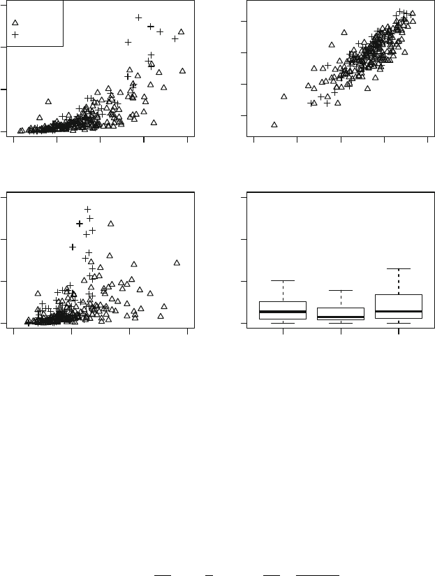
428 11 Positive Continuous Data: Gamma and Inverse Gaussian GLMs
010203040
0
5
10
15
DBH (in cm)
Foliage biomass (in kg)
l
l
l
l
l
l
l
l
l
l
l
l
l
l
l
l
l
l
l
l
l
l
l
ll
l
l
l
l
ll
l
l
l
l
l
l
l
l
l
l
ll
l
l
l
l
l
l
l
l
l
l
l
l
l
l
l
l
l
l
l
l
l
l
l
l
l
l
l
l
l
l
l
l
l
l
l
l
l
l
l
l
l
l
l
l
l
l
l
l
l
l
l
l
l
l
l
l
l
l
l
l
l
l
l
l
l
l
l
l
l
l
l
l
l
l
l
l
l
l
l
l
l
l
l
l
l
l
l
l
l
l
l
Coppice
Natural
Planted
01234
−4
−2
0
2
log of DBH (in cm)
log of Foliage biomass (in kg)
l
l
l
l
l
l
l
l
l
l
l
l
l
l
l
l
l
l
l
l
l
l
l
ll
l
l
l
l
ll
l
l
l
l
l
l
l
l
l
l
ll
l
l
l
l
l
l
l
l
l
l
l
l
l
l
l
l
l
l
l
l
l
l
l
l
l
l
l
l
l
l
l
l
l
l
l
l
l
l
l
l
l
l
l
l
l
l
l
l
l
l
l
l
l
l
l
l
l
l
l
l
l
l
l
l
l
l
l
l
l
l
l
l
l
l
l
l
l
l
l
l
l
l
l
l
l
l
l
l
l
l
0 50 100 150
0
5
10
15
Age (in years)
Foliage biomass (in kg)
l
l
l
l
l
l
l
l
l
l
l
l
l
l
l
l
l
l
l
l
l
l
l
ll
l
l
l
l
ll
l
l
l
l
l
l
l
l
l
l
ll
l
l
l
l
l
l
l
l
l
l
l
l
l
l
l
l
l
l
l
l
l
l
l
l
l
l
l
l
l
l
l
l
l
l
l
l
l
l
l
l
l
l
l
l
l
l
l
l
l
l
l
l
l
l
l
l
l
l
l
l
l
l
l
l
l
l
l
l
l
l
l
l
l
l
l
l
l
l
l
l
l
l
l
l
l
l
l
l
l
l
l
l
l
l
l
l
l
l
l
l
l
l
l
l
l
l
l
l
l
l
l
l
l
l
l
l
l
l
l
l
l
l
l
l
Coppice Natural Planted
0
5
10
15
Origin
Foliage biomass (in kg)
Fig. 11.1 The small-leaved lime data. Foliage biomass against dbh (diameter at breast
height; top left panel); log of foliage biomass against the log of dbh (diameter at breast
height; top right panel); foliage biomass against age (bottom left panel) foliage biomass
against origin (bottom right panel) (Example 11.1)
for y>0, α>0 (the shape parameter) and β>0 (the scale parameter),
where E[y]=αβ and var[y]=αβ
2
. Note that Γ () is the gamma function
(where, for example, if n is a non-negative integer then Γ (n)=(n − 1)!).
Writing in terms of μ and φ, the probability function becomes
P(y; μ, φ)=
y
φμ
1/φ
1
y
exp
−
y
φμ
1
Γ (1/φ)
for y>0, and μ>0andφ>0, where α =1/φ and β = μφ. Plots of some
example gamma probability functions are shown in Fig. 11.2. The variance
function for the gamma distribution is V (μ)=μ
2
.Thecoefficient of variation
is defined as the ratio of the variance to the mean squared, and is a mea-
sure of the relative variation in the data. Therefore, the gamma distribution
has a constant coefficient of variation, and consequently gamma glmsare
useful in situations where the coefficient of variation is (approximately) con-
stant. Useful information about the gamma distribution appears in Table 5.1
(p. 221).

11.3 The Gamma Distribution 429
Gamma density:
Mean: 0.75
y
Density
012345
Gamma density:
Mean: 1.0
y
Density
Variance: 1
Variance: 0.5
012345
Gamma density:
Mean: 2.0
y
Density
012345
Fig. 11.2 Some example gamma probability functions (Sect. 11.3)
l
l
l
l
l
l
l
l
l
l
−0.5 0.0 0.5 1.0 1.5
−1
0
1
2
log(group means)
log(group variance)
Fig. 11.3 The small-leaved limed data: the logarithm of group variances plotted against
the logarithm of the group means (Example 11.2)
Example 11.2. For the small-leaved lime data (Example 11.1; data set: lime),
the data can be split into smaller groups, and the mean and variance of each
group calculated. Then, Fig. 11.3 shows that the variance increases as the
mean increases:
> # Define age *groups*
> lime$AgeGrp <- cut(lime$Age, breaks=4 )
> # Now compute means and variances of each origin/age group:
> vr <- with( lime, tapply(Foliage, list(AgeGrp, Origin), "var" ) )
> mn <- with( lime, tapply(Foliage, list(AgeGrp, Origin), "mean" ) )
> # Plot
> plot( log(vr) ~ log(mn), las=1, pch=19,
xlab="log(group means)", ylab="log(group variance)")

430 11 Positive Continuous Data: Gamma and Inverse Gaussian GLMs
> mf.lm <- lm( c(log(vr)) ~ c(log(mn)) )
> coef( mf.lm )
(Intercept) c(log(mn))
-0.165002 1.706453
> abline( coef( mf.lm ), lwd=2)
The slope of the line is a little less than 2, so approximately
log(group variance) ∝ 2 × log(group mean).
Re-arranging shows the group variance is approximately proportional to
square of the group mean. In other words, V (μ) ≈ μ
2
which corresponds
to a gamma distribution (Sect. 5.3.6).
For the gamma distribution, φ is almost always unknown and therefore
must be estimated (Sect. 11.6.1), so likelihood ratio tests are based on F -tests
(Sect. 7.6.4). Two common situations exist where φ is known. In situations
where y follows a normal distribution, the sample variances can be modelled
using a chi-square distribution, which is a gamma distribution with φ =
2. Secondly, the exponential distribution (4.37), which has a history of its
own apart from its connection with the gamma distribution, is a gamma
distribution with φ = 1 (see Problem 11.17).
The unit deviance for the gamma distribution is
d(y, μ)=2
−log
y
μ
+
y −μ
μ
. (11.1)
The residual deviance D(y, ˆμ)=
n
i=1
w
i
d(y
i
, ˆμ
i
) ∼ χ
2
n−p
approximately, by
the saddlepoint approximation, for a model with p
parameters in the linear
predictor. The saddlepoint approximation is adequate if φ ≤ 1/3 (Sect. 7.5,
p. 276).
The canonical link function for the gamma distribution is the inverse (or
reciprocal) link function η =1/μ. In practice, the logarithmic link function is
often used because it avoids the need for constraints on the linear predictor
in view of μ>0. The log-link often also leads to a useful interpretation
where the impact of the explanatory variables is multiplicative (as discussed
in the context of Poisson glms; see Sect. 10.2). Other link functions are used
sometimes to produce desirable features (Sect. 11.5).
The gamma distribution can be used to describe the time between occur-
rences that follow a Poisson distribution. More formally, suppose an event
occurs over a time interval of length T at the Poisson rate of λ events per
unit time. Assuming the probability of more than one event in a very small
time interval is small, then the number of events in the interval from time 0
to time T can be modelled using a Poisson distribution. Then the length
of time y required for r events to occur follows a gamma distribution, with
mean r/λ and variance r/λ
2
. In this interpretation, r is an integer, which

11.4 The Inverse Gaussian Distribution 431
0 50 100 150
0
10
20
30
40
The cumulative number of events
over time
Time
Cumulative number of events
y = 45
y = 54
y = 18
0 20 40 60 80 100 120
0.000
0.005
0.010
0.015
0.020
0.025
0.030
Distribution of time y required to reach
r = 10 across 10000 simulations
Time required between
occurrence of 10 events
Density
Empirical
Gamma
Fig. 11.4 The gamma distribution describes the time between Poisson events. Left
panel: the occurrence of the Poisson events showing the time y between the occurrence
of r = 10 Poisson events for the first three occurrences only. Right panel: the distribution
of the time y between events has a gamma distribution (Example 11.3)
is not true in general for the gamma distribution. When r is an integer, the
gamma distribution is also called the Erlang distribution.
Example 11.3. Suppose events occur over a time interval of T = 1 at the rate
of λ =0.2 per unit time. The length of time y for r = 10 events to occurs
is shown in Fig. 11.4 (left panel) for the first three sets of r =10events.
The distribution of these times has an approximate gamma distribution with
mean r/λ =10/0.2 = 50 and variance r/λ
2
=10/0.2
2
= 250 (Fig. 11.4, right
panel).
11.4 The Inverse Gaussian Distribution
The inverse Gaussian distribution may sometimes be suitable for modelling
positive continuous data. The inverse Gaussian has the probability function
P(y; μ, φ)=(2πy
3
φ)
−1/2
exp
−
1
2φ
(y −μ)
2
yμ
2
(11.2)
where y>0, for μ>0 and the dispersion parameter φ>0. The variance
function is V (μ)=μ
3
. The inverse Gaussian distribution is used when the
responses are even more skewed than suggested by the gamma distribution.
Plots of some example inverse Gaussian densities are shown in Fig. 11.5.
The canonical link function for the inverse Gaussian distribution is
η = μ
−2
, though other link functions are almost always used in practice

432 11 Positive Continuous Data: Gamma and Inverse Gaussian GLMs
Inverse Gaussian density:
Mean: 0.75
y
Density
012345
Inverse Gaussian density:
Mean: 1.0
y
Density
Variance: 1
Variance: 0.5
012345
Inverse Gaussian density:
Mean: 2.0
y
Density
012345
Fig. 11.5 Some example inverse Gaussian probability functions (Sect. 11.4)
(Sect. 11.5), often to ensure μ>0 and for interpretation purposes. The unit
deviance for the inverse Gaussian distribution is
d(y, μ)=
(y −μ)
2
yμ
2
,
when the residual deviance is D(y, ˆμ)=
n
i=1
w
i
d(y
i
, ˆμ
i
), where the w
i
are
the prior weights. The unit deviance for the inverse Gaussian distribution is
distributed exactly as χ
2
1
(Sect. 5.4.3), since the saddlepoint approximation
is exact for the inverse Gaussian distribution (Problem 11.4). This means
D(y, ˆμ) ∼ χ
2
n−p
exactly (apart from sampling error in estimating μ
i
and φ)
for a model with p
parameters in the linear predictor. Useful information
about the inverse Gaussian distribution appears in Table 5.1 (p. 221). For
the inverse Gaussian distribution, φ is almost always unknown and estimated
(Sect. 11.6.2), so likelihood ratio tests are based on F -tests (Sect. 7.6.4).
The inverse Gaussian distribution has an interesting interpretation, con-
nected to Brownian motion. Brownian motion is the name given to the ran-
dom movement of particles over time. For a particle moving with Brown-
ian motion with positive drift (the tendency to move from the current loca-
tion), the inverse Gaussian distribution describes the distribution of the time
taken for the particle to reach some point that is a fixed positive distance
δ away. The normal distribution, also known as the Gaussian distribution,
describes the distribution of distance from the origin at fixed time. The in-
verse Gaussian distribution gets its name from this relationship to the normal
distribution.
To demonstrate these connections between the normal and inverse Gaus-
sian distribution in r, consider a particle moving with Brownian motion with
drift 0.5. We can measure both the time taken to exceed a fixed value δ =5
from the origin, and the distance of the particle from the origin after T = 20.

11.5 Link Functions 433
0 10203040
0
5
10
15
20
One realization of the
location of a particle
Time
Distance from origin
Threshold: 5
y = 7
010 30 50
0.00
0.02
0.04
0.06
0.08
0.10
Time taken to reach delta
across 1000 simulations
Time taken to reach threshold
Density
Empirical
Inv. Gaussian
l
l
l
l
l
l
l
l
l
l
l
l
l
l
l
l
l
l
l
l
l
l
l
l
l
l
l
l
l
l
l
l
l
l
l
l
l
l
l
l
l
l
l
l
l
l
l
l
l
l
l
l
l
l
l
l
l
l
l
l
l
l
l
l
l
l
l
l
l
l
l
l
l
l
l
l
l
l
l
l
l
l
l
l
l
l
l
l
l
l
l
l
l
l
l
l
l
l
l
l
l
l
l
l
l
l
l
l
l
l
l
l
l
l
l
l
l
l
l
l
l
l
l
l
l
l
l
l
l
l
l
l
l
l
l
l
l
l
l
l
l
l
l
l
l
l
l
l
l
l
l
l
l
l
l
l
l
l
l
l
l
l
l
l
l
l
l
l
l
l
l
l
l
l
l
l
l
l
l
l
l
l
l
l
l
l
l
l
l
l
l
l
l
l
l
l
l
l
l
l
l
l
l
l
l
l
l
l
l
l
l
l
l
l
l
l
l
l
l
l
l
l
l
l
l
l
l
l
l
l
l
l
l
l
l
l
l
l
l
l
l
l
l
l
l
l
l
l
l
l
l
l
l
l
l
l
l
l
l
l
l
l
l
l
l
l
l
l
l
l
l
l
l
l
l
l
l
l
l
l
l
l
l
l
l
l
l
l
l
l
l
l
l
l
l
l
l
l
l
l
l
l
l
l
l
l
l
l
l
l
l
l
l
l
l
l
l
l
l
l
l
l
l
l
l
l
l
l
l
l
l
l
l
l
l
l
l
l
l
l
l
l
l
l
l
l
l
l
l
l
l
l
l
l
l
l
l
l
l
l
l
l
l
l
l
l
l
l
l
l
l
l
l
l
l
l
l
l
l
l
l
l
l
l
l
l
l
l
l
l
l
l
l
l
l
l
l
l
l
l
l
l
l
l
l
l
l
l
l
l
l
l
l
l
l
l
l
l
l
l
l
l
l
l
l
l
l
l
l
l
l
l
l
l
l
l
l
l
l
l
l
l
l
l
l
l
l
l
l
l
l
l
l
l
l
l
l
l
l
l
l
l
l
l
l
l
l
l
l
l
l
l
l
l
l
l
l
l
l
l
l
l
l
l
l
l
l
l
l
l
l
l
l
l
l
l
l
l
l
l
l
l
l
l
l
l
l
l
l
l
l
l
l
l
l
l
l
l
l
l
l
l
l
l
l
l
l
l
l
l
l
l
l
l
l
l
l
l
l
l
l
l
l
l
l
l
l
l
l
l
l
l
l
l
l
l
l
l
l
l
l
l
l
l
l
l
l
l
l
l
l
l
l
l
l
l
l
l
l
l
l
l
l
l
l
l
l
l
l
l
l
l
l
l
l
l
l
l
l
l
l
l
l
l
l
l
l
l
l
l
l
l
l
l
l
l
l
l
l
l
l
l
l
l
l
l
l
l
l
l
l
l
l
l
l
l
l
l
l
l
l
l
l
l
l
l
l
l
l
l
l
l
l
l
l
l
l
l
l
l
l
l
l
l
l
l
l
l
l
l
l
l
l
l
l
l
l
l
l
l
l
l
l
l
l
l
l
l
l
l
l
l
l
l
l
l
l
l
l
l
l
l
l
l
l
l
l
l
l
l
l
l
l
l
l
l
l
l
l
l
l
l
l
l
l
l
l
l
l
l
l
l
l
l
l
l
l
l
l
l
l
l
l
l
l
l
l
l
l
l
l
l
l
l
l
l
l
l
l
l
l
l
l
l
l
l
l
l
l
l
l
l
l
l
l
l
l
l
l
l
l
l
l
l
l
l
l
l
l
l
l
l
l
l
l
l
l
l
l
l
l
l
l
l
l
l
l
l
l
l
l
l
l
l
l
l
l
l
l
l
l
l
l
l
l
l
l
l
l
l
l
l
l
l
l
l
l
l
l
l
l
l
l
l
l
l
l
l
l
l
l
l
l
l
l
l
l
l
l
l
l
l
l
l
l
l
l
l
l
l
l
l
l
l
l
l
l
l
l
l
l
l
l
l
l
l
l
l
l
l
l
l
l
l
l
l
l
l
l
l
l
l
l
l
l
l
l
l
l
l
l
l
l
l
l
l
l
l
l
l
l
l
l
l
l
l
l
l
l
l
l
l
l
l
l
l
l
l
l
l
l
l
l
l
l
l
l
l
l
l
l
l
l
l
l
l
l
l
l
l
l
l
l
l
l
l
l
l
l
l
l
l
l
l
l
l
l
l
l
l
l
l
l
l
l
l
l
l
l
l
l
l
l
l
l
l
l
l
l
l
l
l
l
l
l
l
l
l
l
l
l
l
l
l
l
l
l
l
l
l
l
l
l
l
l
l
l
l
l
l
l
l
l
l
l
l
l
l
l
l
l
l
l
l
l
l
l
l
l
l
l
l
l
l
l
l
l
l
l
l
l
l
l
l
l
l
l
l
l
l
l
l
l
l
l
l
l
l
l
l
l
l
l
l
l
l
l
l
l
l
l
l
l
l
l
l
l
l
l
l
l
l
l
l
l
l
l
l
l
l
l
l
l
l
l
l
l
l
l
l
l
l
l
l
l
l
l
l
l
l
l
l
l
l
l
l
l
l
l
l
l
l
l
l
l
l
l
l
l
l
l
l
l
l
l
l
l
l
l
l
l
l
l
l
l
l
l
l
l
l
l
l
l
l
l
l
l
l
l
l
l
l
l
l
l
l
l
l
l
l
l
l
l
l
l
l
l
l
l
l
l
l
l
l
l
l
l
l
l
l
l
l
l
l
l
l
l
l
l
l
l
l
l
l
l
l
l
l
l
l
l
l
l
l
l
l
l
l
l
l
l
l
l
l
l
l
l
l
l
l
l
l
l
l
l
l
l
l
l
l
l
l
l
l
l
l
l
l
l
l
l
l
l
l
l
l
l
l
l
l
l
l
l
l
l
l
l
l
l
l
l
l
l
l
l
l
l
l
l
l
l
l
l
l
l
l
l
l
l
l
l
l
l
l
l
l
l
l
l
l
l
l
l
l
l
l
l
l
l
l
l
l
l
l
l
l
l
ll
l
l
l
l
l
l
l
l
l
l
l
l
l
l
l
l
l
l
l
l
l
l
l
l
l
l
l
l
l
l
l
l
l
l
l
l
l
l
l
l
l
l
l
l
l
l
l
l
l
l
l
l
l
l
l
l
l
l
l
l
l
l
l
l
l
l
l
l
l
l
l
l
l
l
l
l
l
l
l
l
l
l
l
l
l
l
l
l
l
l
l
l
l
l
l
l
l
l
l
l
l
l
l
l
l
l
l
l
l
l
l
l
l
l
l
l
l
l
l
l
l
l
l
l
l
l
l
l
l
l
l
l
l
l
l
l
l
l
l
l
l
l
l
l
l
l
l
l
l
l
l
l
l
l
l
l
l
l
l
l
l
l
l
l
l
l
l
l
l
l
l
l
l
l
l
l
l
l
l
l
l
l
l
l
l
l
l
l
l
l
l
l
l
l
l
l
l
l
l
l
l
l
l
l
l
l
l
l
l
l
l
l
l
l
l
l
l
l
l
l
l
l
l
l
l
l
l
l
l
l
l
l
l
l
l
l
l
l
l
l
l
l
l
l
l
l
l
l
l
l
l
l
l
l
l
l
l
l
l
l
l
l
l
l
l
l
l
l
l
l
l
l
l
l
l
l
l
l
l
l
l
l
l
l
l
l
l
l
l
l
l
l
l
l
l
l
l
l
l
l
l
l
l
l
l
l
l
l
l
l
l
l
l
l
l
l
l
l
l
l
l
l
l
l
l
l
l
l
l
l
l
l
l
l
l
l
l
l
l
l
l
l
l
l
l
l
l
l
l
l
l
l
l
l
l
l
l
l
l
l
l
l
l
l
l
l
l
l
l
l
l
l
l
l
l
l
l
l
l
l
l
l
l
l
l
l
l
l
l
l
l
l
l
l
l
l
l
l
l
l
l
l
l
l
l
l
l
l
l
l
l
l
l
l
l
l
l
l
l
l
l
l
l
l
l
l
l
l
l
l
l
l
l
l
l
l
l
l
l
l
l
l
l
l
l
l
l
l
l
l
l
l
l
l
l
l
l
l
l
l
l
l
l
l
l
l
l
l
l
l
l
l
l
l
l
l
l
l
l
l
l
l
l
l
l
l
l
l
l
l
l
l
l
l
l
l
l
l
l
l
l
l
l
l
l
l
l
l
l
l
l
l
l
l
l
l
l
l
l
l
l
l
l
l
l
l
l
l
l
l
l
l
l
l
l
l
l
l
l
l
l
l
l
l
l
l
l
l
l
l
l
l
l
l
l
l
l
l
l
l
l
l
l
l
l
l
l
l
l
l
l
l
l
l
l
l
l
l
l
l
l
l
l
l
l
l
l
l
l
l
l
l
l
l
l
l
l
l
l
l
l
l
l
l
l
l
l
l
l
l
l
l
l
l
l
l
l
l
l
l
l
l
l
l
l
l
l
l
l
l
l
l
l
l
l
l
l
l
l
l
l
l
l
l
l
l
l
l
l
l
l
l
l
l
l
l
l
l
l
l
l
l
l
l
l
l
l
l
l
l
l
l
l
l
l
l
l
l
l
l
l
l
l
l
l
l
l
l
l
l
l
l
l
l
l
l
l
l
l
l
l
l
l
l
l
l
l
l
l
l
l
l
l
l
l
l
l
l
l
l
l
l
l
l
l
l
l
l
l
l
l
l
l
l
l
l
l
l
l
l
l
l
l
l
l
l
l
l
l
l
l
l
l
l
l
l
l
l
l
l
l
l
l
l
l
l
l
l
l
l
l
l
l
l
l
l
l
l
l
l
l
l
l
l
l
l
l
l
l
l
l
l
l
l
l
l
l
l
l
l
l
l
l
l
l
l
l
l
l
l
l
l
l
l
l
l
l
l
l
l
l
l
l
l
l
l
l
l
l
l
l
l
l
l
l
l
l
l
l
l
l
l
l
l
l
l
l
l
l
l
l
l
l
l
l
l
l
l
l
l
l
l
l
l
l
l
l
l
l
l
l
l
l
l
l
l
l
l
l
l
l
l
l
l
l
l
l
l
l
l
l
l
l
l
l
l
l
l
l
l
l
l
l
l
l
l
l
l
l
l
l
l
l
l
l
l
l
l
l
l
l
l
l
l
l
l
l
l
l
l
l
l
l
l
l
l
l
l
l
l
l
l
l
l
l
l
l
l
l
l
l
l
l
l
l
l
l
l
l
l
l
l
l
l
l
l
l
l
l
l
l
l
l
l
l
l
l
l
l
l
l
l
l
l
l
l
l
l
l
l
l
l
l
l
l
l
l
l
l
l
l
l
l
l
l
l
l
l
l
l
l
l
l
l
l
l
l
l
l
l
l
l
l
l
l
l
l
l
l
l
l
l
l
l
l
l
l
l
l
l
l
l
l
l
l
l
l
l
l
l
l
l
l
l
l
l
l
l
l
l
l
l
l
l
l
l
l
l
l
l
l
l
l
l
l
l
l
l
l
l
l
l
l
l
l
l
l
l
l
l
l
l
l
l
l
l
l
l
l
l
l
l
l
l
l
l
l
l
l
l
l
l
l
l
l
l
l
l
l
l
l
l
l
l
l
l
l
l
l
l
l
l
l
l
l
l
l
l
l
l
l
l
l
l
l
l
l
l
l
l
l
l
l
l
l
l
l
l
l
l
l
l
l
l
l
l
l
l
l
l
l
l
l
l
l
l
l
l
l
l
l
l
l
l
l
l
l
l
l
l
l
l
l
l
l
l
l
l
l
l
l
l
l
l
l
l
l
l
l
l
l
l
l
l
l
l
l
l
l
l
l
l
l
l
l
l
l
l
l
l
l
l
l
l
l
l
l
l
l
l
l
l
l
l
l
l
l
l
l
l
l
l
l
l
l
l
l
l
l
l
l
l
l
l
l
l
l
l
l
l
l
l
l
l
l
l
l
l
l
l
l
l
l
l
l
l
l
l
l
l
l
l
l
l
l
l
l
l
l
l
l
l
l
l
l
l
l
l
l
l
l
l
l
l
l
l
l
l
l
l
l
l
l
l
l
l
−2 0 2
−5
0
5
10
15
20
25
Q−Q plot of distribution
of location from origin
Theoretical Quantiles
Sample Quantiles
Fig. 11.6 The connection between Brownian motion, the inverse Gaussian distribution
and the normal distribution. Left panel: the location of the particle x
t
at time t;centre
panel: the distribution of the time taken for the particle to exceed δ = 5 follows an
inverse Gaussian distribution; right panel: the distance of the particle from the origin
after T = 20 follows a normal distribution (Sect. 11.4)
The distribution of the time taken closely resembles the expected inverse
Gaussian distribution (Fig. 11.6, centre panel), and the distance of the par-
ticle from the origin closely follows a normal distribution (Fig. 11.6, right
panel).
11.5 Link Functions
The logarithmic link function is the link function most commonly used for
gamma and inverse Gaussian glms, to ensure μ>0 and for interpretation
purposes (Sect. 10.2). For the gamma and inverse Gaussian distributions, r
permits the link functions "log", "identity" and "inverse" (the default
for the gamma distribution). The link function link="1/mu^2" is also per-
mitted for the inverse Gaussian distribution, and is the default (canonical)
link function.
Example 11.4. For the small-leaved lime data in Example 11.1 (data set:
lime), no turning points or asymptotes are evident. Consider using a gamma
distribution with a variety of link functions, starting with the commonly-used
logarithmic link function, and using the ideas developed in Example 11.1 for
the model:
> lime.log <- glm( Foliage ~ Origin * log(DBH), family=Gamma(link="log"),
data=lime)
434 11 Positive Continuous Data: Gamma and Inverse Gaussian GLMs
We next try the inverse link function:
> lime.inv <- update(lime.log, family=Gamma(link="inverse") )
Error: no valid set of coefficients has been found: please supply starting
values
In addition: Warning message:
In log(ifelse(y == 0, 1, y/mu)) : NaNs produced
Using the inverse link function produces error messages: r cannot find
suitable starting points (which may indicate a poor model). This is because
the inverse link function does not restrict μ to be positive. To help r find a
starting point for fitting the model, starting points may be supplied to glm()
on the scale of the data (using the input mustart) or on the scale of the
linear predictor (using the input etastart). For example, we can provide the
fitted values from lime.log as a starting point:
> lime.inv <- update(lime.log, family=Gamma(link="inverse"),
mustart=fitted(lime.log) )
Error: no valid set of coefficients has been found: please supply starting
values
In addition: Warning message:
In log(ifelse(y == 0, 1, y/mu)) : NaNs produced
The model still can not be fitted, so we do not consider this model further.
Finally, we try the identity link function:
> lime.id <- update(lime.log, family=Gamma(link="identity"),
mustart = fitted(lime.log) )
Error: no valid set of coefficients has been found: please supply starting
values
In addition: Warning message:
In log(ifelse(y == 0, 1, y/mu)) : NaNs produced
Warning messages are displayed when fitting the model with the identity link
function: the algorithm did not converge. Again, we could supply starting
values to the algorithm to see if this helps:
> lime.id <- update(lime.log, family=Gamma(link="identity"),
mustart=fitted(lime.log) )
Error: no valid set of coefficients has been found: please supply starting
values
In addition: Warning message:
In log(ifelse(y == 0, 1, y/mu)) : NaNs produced
The glm with the identity link function still does not converge, so we do not
consider this model any further. The inverse-link and identity-link models
are not very sensible in any case, given Fig. 11.1.
For the log-link model, standard residual plots (using quantile residuals [4])
show that the model seems appropriate (Fig. 11.7):

11.5 Link Functions 435
l
l
l
l
l
l
l
l
l
l
l
l
l
l
l
l
l
l
l
l
l
l
l
l
l
l
l
l
l
l
l
l
l
l
l
l
l
l
l
l
l
l
l
l
l
l
l
l
l
l
l
l
l
l
l
l
l
l
l
l
l
l
l
l
l
l
l
l
l
l
l
l
l
l
l
l
l
l
l
l
l
l
l
l
l
l
l
l
l
l
l
l
l
l
l
l
l
l
l
l
l
l
l
l
l
l
l
l
l
l
l
l
l
l
l
l
l
l
l
l
l
l
l
l
l
l
l
l
l
l
l
l
l
l
l
l
l
l
l
l
l
l
l
l
l
l
l
l
l
l
l
l
l
l
l
l
l
l
l
l
l
l
l
l
l
l
l
l
l
l
l
l
l
l
l
l
l
l
l
l
l
l
l
l
l
l
l
l
l
l
l
l
l
l
l
l
l
l
l
l
l
l
l
l
l
l
l
l
l
l
l
l
l
l
l
l
l
l
l
l
l
l
l
l
l
l
l
l
l
l
l
l
l
l
l
l
l
l
l
l
l
l
l
l
l
l
l
l
l
l
l
l
l
l
l
l
l
l
l
l
l
l
l
l
l
l
l
l
l
l
l
l
l
l
l
l
l
l
l
l
l
l
l
l
l
l
l
l
l
l
l
l
l
l
l
l
l
l
l
l
l
l
l
l
l
l
l
l
l
l
l
l
l
l
l
l
l
l
l
l
l
l
l
l
l
l
l
l
l
l
l
l
l
l
l
l
l
l
l
l
l
l
l
l
l
l
l
l
l
l
l
l
l
l
l
l
l
l
l
l
l
l
l
l
l
l
l
l
l
l
l
l
l
l
l
l
l
l
l
l
l
l
l
l
l
−3 −2 −1 0 1 2
−2
−1
0
1
2
3
4
Log link
Log of fitted values
Standardized residuals
l
l
l
l
l
l
l
l
l
l
l
l
l
l
l
l
l
l
l
l
l
l
l
l
l
l
l
l
l
l
l
l
l
l
l
l
l
l
l
l
l
l
l
l
l
l
l
l
l
l
l
l
l
l
l
l
l
l
l
l
l
l
l
l
l
l
l
l
l
l
l
ll
l
l
l
l
l
l
l
l
l
l
l
l
l
l
l
l
l
l
l
l
l
l
l
l
l
l
l
l
l
l
l
l
l
l
l
l
l
l
l
l
l
l
l
l
l
l
l
l
l
l
l
l
l
l
l
l
l
l
l
l
l
l
l
l
l
l
l
l
l
l
l
l
l
l
l
l
l
l
l
l
l
l
l
l
l
l
l
l
l
l
l
l
l
l
l
l
l
l
l
l
l
l
l
l
l
l
l
l
l
l
l
l
l
l
l
l
l
l
l
l
l
l
l
l
l
l
l
l
l
l
l
l
l
l
l
l
l
l
l
l
l
l
l
l
l
l
l
l
l
l
l
l
l
l
l
l
l
l
l
l
l
l
l
l
l
l
l
l
l
l
l
l
l
l
l
l
l
l
l
l
l
l
l
l
l
l
l
l
l
l
l
l
l
l
l
l
l
l
l
l
l
l
l
l
l
l
l
l
l
l
l
l
l
l
l
l
l
l
l
l
l
l
l
l
l
l
l
l
l
l
l
l
l
l
l
l
l
l
l
l
l
l
l
l
l
l
l
l
l
l
l
l
l
l
l
l
l
l
ll
l
l
l
l
l
l
l
l
l
l
l
l
l
l
l
l
l
l
l
l
l
l
l
l
l
l
l
l
l
l
l
l
l
l
l
l
l
l
l
l
l
l
l
l
l
l
l
l
l
l
l
l
−3 −2 −1 0 1 2
−4
−2
0
2
4
6
Linear predictor, eta
Working resid
l
l
l
l
l
l
l
l
l
l
l
l
l
l
l
l
l
l
l
l
l
l
l
l
l
l
l
l
l
l
l
l
l
l
l
l
l
l
l
l
l
l
l
l
l
l
l
l
l
l
l
l
l
l
l
l
l
l
l
l
l
l
l
l
l
l
l
l
l
l
l
l
l
l
l
l
l
l
l
l
l
l
l
l
l
l
l
l
l
l
l
l
l
l
l
l
l
l
l
l
l
l
l
l
l
l
l
l
l
l
l
l
l
l
l
l
l
l
l
l
l
l
l
l
l
l
l
l
l
l
l
l
l
l
l
l
l
l
l
l
l
l
l
l
l
l
l
l
l
l
l
l
l
l
l
l
l
l
l
l
l
l
l
l
l
l
l
l
l
l
l
l
l
l
l
l
l
l
l
l
l
l
l
l
l
l
l
l
l
l
l
l
l
l
l
l
l
l
l
l
l
l
l
l
l
l
l
l
l
l
l
l
l
l
l
l
l
l
l
l
l
l
l
l
l
l
l
l
l
l
l
l
l
l
l
l
l
l
l
l
l
l
l
l
l
l
l
l
l
l
l
l
l
l
l
l
l
l
l
l
l
l
l
l
l
l
l
l
l
l
l
l
l
l
l
l
l
l
l
l
l
l
l
l
l
l
l
l
l
l
l
l
l
l
l
l
l
l
l
l
l
l
l
l
l
l
l
l
l
l
l
l
l
l
l
l
l
l
l
l
l
l
l
l
l
l
l
l
l
l
l
l
l
l
l
l
l
l
l
l
l
l
l
l
l
l
l
l
l
l
l
l
l
l
l
l
l
l
l
l
l
l
l
l
l
l
l
l
l
l
l
l
l
l
l
l
l
l
l
l
l
l
l
l
l
−3 −2 −1 0 1 2 3
−2
−1
0
1
2
3
4
Normal Q−Q Plot
Theoretical Quantiles
Sample Quantiles
0 100 200 300 400
0.00
0.05
0.10
0.15
0.20
Index
Cook's distance
Fig. 11.7 Plots of the standardized residuals against the fitted values for two gamma
glms fitted to the small-leaved lime data. Left panels: using a logarithmic link function;
right panels: using an inverse link function; top panels: standardized residuals plotted
against log ˆμ; centre panels: the working residuals e plotted against ˆη; bottom panels:
Q–Q plots of the quantile residuals (Example 11.4)
> ## STDIZD RESIDUALS vs FITTED VALUES on constant-info scale
> plot(rstandard(lime.log) ~ log(fitted(lime.log)), main="Log link", las=1,
xlab="Log of fitted values", ylab="Standardized residuals")
> ## CHECK LINEAR PREDICTOR
> eta.log <- lime.log$linear.predictor
> plot(resid(lime.log, type="working") + eta.log ~ eta.log, las=1,
ylab="Working resid", xlab="Linear predictor, eta")
> ## QQ PLOT OF RESIDUALS
> qqnorm( qr1 <- qresid(lime.log), las=1 ); qqline( qr1 )
> ## COOK'S DISTANCE
> plot( cooks.distance(lime.log), ylab="Cook's distance", las=1, type="h")
Some observations produce large residuals, and some observations appear to
give a value of Cook’s distance larger than the others though none are deemed
influential:
> colSums(influence.measures(lime.log)$is.inf)
dfb.1_ dfb.OrgN dfb.OrgP dfb.l(DB dfb.ON:( dfb.OP:( dffit cov.r
000000729
cook.d hat
018

436 11 Positive Continuous Data: Gamma and Inverse Gaussian GLMs
0.0 1.0 2.0 3.0
10
20
30
40
50
log(μ) = 1 + x
x
μ
0.0 1.0 2.0 3.0
0.5
1.0
1.5
2.0
2.5
log(μ) = 1 − x
x
μ
0.0 1.0 2.0 3.0
20
40
60
80
100
log(μ) = 1 + x + 1 x
x
μ
0.0 1.0 2.0 3.0
0.0
0.1
0.2
0.3
log(μ) = 1 − x − 1 x
x
μ
0.0 1.0 2.0 3.0
0.0
0.5
1.0
1.5
2.0
log(μ) = 1 + 0.02x − 1 x
x
μ
0.0 1.0 2.0 3.0
5
10
15
20
log(μ) = 1 − 0.02x + 1 x
x
μ
Fig. 11.8 Various logarithmic link function relationships, based on [15, Figure 8.4]
(Sect. 11.5)
While the logarithmic link function is commonly used, judicious use of
the logarithmic and inverse link functions with transformations of covariates
accommodates a wide variety of relationships between the variables, including
data displaying asymptotes (Figs. 11.8 and 11.9). Polynomial relationships
cannot bound the value of μ, so non-polynomial linear predictors make more
physical sense in applications where asymptotes are present. Yield–density
experiments (Sect. 11.7.2) are one example where these relationships are used.
11.6 Estimating the Dispersion Parameter
11.6.1 Estimating φ for the Gamma Distribution
For the gamma distribution, the maximum likelihood estimate (mle)ofthe
dispersion parameter φ cannot be found in closed form. Defining the digamma
function as ψ(x)=Γ (x)
/Γ (x), the mle of φ is the solution to
D(y, ˆμ)=−2
n
i=1
w
i
log φ − w
i
log w
i
+ w
i
ψ(w
i
/φ) (11.3)
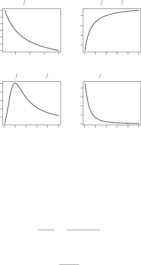
11.6 Estimating the Dispersion Parameter 437
1234
0.2
0.3
0.4
0.5
0.6
0.7
0.8
1 μ=1 + x
x
μ
0246810
0.2
0.4
0.6
0.8
1 μ=1 + 1 x
x
μ
0246810
0.1
0.2
0.3
0.4
0.5
1 μ=−2 + x + 4 x
x
μ
0246810
0.0
0.2
0.4
0.6
0.8
1 μ=1 + x + x
2
x
μ
Fig. 11.9 Various inverse link function relationships, based on [15, Figure 8.4])
(Sect. 11.5)
where D(y, ˆμ) is the residual deviance and n the sample size (Problem 11.1).
Solving (11.3)forφ requires iterative numerical methods. This is one reason
why the Pearson and deviance estimates are generally used.
Because the deviance is sensitive to very small values of y
i
for gamma
edms (Sect. 6.8.6), the Pearson estimator
¯
φ =
1
n − p
n
i=1
w
i
(y
i
− ˆμ
i
)
2
ˆμ
2
i
is recommended over the mean deviance estimator
˜
φ =
D(y, ˆμ)
n − p
for the gamma distribution when the accuracy of small values is in doubt,
for example when observations have been rounded to a limited number of
digits [15].
Example 11.5. Consider the gamma glm lime.log fitted in Example 11.4 to
the small-leaved lime data (data set: lime). Two estimates of φ are:
> phi.md <- deviance(lime.log)/df.residual(lime.log) # Mn dev estimate
> phi.pearson <- summary( lime.log )$dispersion # Pearson estimate
> c( "Mean Deviance"=phi.md, "Pearson"=phi.pearson)
438 11 Positive Continuous Data: Gamma and Inverse Gaussian GLMs
Mean Deviance Pearson
0.4028747 0.5443774
Using numerical methods (Problem 11.1), the mle is 0.3736.
Example 11.6. Using the model lime.log for the small-leaved lime data in
Example 11.1 (data set: lime), the analysis of deviance table is:
> round(anova(lime.log, test="F"), 3)
Df Deviance Resid. Df Resid. Dev F Pr(>F)
NULL 384 508.48
Origin 2 19.89 382 488.59 18.272 <2e-16 ***
log(DBH) 1 328.01 381 160.58 602.535 <2e-16 ***
Origin:log(DBH) 2 7.89 379 152.69 7.247 0.001 ***
---
Signif. codes: 0 '***' 0.001 '**' 0.01 '*' 0.05 '.' 0.1''1
By default, r uses the Pearson estimate of φ to produce this output. An F -
test is requested since φ is estimated. Other estimates of φ can be used also:
> round(anova(lime.log,test="F", dispersion=phi.md), 3)
Df Deviance Resid. Df Resid. Dev F Pr(>F)
NULL 384 508.48
Origin 2 19.89 382 488.59 24.690 < 2.2e-16 ***
log(DBH) 1 328.01 381 160.58 814.165 < 2.2e-16 ***
Origin:log(DBH) 2 7.89 379 152.69 9.793 < 2.2e-16 ***
---
Signif. codes: 0 '***' 0.001 '**' 0.01 '*' 0.05 '.' 0.1''1
The conclusions are very similar for either estimate of φ in this example.
Retaining all model terms, the parameter estimates are:
> printCoefmat(coef(summary(lime.log)), 3)
Estimate Std. Error t value Pr(>|t|)
(Intercept) -4.629 0.276 -16.79 <2e-16 ***
OriginNatural 0.325 0.388 0.84 0.4037
OriginPlanted -1.528 0.573 -2.67 0.0079 **
log(DBH) 1.843 0.102 18.15 <2e-16 ***
OriginNatural:log(DBH) -0.204 0.143 -1.42 0.1554
OriginPlanted:log(DBH) 0.577 0.209 2.76 0.0061 **
---
Signif. codes: 0 '***' 0.001 '**' 0.01 '*' 0.05 '.' 0.1''1
Notice that the reference level for Origin is Coppice, and that there is little
evidence of a difference between the natural and coppice trees. From the
model proposed in Example 11.1, the coefficient for dbh was expected to
be approximately 2; the estimate above is close to this value, and a formal
hypothesis tests could be conducted.

11.6 Estimating the Dispersion Parameter 439
11.6.2 Estimating φ for the Inverse Gaussian
Distribution
For the inverse Gaussian distribution, the mle of the dispersion parameter
is exactly (Problem 11.3)
ˆ
φ =
D(y, ˆμ)
n
.
As usual, the mle of φ is biased. However the mean deviance estimator
˜
φ =
D(y, ˆμ)
n − p
is essentially the same as the modified profile likelihood estimator, and is
very nearly unbiased. The mean deviance estimator has theoretically good
properties, and it recommended when good quality data is available. The
Pearson estimator is
¯
φ =
1
n − p
n
i=1
w
i
(y
i
− ˆμ
i
)
2
ˆμ
3
i
.
As with the gamma distribution, the deviance is sensitive to rounding errors
in very small values of y
i
(Sect. 6.8.6), so the Pearson estimator may be
better than mean deviance estimator when small values of y are recorded to
less than two significant figures. As always, the Pearson estimator is used in
r by default.
Example 11.7. For the small-leaved lime data (Example 11.1; data set: lime),
an inverse Gaussian glm could also be considered.
> lime.iG <- glm( Foliage ~ Origin * log(DBH),
family=inverse.gaussian(link="log"), data=lime)
The estimates of φ are:
> phi.iG.mle <- deviance(lime.iG)/length(lime$Foliage) # ML estimate
> phi.iG.md <- deviance(lime.iG)/df.residual(lime.iG) # Mean dev
> phi.iG.pearson <- summary( lime.iG )$dispersion # Pearson
> c( "MLE"=phi.iG.mle, "Mean dev."=phi.iG.md, "Pearson"=phi.iG.pearson)
MLE Mean dev. Pearson
1.056659 1.073387 1.255992
The aic suggests the gamma glm is preferred over the inverse Gaussian glm:
> c( "Gamma:"=AIC(lime.log), "inv. Gauss.:"=AIC(lime.iG) )
Gamma: inv. Gauss.:
750.3267 1089.5297

440 11 Positive Continuous Data: Gamma and Inverse Gaussian GLMs
11.7 Case Studies
11.7.1 Case Study 1
In a study of sheets of building materials [8, 12], the permeability of three
sheets was measured on three different machines over nine days, for a total of
81 sheets, all of equal thickness. Each measurement is an average permeabil-
ity of eight random pieces cut from each of the 81 sheets (Table 11.2; data
set: perm). The inverse Gaussian model may be appropriate: particles move
at random according to Brownian motion through the building material as-
suming uniform material, drifting across the sheet (Sect. 11.4). Plots of the
data (Fig. 11.10) show that the variance increases with the mean, and shows
one large observation that is a potential outlier:
> data(perm); perm$Day <- factor(perm$Day)
> boxplot( Perm ~ Day, data=perm, las=1, ylim=c(0, 200),
xlab="Day", ylab="Permeability (in s)")
> boxplot( Perm ~ Mach, data=perm, las=1, ylim=c(0, 200),
xlab="Machine", ylab="Permeability (in s)")
Because the inverse Gaussian distribution has a sensible interpretation
for these data, we adopt the inverse Gaussian model. We also select the
logarithmic link function, when the parameters are interpreted as having a
multiplicative effect on the response:
> perm.log <- glm( Perm ~ Mach * Day, data=perm,
family=inverse.gaussian(link="log") )
> round( anova( perm.log, test="F"), 3)
Df Deviance Resid. Df Resid. Dev F Pr(>F)
NULL 80 0.617
Mach 2 0.140 78 0.477 14.133 <2e-16 ***
Day 8 0.069 70 0.408 1.747 0.108
Table 11.2 The average permeability (in seconds) of eight sheets of building materials
(Sect. 11.7.1)
Machine Machine Machine
Day A B C Day A B C Day A B C
1 25.35 20.23 85.51 4 77.09 47.10 52.60 7 82.79 16.94 21.28
22.18 42.26 47.21 30.55 23.55 33.73 85.31 32.21 63.39
41.50 25.70 25.06 24.66 13.00 23.50 134.59 27.29 24.27
2 27.99 17.42 26.67 5 59.16 16.87 20.89 8 69.98 38.28 48.87
37.07 15.31 58.61 53.46 24.95 30.83 61.66 42.36 177.01
66.07 32.81 72.28 35.08 33.96 21.68 110.15 19.14 62.37
3 82.04 32.06 24.10 6 46.24 25.35 42.95 9 34.67 43.25 50.47
29.99 37.58 48.98 34.59 28.31 40.93 26.79 11.67 23.44
78.34 44.57 22.96 47.86 42.36 22.86 50.58 24.21 69.02

11.7 Case Studies 441
l
l
l
l
l
123456789
0
50
100
150
200
Day
Permeability (in s)
l
ABC
0
50
100
150
200
Machine
Permeability (in s)
Fig. 11.10 The permeability data. Permeability plotted against the day (left panel),
and permeability plotted against the machine (right panel) (Sect. 11.7.1)
Mach:Day 16 0.110 54 0.298 1.382 0.186
---
Signif. codes: 0 '***' 0.001 '**' 0.01 '*' 0.05 '.' 0.1''1
Recall the deviance has an exact distribution for the inverse Gaussian dis-
tribution, so these results do not rely on small-dispersion or large-sample
asymptotics. The interaction term is not necessary in the model. The effect
of Day is marginal, and so we omit Day from the model also.
> perm.log <- update( perm.log, Perm ~ Mach)
In this case, the model is simply modelling the means of these three machines:
> tapply( perm$Perm, perm$Mach, "mean") # Means from the data
ABC
54.65704 28.84963 45.98037
> tapply( fitted(perm.log), perm$Mach, "mean") # Fitted means
ABC
54.65704 28.84963 45.98037
The final model is:
> printCoefmat(coef(summary(perm.log)))
Estimate Std. Error t value Pr(>|t|)
(Intercept) 4.00108 0.11694 34.2137 < 2.2e-16 ***
MachB -0.63898 0.14455 -4.4205 3.144e-05 ***
MachC -0.17286 0.15868 -1.0894 0.2794
---
Signif. codes: 0 '***' 0.001 '**' 0.01 '*' 0.05 '.' 0.1''1
The model suggests the permeability measurements on Machine B are, on
average, exp(−0.6390) = 0.5278 times those for Machine A (the reference

442 11 Positive Continuous Data: Gamma and Inverse Gaussian GLMs
level). Likewise, the permeability measurements on Machine C are, on aver-
age, exp(−0.1729) = 0.8413 times those for Machine A. The output suggests
Machine C is very similar to Machine A, but Machine B is different.
We can now examine the fitted model to determine if the large observation
identified in Fig. 11.10 is an outlier, and if it is influential:
> range( rstudent(m1) )
[1] -2.065777 1.316577
> colSums(influence.measures(m1)$is.inf)
dfb.1_ dfb.x dffit cov.r cook.d hat
000200
No residuals appear too large. No observations are influential according to
Cook’s distance or dffits.
11.7.2 Case Study 2
Consider results from an experiment [16] to test the yields of three new
onion hybrids (Table 11.3; Fig. 11.11, left panel; data set: yieldden). This is
an example of a yield–density experiment [2, §17.3], [15, §8.3.3].
Yield per plant,sayz, and planting density, say x, usually exhibit an
inverse functional relationship such that
E[z]=
1
β
2
+ β
0
x + β
1
x
2
. (11.4)
Yield per unit area, y = xz, is usually of interest but is harder to measure
directly than yield per plant z. However,
μ =E[y]=xE[z]=
x
β
2
+ β
0
x + β
1
x
2
. (11.5)
Table 11.3 Plant yield density for an experiment with onion hybrids. The yields are
the mean yields per plant (in g); the density is in plants per square foot. The yields are
means over three plants, averaged on the log-scale (Example 11.7.2)
Variety 1 Variety 2 Variety 3
Yield Density Yield Density Yield Density
105.6 3.07 131.6 2.14 116.8 2.48
89.4 3.31 109.1 2.65 91.6 3.53
71.0 5.97 93.7 3.80 72.7 4.45
60.3 6.99 72.2 5.24 52.8 6.23
47.6 8.67 53.1 7.83 48.8 8.23
37.7 13.39 49.7 8.72 39.1 9.59
30.3 17.86 37.8 10.11 30.3 16.87
24.2 21.57 33.3 16.08 24.2 18.69
20.8 28.77 24.5 21.22 20.0 25.74
18.5 31.08 18.3 25.71 16.3 30.33

11.7 Case Studies 443
0 5 10 15 20 25 30
20
40
60
80
100
120
Yield per plant vs density
for onion growing experiment
Planting density (plants/sq. feet), x
Mean yield/plant (g/plant), z
l
l
l
l
l
l
l
l
l
l
l
Var. 1
Var. 2
Var. 3
0 5 10 15 20 25 30
300
350
400
450
500
550
600
Yield per unit area vs density
for onion growing experiment
Planting density (plants/sq. feet), x
Mean yield/area (g/sq. feet), y
l
l
l
l
l
l
l
l
l
l
l
Var. 1
Var. 2
Var. 3
Fig. 11.11 The yield–density onion data. Yield per plant z against planting density x
(left panel); yield per unit area y against planting density x (right panel) (Sect. 11.7.2)
Then inverting,
1
μ
= β
0
+ β
1
x + β
2
1
x
= η. (11.6)
The bottom left panel of Fig. 11.9 (p. 437) also shows this relationship be-
tween the two variables is appropriate: E[z] → 0asx →∞(that is, as the
planting density becomes very large the mean yield per plant diminishes) and
μ → 0asx → 0 (that is, as the planting density becomes almost zero the
mean yield per unit area diminishes). The plot of the mean yield per unit
area (Fig. 11.11, right panel) shows that as density increases, the yield per
unit area is more variable also. For this reason, we try using a gamma glm.
Hence, we model yield per unit area y using an inverse link function, with a
gamma edm:
> data(yieldden); yieldden$Var <- factor(yieldden$Var)
> yieldden$YD <- with(yieldden, Yield * Dens )
We adopt the theory-based model (11.6), adding interactions between the
terms involving Dens and Var to the model (note the use of the I() function).
> yd.glm.int <- glm( YD ~ (Dens + I(1/Dens)) * Var,
family=Gamma(link=inverse), data=yieldden )
> round( anova( yd.glm.int, test="F"), 2)
Df Deviance Resid. Df Resid. Dev F Pr(>F)
NULL 29 1.45
Dens 1 1.00 28 0.45 191.67 <2e-16 ***
I(1/Dens) 1 0.27 27 0.18 51.28 <2e-16 ***
Var 2 0.06 25 0.12 5.48 0.01 **
Dens:Var 2 0.01 23 0.12 0.57 0.57
I(1/Dens):Var 2 0.01 21 0.11 0.53 0.59
444 11 Positive Continuous Data: Gamma and Inverse Gaussian GLMs
---
Signif. codes: 0 '***' 0.001 '**' 0.01 '*' 0.05 '.' 0.1''1
None of the interaction terms are significant. Refit the model with no inter-
actions:
> yd.glm <- update( yd.glm.int, . ~ Dens + I(1/Dens) + Var )
> round( anova(yd.glm, test="F"), 2)
Df Deviance Resid. Df Resid. Dev F Pr(>F)
NULL 29 1.45
Dens 1 1.00 28 0.45 209.56 <2e-16 ***
I(1/Dens) 1 0.27 27 0.18 56.07 <2e-16 ***
Var 2 0.06 25 0.12 5.99 0.01 **
---
Signif. codes: 0 '***' 0.001 '**' 0.01 '*' 0.05 '.' 0.1''1
The fitted model is:
> printCoefmat( coef(summary(yd.glm)), 5)
Estimate Std. Error t value Pr(>|t|)
(Intercept) 1.9687e-03 1.3934e-04 14.1292 2.009e-13 ***
Dens -1.2609e-05 5.1637e-06 -2.4419 0.022026 *
I(1/Dens) 3.5744e-03 4.9364e-04 7.2409 1.376e-07 ***
Var2 1.0015e-04 7.1727e-05 1.3963 0.174914
Var3 2.4503e-04 7.1187e-05 3.4420 0.002041 **
---
Signif. codes: 0 '***' 0.001 '**' 0.01 '*' 0.05 '.' 0.1''1
While an optimal planting density (in terms of yield per unit area) can be
determined in principle (see Problem 11.6), Fig. 11.11 shows that the optimal
planting density is far beyond the range of the available data in this problem
so will probably be unreliable.
The diagnostics show that the model is adequate (Fig. 11.12):
> library(statmod) # For quantile residuals
> scatter.smooth( rstandard(yd.glm) ~ log(fitted(yd.glm)), las=1,
xlab="Log of fitted values", ylab="Standardized residuals" )
> plot( cooks.distance(yd.glm), type="h", las=1,
ylab="Cook's distance, D" )
> qqnorm( qr <- qresid(yd.glm), las=1 ); qqline(qr)
> plot( rstandard(yd.glm) ~ yieldden$Var, las=1,
xlab="Variety", ylab="Standardized residuals" )
The yield is modelled by a gamma distribution with the same dispersion
parameter for all values of the planting density and all varieties:
> summary(yd.glm)$dispersion
[1] 0.004789151
Since the estimate of φ is small, the saddlepoint approximation will be very
accurate (Sect. 7.5), and the distributional assumptions used in inferences are
accurate also (Sect. 5.4.4).
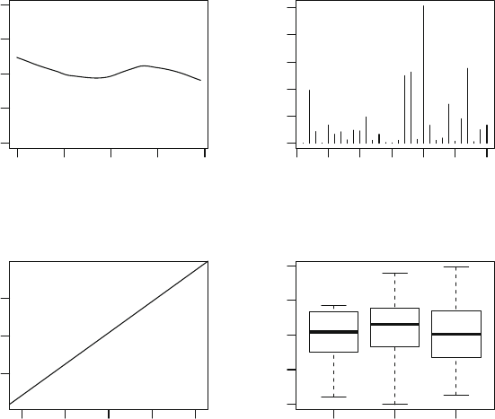
11.9 Summary 445
l
l
l
l
l
l
l
l
l
l
l
l
l
l
l
l
l
l
l
l
l
l
l
l
l
l
l
l
l
l
5.6 5.8 6.0 6.2 6.4
−2
−1
0
1
2
Log of fitted values
Standardized residuals
0 5 10 15 20 25 30
0.00
0.05
0.10
0.15
0.20
0.25
Index
Cook's distance, D
l
l
l
l
l
l
l
l
l
l
l
l
l
l
l
l
l
l
l
l
l
l
l
l
l
l
l
l
l
l
−2 −1 0 1 2
−1
0
1
Normal Q−Q Plot
Theoretical Quantiles
Sample Quantiles
123
−2
−1
0
1
2
Variety
Standardized residuals
Fig. 11.12 The diagnostic plots from fitting model yd.glm to the yield–density onion
data (Sect. 11.7.2)
11.8 Using R to Fit Gamma and Inverse Gaussian
GLMs
Gamma glms are specified in r using glm(formula, family=Gamma) in the
glm() call. (Note the capital G, since gamma() refers to the gamma func-
tion Γ ().) Inverse Gaussian glms are specified in r using glm(family=
inverse.gaussian) (note all lower case) in the glm() call. The link func-
tions "inverse", "identity" and "log" are permitted for both gamma and
inverse Gaussian distributions. The inverse Gaussian distribution also per-
mits the link function "1/mu^2" (the canonical link for the inverse Gaussian
distribution).
11.9 Summary
Chapter 11 considers fitting glms to positive continuous data. Positive
continuous data often have the variance increasing with increasing mean
(Sect. 11.2), so positive continuous data can be modelled using the gamma
446 11 Positive Continuous Data: Gamma and Inverse Gaussian GLMs
distribution (Sect. 11.3) or, for data more skewed than that suggested by the
gamma distribution, using the inverse Gaussian distribution (Sect. 11.4).
For the gamma distribution (Sect. 11.3), V (μ)=μ
2
. The residual deviance
D(y, ˆμ) is suitably described by a χ
2
n−p
distribution if φ ≤ 1/3. For the
inverse Gaussian distribution (Sect. 11.4), V (μ)=μ
3
. The residual deviance
D(y, ˆμ) is described by a χ
2
n−p
distribution.
The gamma distribution models the waiting time between events that
occur randomly according to a Poisson distribution (Sect. 11.3). The inverse
Gaussian distribution is related to the first-passage time in Brownian motion
(Sect. 11.4).
Commonly-used link functions are the logarithmic, inverse and identity
link functions (Sect. 11.5). Careful choice of the link function and transfor-
mations of the covariates can be used to describe asymptotic relationships
between y and x.
The Pearson estimate of φ is recommended for both the gamma and inverse
Gaussian distributions, though the mle of φ is exact for the inverse Gaussian
distribution (Sect. 11.6).
Problems
Selected solutions begin on p. 544.
11.1. Consider estimating φ for a gamma glm.
1. Prove the result (11.3)(p.436).
2. When w
i
= 1 for all observations i, show that the mle of φ is the solution
to D(y, ˆμ)=−2n{log φ + ψ(1/φ)}, where ψ(x)=Γ (x)
/Γ (x)isthe
digamma function.
3. Write an r function for computing the mle of φ for a gamma glm
with w
i
= 1 for all i.(Hint: The digamma function ψ(z) and the
trigamma function ψ
1
(z)=dψ(z)/dz are available in r as digamma()
and trigamma() respectively.)
4. Using this r function, find the mle of φ as given in Example 11.5 (p. 437).
11.2. If a fitted gamma glm includes a constant term and the logarithmic
link function is used, the sum over the observations of the second term
in the expression (11.1) for the residual deviance is zero. In other words,
n
i=1
(y
i
− ˆμ
i
)/ˆμ
i
= 0. Prove this result by writing the log-likelihood for a
model with linear predictor containing the constant term β
0
, differentiating
the log-likelihood with respect to β
0
, setting to zero and solving.
11.3. Show that the mle of the dispersion parameter φ for an inverse Gaus-
sian distribution is
ˆ
φ = D(y, ˆμ)/n.
11.4. In this problem we explore the distribution of the unit deviance for the
inverse Gaussian and gamma distributions.

11.9 Summary 447
1. Use r to generate 2000 random numbers y1 from an inverse Gaussian
distribution (using rinvgauss() from the statmod package [7, 26]) with
dispersion=0.1 (that is, φ =0.1). Fit an inverse Gaussian glm with
systematic component y1~1 and then compute the fitted unit deviances
d(y, ˆμ). By using qqplot(), show that these fitted unit deviances follow
a χ
2
1
distribution.
2. Use r to generate 2000 random numbers y2 from a gamma distribution
(using rgamma()) with shape=2 and scale=1. (This is equivalent to μ =2
and φ =1/2.) Fit a gamma glm with systematic component y2~1 and
then compute the fitted unit deviances d(y, ˆμ). By using qqplot(), show
that these fitted unit deviances do not follow a χ
2
1
distribution.
11.5. Consider the inverse Gaussian distribution (Table 5.1,p.221).
1. Show that the inverse Gaussian distribution with mean μ →∞(called
the Lévy distribution) has the probability function
P(y; φ)=
1
2πφy
3
exp{−1/(2yφ)} for y>0.
2. Show that the variance of the Lévy distribution is infinite.
3. Plot the Lévy probability function for φ =0.5andφ =2.
11.6. Show that the maximum value for μ for a gamma glm with a systematic
component of the form 1/μ = β
0
+ β
1
x + β
2
/x occurs at x =
β
2
/β
1
. Then,
show that this maximum value is μ =1/
β
0
+2
√
β
1
β
2
.
11.7. A study of insurance claims [19] modelled the amount of insurance
claims (for a total of 1975 claims) using a glm(gamma; log) model, with
five potential qualitative explanatory variables: policy-holder age P (five age
groups); vehicle type T (five types); vehicle age V (four age groups); district
D (five districts); and no-claims discount C (four levels). All main effects are
significant, and the interactions are tested using the deviance (Table 11.4).
1. Determine the changes in degrees of freedom after fitting each interaction
term.
2. Find an estimate of the dispersion parameter φ for the model with all
two-factor interactions.
3. Determine which interaction terms are significant using likelihood ratio
tests.
4. Interpret the meaning of the interaction term T.P.
11.8. The uk700 randomized trial [1] compared the 2-year costs (in dol-
lars) of treating mentally-ill patients in the community using two different
management approaches: intensive (caseload of 10–15 patients) and standard
(caseload of 30–35 patients). Data for 667 patients are available. Numerous
models were fitted, including those summarized in Table 11.5. For all these
models, g(μ)=β
0
+ β
1
x
1
+ β
2
x
2
, where x
1
= 1 for the intensive group and
is zero otherwise, and x
2
is the patient age in completed years.

448 11 Positive Continuous Data: Gamma and Inverse Gaussian GLMs
Table 11.4 The analysis of deviance table from fitting a gamma glm to claim severity
data; read down the columns (Problem 11.7)
Terms Residual deviance Terms Residual deviance
Main effects model 5050.9
+ T.P 4695.2 + P.D 4497.1
+ T.V 4675.9 + P.C 4462.0
+ T.D 4640.1 + V.D 4443.4
+ T.C 4598.8 + V.C 4420.8
+ P.V 4567.3 + D.C 4390.9
Table 11.5 Summaries of the glms fitted to the mental care cost data [1, Table 3],
using identity and logarithmic link functions (Problem 11.8)
edm g(μ)
ˆ
β
1
95% ci
ˆ
β
2
95% ci aic
Normal Identity 2032 (−1371, 5435) −3324 (−4812, −1836) 15, 259
Gamma Identity 1533 (−1746, 4813) −2622 (−3975, −1270) 14, 765
Inverse Gaussian Identity 1361 (−1877, 4601) −2416 (−3740, −1091) 15, 924
Normal Log 1.10 (0.95, 1.27) 0.84 (0.79, 0.90) 15, 256
Gamma Log 1.07 (0.93, 1.24) 0.88 (0.82, 0.93) 14, 763
Inverse Gaussian Log 1.07 (0.93, 1.23) 0.89 (0.84, 0.95) 15, 924
1. Based on the aic,whichedm seems most appropriate?
2. The constants in the models β
0
are not revealed. Nonetheless, write down
the two models based on this edm as comprehensively as possible.
3. Interpret the regression parameters for x
1
in both models.
4. Interpret the regression parameters for x
2
in both models.
5. Is the type of treatment significant for modelling cost? Explain.
6. Is the patient age significant for modelling cost? Explain.
7. Which interpretation (i.e. the use of which link function) seems most
appropriate? Why?
11.9. For the small-leaved lime data in data set lime, the gamma glm lime.
log was fitted in Example 11.6 (p. 438). Consider fitting a similar gamma
glm with a log link, but using DBH as the explanatory variable in place of
log(DBH).
1. Produce the diagnostic plots for this model.
2. Interpret the fitted model.
3. Do the diagnostic plots suggest which model (using DBH or log(DBH))is
preferred?
11.10. For the small-leaved lime data in data set lime, the model in
Example 11.1 proposed a relationship between Foliage and log(DBH).
Determine if a model that also includes Age improves the model.

11.9 Summary 449
Table 11.6 The average daily fat yields (in kg/day) each week for 35 weeks for a dairy
cow (Problem 11.12)
Week Yield Week Yield Week Yield Week Yield Week Yield
1 0.31 8 0.66 15 0.57 22 0.30 29 0.15
2 0.39 9 0.67 16 0.48 23 0.26 30 0.18
30.50 100.70 170.46 240.34 310.11
40.58 110.72 180.45 250.29 320.07
50.59 120.68 190.31 260.31 330.06
60.64 130.65 200.33 270.29 340.01
70.68 140.64 210.36 280.20 350.01
11.11. For the small-leaved lime data in data set lime, the model in
Example 11.1 proposed that the coefficient for log(DBH) was expected
to be approximately 2. For this problem, consider fitting a gamma glm with
only log(DBH) as an explanatory variable (that is, without Origin)totest
this idea.
1. Test this hypothesis using a Wald test, and comment.
2. Test this hypothesis using a likelihood ratio test, and comment.
11.12. In the dairy science literature, Wood’s lactation curve is the equation,
justified biometrically, relating the production of milk fat y in week t:
y = at
b
exp(ct),
where the parameters a, b and c are estimated from the data. Lactation
data [10] from one dairy cow are shown in Table 11.6 (data set: lactation).
1. Plot the data, and propose possible models based on the graphs shown
in Sect. 11.5.
2. Fit models suggested above, plus the model suggested by Wood’s lacta-
tion curve.
3. Plot the curves on the data, and comment.
11.13. A study of computer tomography (ct) interventions [23, 32] in the ab-
domen measured the total procedure time (in s) and the total radiation dose
received (in rads) (Table 3.21; data set: fluoro). During these procedures,
“one might postulate that the radiation dose received is related to. . . the total
procedure time” [32, p. 61].
1. Find a suitable glm for the data, ensuring a diagnostic analysis, and test
the hypothesis implied by the above quotation.
2. Plot the fitted model, including the 95% confidence interval about the
fitted line.
11.14. Nambe Mills, Santa Fe, New Mexico [3, 25], is a tableware manu-
facturer. After casting, items produced by Nambe Mills are shaped, ground,

450 11 Positive Continuous Data: Gamma and Inverse Gaussian GLMs
buffed, and polished. In 1989, as an aid to rationalizing production of its 100
products, the company recorded the total grinding and polishing times and
the diameter of each item (Table 5.3; data set: nambeware). In Chaps. 5–8
(Problems 5.26, 6.11, 7.5 and 8.12), only the item diameter was considered
as an explanatory variable. Now, consider modelling price y as a function of
all explanatory variables.
1. Plot the Price against Type, against Diam and against Time.Whatdothe
plots suggest about the relationship between the mean and the variance
for the data?
2. What possible distribution could be used to fit a glm? Justify your an-
swer.
3. Determine a good model for Price, considering interactions. Perform a
comprehensive diagnostic test of your model and comment on the struc-
ture of the fitted model.
4. Write down your final model(s).
5. Interpret your final model(s).
11.15. The lung capacity data [13] in Example 1.1 have been used in Chaps. 2
and 3 (data set: lungcap).
1. Plot the data, and identify possible relationships between FEV and the
other variables.
2. Find a suitable glm for the data, ensuring a diagnostic analysis.
3. Is there evidence that smoking affects lung capacity?
4. Interpret your model.
11.16. In a study of foetal size [20], the mandible length (in mm) and gesta-
tional age (in weeks) for 167 foetuses were measured from the 12th week
of gestation onwards (Table 11.7; data set: mandible). According to the
source [20, p. 437], the data for foetuses aged over 28 weeks should be dis-
carded, because “the technique was difficult to perform and excessive mea-
surement error was suspected”.
1. Using the subset() command in r, create a data frame of the measure-
ments for the 158 foetuses less than or equal to 28 weeks.
Table 11.7 The mandible length and foetal age (Problem 11.16)
Age (in weeks) Length (in mm)
12.3 8
12.4 9
12.7 11
12.7 11
12.9 10
.
.
.
.
.
.

11.9 Summary 451
2. Plot this data subset, and identify the important features of the data.
3. Fit a suitable model for the data subset. Consider exploring different link
functions, and including polynomial terms in age.
4. Plot the full data set (including foetuses older than 28 weeks of age), and
then draw the systematic component on the same plot. Does the model
fit well to these extra observations?
5. Find and interpret the 90% Wald confidence interval for the age param-
eter.
11.17. The times to death (in weeks) of two groups of leukaemia patients
whose white blood cell counts were measured (Table 4.3; data set: leukwbc)
were grouped according to a morphological variable called the ag factor [5].
1. Plot the survival time against white blood cell count (wbc), distinguish-
ing between ag-positive and ag-negative patients. Comment on the re-
lationship between wbc and survival time, and the ag factor.
2. Plot the survival time against log
10
wbc, and argue that using log
10
wbc
is likely to be a better choice as an explanatory variable.
3. Fit a glm(gamma; log) model to the data, including the interaction term
between the ag factor and log
10
wbc, and show that the interaction term
is not necessary.
4. Refit the glm without the interaction term, and evaluate the model using
diagnostic tools.
5. Plot the fitted lines for each ag-factor on a plot of the observations.
6. The original source [5] uses an exponential distribution (4.37), which is
a gamma distribution with φ = 1. Does this seem reasonable?
11.18. The data in Table 11.8 come from a study [14] of the nitrogen content
of soil, with three replicates at each dose (data set: nitrogen).
1. Plot the data, identifying the organic nitrogen source.
Table 11.8 The soil nitrogen (in kilograms of nitrogen per hectare) after applying
different doses of fertilizer (in kilograms of nitrogen per hectare). The fertilizers are in-
organic apart from the dose of 248 kg N ha
−1
, whose source is organic (farmyard manure)
(Problem 11.18)
Fertilizer dose Soil N content
Control 4.53 5.46 4.77
48 6.17 9.30 8.29
96 11.30 16.58 16.24
144 24.61 18.20 30.03
192 21.94 29.24 27.43
240 46.74 38.87 44.07
288 57.74 45.59 39.77
248 25.28 21.79 19.75

452 11 Positive Continuous Data: Gamma and Inverse Gaussian GLMs
2. Find the mean and variance of each fertilizer dose. Then, plot the loga-
rithm of the variance against the logarithm of the means, and show that
a gamma distribution appears sensible.
3. Fit a suitable gamma glm to the data, including a diagnostic analysis.
11.19. In Problem 2.18 (p. 88), data are given from an experiment where
children were asked to build towers out of cubical and cylindrical blocks as
high as they could [11, 24]. The number of blocks used and the time taken
were recorded (Table 2.12; data set: blocks). In this problem, we examine
the time taken to stack blocks.
1. Find a suitable gamma glm for modelling the time taken to build the
towers.
2. Find a suitable inverse Gaussian glm for modelling the time taken to
build the towers.
3. Using a diagnostic analysis, determine which of the two models is more
appropriate.
4. Test the hypothesis that the time taken to stack the blocks differs between
cubical and cylindrical shaped blocks.
5. Test the hypothesis that older children take less time to stack the blocks,
for both cubes and cylinders.
11.20. Hardness of timber is difficult to measure directly, but is related to
the density of the timber (which is easier to measure). To study this rela-
tionship [29], density and Janka hardness measurements for 36 Australian
eucalyptus hardwoods were obtained (Table 11.9; data set: hardness). Ven-
ables [27] suggests that a glm using a square-root link function with a gamma
distribution fits the data well. Fit the suggested model, and use a diagnostic
analysis to show that this model seems reasonable.
Table 11.9 The Janka hardness and density of Australian hardwoods, units unknown
(Problem 11.20)
Density Hardness Density Hardness Density Hardness
24.7 484 39.4 1210 53.4 1880
24.8 427 39.9 989 56.0 1980
27.3 413 40.3 1160 56.5 1820
28.4 517 40.6 1010 57.3 2020
28.4 549 40.7 1100 57.6 1980
29.0 648 40.7 1130 59.2 2310
30.3 587 42.9 1270 59.8 1940
32.7 704 45.8 1180 66.0 3260
35.6 979 46.9 1400 67.4 2700
38.5 914 48.2 1760 68.8 2890
38.8 1070 51.5 1710 69.1 2740
39.3 1020 51.5 2010 69.1 3140
11.9 Summary 453
11.21. In Problem 3.19, a study of urethral length L and mass M of various
mammals [30] was discussed. For these data (data set: urinationL), one
postulated relationship is L = kM
1/3
for some proportionality constant k.
In that Problem, a weighted regression model was fitted to the data using a
transformation of the relationship to linearity: log L = log k + (log M)/3. Fit
an approximately-equivalent glm for modelling these data. Using this model,
test the hypothesis again using both a Wald and likelihood-ratio test.
11.22. In Problem 3.11 (p. 150), data are given from a study of the food
consumption of fish [17] (data set: fishfood). In Problem 3.11, the linear
regression model fitted in the source is shown. Fit the equivalent gamma
glm for modelling the daily food consumption, and compare to the linear
regression model in Problem 3.11.
11.23. In Problem 3.17, the daily energy requirements [9, 28, 31] and weight
of 64 wethers (Table 2.11; data set: sheep) were analysed using a linear
regression model, using the logarithm of the daily energy requirements as the
response.
1. Fit the equivalent glm.
2. Perform a diagnostic analysis of the glm and compare to the regres-
sion model using the logarithm of the daily energy requirements as the
response. Comment.
3. Plot the data and the fitted glm, and add the 95% confidence intervals
for the fitted values.
4. Interpret the glm.
11.24. An experiment to investigate the initial rate of benzene oxidation [18]
over a vanadium oxide catalyst used three different reaction temperatures and
varied oxygen and benzene concentrations. A subset of the data is presented
in Table 11.10 (data set: rrates) for a benzene concentration near 2 ×10
−3
gmoles/L.
1. Plot the reaction rate against oxygen concentration, distinguishing dif-
ferent temperatures. What important features of the data are obvious?
2. Compare the previous plot to Fig. 11.8 (p. 436) and Fig. 11.9 (p. 437).
Suggest two functional relationships between oxygen concentration and
reaction rate that could be compared.
3. Fit the models identified above, and separately plot the fitted systematic
components on the data. Select a model, explaining your choice.
4. For your chosen model, perform a diagnostic analysis, identifying poten-
tial problems with the model.
5. By looking at the data for each temperature separately, is it reasonable to
assume the dispersion parameter φ is approximately constant? Explain.

454 REFERENCES
Table 11.10 The initial reaction rate of benzene oxidation. Oxygen concentration [O]
is ×10
4
gmole/L; the temperature is in Kelvin; and the reaction rate is ×10
19
gmole/g
of catalyst/s (Problem 11.24)
Temp: 623 K Temp: 648 K Temp: 673 K
[O] Rate [O] Rate [O] Rate
134.5 218 23.3 229 16.0 429
108.0 189 40.8 296 23.5 475
68.6 192 140.3 547 132.8 1129
49.5 174 140.8 582 107.7 957
41.7 152 141.2 480 68.5 745
29.4 139 140.0 493 47.2 649
22.5 118 121.2 513 42.5 742
17.2 120 104.7 411 30.1 662
17.0 122 40.8 349 11.2 373
22.8 132 22.5 226 17.1 440
41.3 167 55.2 338 65.8 662
59.6 208 55.4 351 108.2 724
119.7 216 29.5 295 123.5 915
158.2 294 30.0 294 160.0 944
16.3 233 66.4 713
16.5 222 66.5 736
20.8 239
20.6 217
References
[1] Barber, J., Thompson, S.: Multiple regression of cost data: Use of gen-
eralized linear models. Journal of Health Services Research and Policy
9(4), 197–204 (2004)
[2] Crawley, M.J.: Glim for Ecologists. Blackwell Scientific Publications,
London (1993)
[3] Data Desk: Data and story library (dasl) (2017). URL http://dasl.
datadesk.com
[4] Dunn, P.K., Smyth, G.K.: Randomized quantile residuals. Journal of
Computational and Graphical Statistics 5(3), 236–244 (1996)
[5] Feigl, P., Zelen, M.: Estimation of exponential survival probabilities with
concomitant information. Biometrics 21, 826–838 (1965)
[6] Fox, R., Garbuny, M., Hooke, R.: The Science of Science. Walker and
Company, New York (1963)
[7] Giner, G., Smyth, G.K.: statmod: probability calculations for the inverse
Gaussian distribution. The R Journal 8(1), 339–351 (2016)
[8] Hald, A.: Statistical Theory with Engineering Applications. John Wiley
and Sons, New York (1952)
[9] Hand, D.J., Daly, F., Lunn, A.D., McConway, K.Y., Ostrowski, E.: A
Handbook of Small Data Sets. Chapman and Hall, London (1996)
REFERENCES 455
[10] Henderson, H.V., McCulloch, C.E.: Transform or link? Tech. Rep. BU-
049-MA, Cornell University (1990)
[11] Johnson, B., Courtney, D.M.: Tower building. Child Development 2(2),
161–162 (1931)
[12] Jørgensen, B.: Exponential dispersion models and extensions: A review.
International Statistical Review 60(1), 5–20 (1992)
[13] Kahn, M.: An exhalent problem for teaching statistics. Journal of Sta-
tistical Education 13(2) (2005)
[14] Lane, P.W.: Generalized linear models in soil science. European Journal
of Soil Science 53, 241–251 (2002)
[15] McCullagh, P., Nelder, J.A.: Generalized Linear Models, second edn.
Monographs on Statistics and Applied Probability. Chapman and Hall,
London (1989)
[16] Mead, R.: Plant density and crop yield. Applied Statistics 19(1), 64–81
(1970)
[17] Palomares, M.L., Pauly, D.: A multiple regression model for predicting
the food consumption of marine fish populations. Australian Journal of
Marine and Freshwater Research 40(3), 259–284 (1989)
[18] Pritchard, D.J., Downie, J., Bacon, D.W.: Further consideration of het-
eroscedasticity in fitting kinetic models. Technometrics 19(3), 227–236
(1977)
[19] Renshaw, A.E.: Modelling the claims process in the presence of covari-
ates. ASTIN Bulletin 24(2), 265–285 (1994)
[20] Royston, P., Altman, D.G.: Regression using fractional polynomials of
continuous covariates: Parsimonious parametric modelling. Journal of
the Royal Statistical Society, Series C 43(3), 429–467 (1994)
[21] Schepaschenko, D., Shvidenko, A., Usoltsev, V.A., Lakyda, P., Luo, Y.,
Vasylyshyn, R., Lakyda, I., Myklush, Y., See, L., McCallum, I., Fritz,
S., Kraxner, F., Obersteiner, M.: Biomass plot data base. PANGAEA
(2017). DOI 10.1594/PANGAEA.871465. In supplement to: Schep-
aschenko, D et al. (2017): A dataset of forest biomass structure for
Eurasia. Scientific Data, 4, 170070, doi:10.1038/sdata.2017.70
[22] Schepaschenko, D., Shvidenko, A., Usoltsev, V.A., Lakyda, P., Luo, Y.,
Vasylyshyn, R., Lakyda, I., Myklush, Y., See, L., McCallum, I., Fritz,
S., Kraxner, F., Obersteiner, M.: A dataset of forest biomass structure
for Eurasia. Scientific Data 4, 1–11 (2017)
[23] Silverman, S.G., Tuncali, K., Adams, D.F., Nawfel, R.D., Zou, K.H.,
Judy, P.F.: ct fluoroscopy-guided abdominal interventions: Techniques,
results, and radiation exposure. Radiology 212, 673–681 (1999)
[24] Singer, J.D., Willett, J.B.: Improving the teaching of applied statistics:
Putting the data back into data analysis. The American Statistician
44(3), 223–230 (1990)
[25] Smyth, G.K.: Australasian data and story library (Ozdasl) (2011).
URL http://www.statsci.org/data
456 REFERENCES
[26] Smyth, G.K.: statmod: Statistical Modeling (2017). URL https://
CRAN.R-project.org/package=statmod. R package version 1.4.30. With
contributions from Yifang Hu, Peter Dunn, Belinda Phipson and Yun-
shun Chen.
[27] Venables, W.N.: Exegeses on linear models. In: S-Plus User’s Conference.
Washington DC (1998). URL https://www.stats.ox.ac.uk/pub/MASS3/
Exegeses.pdf
[28] Wallach, D., Goffinet, B.: Mean square error of prediction in models for
studying ecological systems and agronomic systems. Biometrics 43(3),
561–573 (1987)
[29] Williams, E.J.: Regression Analysis. Wiley, New York (1959)
[30] Yang, P.J., Pham, J., Choo, J., Hu, D.L.: Duration of urination does not
change with body size. Proceedings of the National Academy of Sciences
111(33), 11 932–11 937 (2014)
[31] Young, B.A., Corbett, J.L.: Maintenance energy requirement of grazing
sheep in relation to herbage availability. Australian Journal of Agricul-
tural Research 23(1), 57–76 (1972)
[32] Zou, K.H., Tuncali, K., Silverman, S.G.: Correlation and simple linear
regression. Radiology 227, 617–628 (2003)

Chapter 12
Tweedie GLMs
...we cannot know if any statistical technique that we
develop is useful unless we use it.
Box [5, p. 792]
12.1 Introduction and Overview
This chapter introduces glms based on Tweedie edms. Tweedie edm sare
distributions that generalize many of the edms already seen (the normal,
Poisson, gamma and inverse Gaussian distributions are special cases) and
include other distributions also. First, Tweedie edms are discussed in general
(Sect. 12.2), and then two subsets of the Tweedie glms which are impor-
tant are studied: Tweedie edms for modelling positive continuous data for
which gamma and inverse Gaussian glms are special cases (Sect. 12.2.3), then
Tweedie edms for modelling continuous data with exact zeros (Sect. 12.2.4).
We then follow with a description of how to use these Tweedie edmstofit
Tweedie glms (Sect. 12.3).
12.2 The Tweedie EDMs
12.2.1 Introducing Tweedie Distributions
Apart from the binomial and negative binomial distributions, the edms seen
so far in this book have variance functions with similar forms:
• the normal distribution, where V (μ)=μ
0
= 1 (Chaps. 2 and 3);
• the Poisson distribution, where V (μ)=μ
1
(Chap. 10);
• the gamma distribution, where V (μ)=μ
2
(Chap. 11);
• the inverse Gaussian distribution, where V (μ)=μ
3
(Chap. 11).
These edms have power variance functions of the form V (μ)=μ
ξ
, with
ξ =0, 1, 2, 3. More generally, any edm with a variance function V (μ)=μ
ξ
is
called a Tweedie distribution,oraTweedie edm, where ξ can take any real
© Springer Science+Business Media, LLC, part of Springer Nature 2018
P. K. Dunn, G. K. Smyth, Generalized Linear Models with Examples in R,
Springer Texts in Statistics, https://doi.org/10.1007/978-1-4419-0118-7_12
457

458 12 Tweedie GLMs
Table 12.1 Features of the Tweedie distributions for various values of the index param-
eter ξ, showing the support S (the permissible values of y) and the domain Ω for μ.The
Poisson distribution (ξ =1andφ = 1) is a special case of the discrete distributions, and
the inverse Gaussian distribution (ξ = 3) is a special case of positive stable distributions.
R refers to the real line; superscript + means positive real values only; subscript 0 means
zero is included in the space (Sect. 12.2.1)
Tweedie edm ξSΩReference
Extreme stable ξ<0 RR
+
Not covered
Normal ξ =0 RRChaps. 2 and 3
No edmsexist 0<ξ<1
Discrete ξ =1 y =0,φ,2φ,... R
+
Chap. 10 for φ =1
Poisson-gamma 1 <ξ<2 R
+
0
R
+
Sect. 12.2.3
Gamma ξ =2 R
+
R
+
Chap. 11
Positive stable ξ>2 R
+
R
+
Sect. 12.2.4
value except 0 <ξ<1[25]. ξ is called the Tweedie index parameter and is
sometimes denoted by p. This power-variance relationship has been observed
in natural populations for many years [36, 37]. Useful information about the
Tweedie distribution appears in Table 5.1 (p. 221).
The four specific cases of Tweedie distributions listed above show that the
Tweedie distributions are useful for a variety of data types (Table 12.1). More
generally:
•Forξ ≤ 0, the Tweedie distributions are suitable for modelling continuous
data where −∞ <y<∞. The normal distribution (ξ = 0) is a special
case. When ξ<0, the Tweedie distributions have the unusual feature
that data y are defined on the entire real line, but μ>0. These Tweedie
distributions with ξ<0 have no known realistic applications, and so are
not considered further.
•Forξ = 1 the Tweedie distributions are suitable for modelling discrete
data where y =0,φ,2φ, 3φ,.... When φ = 2, for example, a positive
probability exists for y =0, 2, 4,.... The Poisson distribution is a special
case when φ =1.
•For1<ξ<2, the Tweedie distributions are suitable for modelling
positive continuous data with exact zeros. An example is rainfall mod-
elling [12, 31]: when no rain falls, an exact zero is recorded, but when
rain does fall, the amount is a continuous measurement. Plots of example
probability functions are shown in Fig. 12.1.Asξ → 1, the densities show
local maxima corresponding to the discrete masses for the corresponding
Poisson distribution.
•Forξ ≥ 2, the Tweedie distributions are suitable for modelling positive
continuous data. The gamma (
ξ = 2) and inverse Gaussian (ξ =3)
distributions are special cases (Chap. 11). The distributions become more
right skewed as ξ increases (Fig. 12.2).
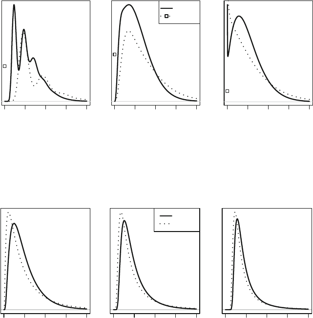
12.2 The Tweedie EDMs 459
ξ=1.05
y
Density
l
l
01234
ξ=1.2
y
Density
l
01234
l
φ=0.5
φ=1
ξ=1.6
y
Density
l
01234
Fig. 12.1 Examples of Tweedie probability functions with 1 <ξ<2andμ =1.The
solid lines correspond to φ =0.5 and the dotted lines to φ = 1. The filled dots show the
probability of exactly zero when φ =0.5 and the empty squares show the probability of
exactly zero when φ = 1 (Sect. 12.2.1)
ξ=2.5
y
Density
01234
ξ=3.5
y
Density
01234
φ=0.5
φ=1
ξ=5
y
Density
01234
Fig. 12.2 Examples of Tweedie probability functions with ξ>2andμ =1.Asξ gets
larger, the distributions become more skewed to the right. The solid lines correspond to
φ =0.5; the dotted lines to φ = 1 (Sect. 12.2.1)
ξ is called the Tweedie index parameter for the Tweedie distributions, and
specifies the particular distribution in the Tweedie family of distributions.
The two cases 1 <ξ<2andξ ≥ 2 are considered in this chapter in further
detail. (The special cases ξ =0, 1, 2, 3 were considered earlier.)

460 12 Tweedie GLMs
12.2.2 The Structure of Tweedie EDMs
Tweedie distributions are defined as edms with variance function V (μ)=μ
ξ
for some given ξ. Using this relationship, θ and κ(θ) can be determined (fol-
lowing the ideas in Sect. 5.3.6). Setting the arbitrary constants of integration
to zero, obtain (Problem 12.1)
θ =
⎧
⎪
⎨
⎪
⎩
μ
1−ξ
1 − ξ
for ξ =1
log μ for ξ =1
and κ(θ)=
⎧
⎪
⎨
⎪
⎩
μ
2−ξ
2 − ξ
for ξ =2
log μ for ξ =2
. (12.1)
Other parameterizations are obtained by setting the constants of integration
to other values. One useful parameterization ensures θ and κ(θ) are con-
tinuous functions of ξ [16] (Problem 12.2). The expressions for θ and κ(θ)
contain ξ, so the Tweedie distributions are only edmsifξ is known. In prac-
tice, the value of ξ is usually estimated (Sect. 12.3.2). If y follows a Tweedie
distribution with index parameter ξ, mean μ and dispersion parameter φ,
write y ∼ Tw
ξ
(μ, φ).
Based on these expressions for θ and κ(θ), the Tweedie probability function
may be written in canonical form (5.1). Apart from the special cases identified
earlier (the normal, Poisson, gamma and inverse Gaussian distributions), the
normalizing constant a(y, φ) cannot be written in closed form. Consequently,
accurate evaluation of the probability function for Tweedie edms in general
requires numerical methods [15, 16].
The unit deviance is (Problem 12.3)
d(y, μ)=
⎧
⎪
⎪
⎪
⎪
⎪
⎪
⎪
⎪
⎪
⎨
⎪
⎪
⎪
⎪
⎪
⎪
⎪
⎪
⎪
⎩
2
max(y, 0)
2−ξ
(1 − ξ)(2 − ξ)
−
yμ
1−ξ
1 − ξ
+
μ
2−ξ
2 − ξ
for ξ =1, 2;
2
y log
y
μ
− (y − μ)
for ξ =1;
2
−log
y
μ
+
y −μ
μ
for ξ =2.
(12.2)
When y = 0, the unit deviance is finite for ξ ≤ 0 and 1 <ξ<2. (Recall
y = 0 is only admitted for ξ ≤ 0 and 1 <ξ<2; see Table 12.1.)
The Tweedie probability function can be written in the form of a dispersion
model (5.13) also, using the unit deviance (12.2). In this form, the normalizing
constant b(y, φ) cannot be written in closed form, apart from the four special
cases. By the saddlepoint approximation, D(y, ˆμ) ∼ χ
2
n−p
approximately for
a model with p
parameters in the linear predictor. The saddlepoint approx-
imation is adequate if φ ≤ min{y}
2−ξ
/3 for the cases ξ ≥ 1 considered in
this chapter (Prob. 12.4). One consequence of this is that the approximation

12.2 The Tweedie EDMs 461
is likely to be poor if any y = 0 (when 1 <ξ<2). Also, recall that ξ =3
corresponds to the inverse Gaussian distribution, for which the saddlepoint
approximation is exact.
Of interest is the Tweedie rescaling identity [16]. Writing P
ξ
(y; μ, φ)for
the probability function of a Tweedie edm with index parameter ξ, then
P
ξ
(y; μ, φ)=cP
ξ
(cy; cμ, c
2−ξ
φ) (12.3)
for all ξ, where y>0andc>0.
12.2.3 Tweedie EDMs for Positive Continuous Data
In most situations, positive continuous responses are adequately modelled
using a gamma or inverse Gaussian distribution (Chap. 11). In some circum-
stances, neither is adequate, especially for severely skewed data. However,
all edms with variance functions of the form μ
ξ
for ξ ≥ 2 are suitable for
positive continuous data. The gamma (ξ = 2) and inverse Gaussian (ξ =3)
distributions are just two special cases, and are the only examples of Tweedie
edms with ξ ≥ 2 with probability functions that can be written in closed
form. One important example corresponds to V (μ)=μ
4
, which is approxi-
mately equivalent to using the transformation 1/y as the response variable
in a linear regression model.
Example 12.1. The survival times (in 10 h units) of animals subjected to three
types of poison were measured [6] for four different treatments (Table 12.2;
data set: poison). Four animals were used for each poison–treatment combi-
nation (Fig. 12.3, top panels):
> data(poison); summary(poison)
Psn Trmt Time
I :16 A:12 Min. :0.1800
II :16 B:12 1st Qu.:0.3000
III:16 C:12 Median :0.4000
D:12 Mean :0.4794
3rd Qu.:0.6225
Max. :1.2400
Table 12.2 Survival times (in 10 h units) for animals under four treatments A, B, C
and D, and three poison types I, II and III (Example 12.1)
Poison I Poison II Poison III
ABCD ABCD ABCD
0.31 0.82 0.43 0.45 0.36 0.92 0.44 0.56 0.22 0.30 0.23 0.30
0.45 1.10 0.45 0.71 0.29 0.61 0.35 1.02 0.21 0.37 0.25 0.36
0.46 0.88 0.63 0.66 0.40 0.49 0.31 0.71 0.18 0.38 0.24 0.31
0.43 0.72 0.76 0.62 0.23 1.24 0.40 0.38 0.23 0.29 0.22 0.33

462 12 Tweedie GLMs
l
I II III
0.2
0.4
0.6
0.8
1.0
1.2
Poison type
Time
l
ABCD
0.2
0.4
0.6
0.8
1.0
1.2
Treatment type
Time
l
l
l
Poison type
Mean time
I II III
0.0
0.2
0.4
0.6
0.8
1.0
1.2
l
T'ment A
T'ment B
T'ment C
T'ment D
l
l
l
l
l
l
l
l
l
l
l
l
−1.6 −1.2 −0.8 −0.4
−8
−7
−6
−5
−4
−3
−2
log(sample means)
log(sample variances)
slope = 3.95
Fig. 12.3 The poison data. The time to death plotted against poison type (top left
panel); the time to death plotted against treatment type (top right panel); the mean of
the time to death by poison type and treatment type (bottom left panel); the logarithm
of each treatment–poison group variance plotted against the logarithm of the group
means (bottom right panel) (Example 12.1)
> plot( Time ~ Psn, xlab="Poison type", las=1, data=poison )
> plot( Time ~ Trmt, xlab="Treatment type", las=1, data=poison )
> GroupMeans <- tapply(poison$Time, list(poison$Psn, poison$Trmt), "mean")
> matplot( GroupMeans, type="b", xlab="Poison type", ylab="Mean time",
pch=1:4, col="black", lty=1:4, lwd=2, ylim=c(0, 1.3), axes=FALSE)
> axis(side=1, at=1:3, labels=levels(poison$Psn))
> axis(side=2, las=1); box()
> legend("topright", lwd=2, lty=1:4, ncol=2, pch=1:4,
legend=c("T'ment A", "T'ment B", "T'ment C", "T'ment D"))
Finding the variance and the mean of the four observations in each poison–
treatment combination and plotting (Fig. 12.3, bottom right panel) shows
that the variance is a function of the mean:
> # Find mean and var of each poison/treatment combination
> mns <- tapply(poison$Time, list(poison$Psn, poison$Trmt), mean)
12.2 The Tweedie EDMs 463
> vrs <- tapply(poison$Time, list(poison$Psn, poison$Trmt), var)
> # Plot
> plot( log(c(vrs)) ~ log(c(mns)), las=1, pch=19,
xlab="log(sample means)", ylab="log(sample variances)")
> mvline <- lm( log( c(vrs) ) ~ log( c(mns) ) )
> slope <- round( coef( mvline )[2], 2); abline( mvline, lwd=2)
> slope
log(c(mns))
3.95
The slope of this line is 3.95, suggesting a Tweedie edm with ξ ≈ 4maybe
appropriate.
12.2.4 Tweedie EDMs for Positive Continuous Data
with Exact Zeros
Tweedie edms with 1 <ξ<2 are useful for modelling continuous data with
exact zeros. An example of this type of data is insurance claims data [26,
34]. Assume N claims are made in a particular company in a certain time
frame, where N ∼ Pois(λ
∗
) where λ
∗
is the Poisson mean number of claims
in the time frame. Observe that N could be zero if no claims are made.
When N>0, assume the amount of each claim i =1,...,N is z
i
, where
z
i
must be positive. Assume z
i
follows a gamma distribution with mean μ
∗
and dispersion parameter φ
∗
,sothatz
i
∼ Gam(μ
∗
,φ
∗
). The total insurance
payout y is the sum of the N individual claims, such that
y =
N
i=1
z
i
,
where y = 0 when N = 0. The total claim amount y has a Tweedie distri-
bution with 1 <ξ<2. In this interpretation, y is a Poisson sum of gamma
distributions, and hence these Tweedie distributions with 1 <ξ<2 are some-
times called Poisson–gamma distributions [31], though this term sometimes
has another, but related, meaning [17].
Example 12.2. The Quilpie rainfall data were considered in Example 4.6 (data
set: quilpie), where the probability of observing at least 10 mm of total
July rainfall was the quantity of interest. In this example, we examine the
total July rainfall in Quilpie. Observe that the total monthly July rainfall is
continuous, with exact zeros:
> library(GLMsData); data(quilpie)
> head(quilpie)
Year Rain SOI Phase Exceed y
1 1921 38.4 2.7 2 Yes 1
2 1922 0.0 2.0 5 No 0

464 12 Tweedie GLMs
3 1923 0.0 -10.7 3 No 0
4 1924 24.4 6.9 2 Yes 1
5 1925 0.0 -12.5 3 No 0
6 1926 9.1 -1.0 4 No 0
> sum( quilpie$Rain==0 ) # How many months with exactly zero rainfall?
[1] 20
For these data, a Tweedie distribution with 1 <ξ<2 may be appropriate.
The monthly rainfall could be considered as a Poisson sum of rainfall events
each July, with each event producing rainfall amounts that follow a gamma
distribution.
The parameters of the fitted Tweedie edm defined in Sect. 12.2.2, namely
μ, φ and ξ, are related to the parameters of the underlying Poisson and
gamma distributions by
λ
∗
=
μ
2−ξ
φ(2 − ξ)
;
μ
∗
=(2− ξ)φμ
ξ−1
; (12.4)
φ
∗
=(2− ξ)(ξ − 1)φ
2
μ
2(ξ−1)
.
Tweedie edms with 1 <ξ<2 are continuous for y>0, but have a positive
probability π
0
at y = 0, where [15]
π
0
=Pr(y = 0) = exp(−λ
∗
) = exp
−
μ
2−ξ
φ(2 − ξ)
. (12.5)
To compute the mle of π
0
,themlesofμ, ξ and φ must be used in (12.5)
(see the first property of mles in Sect. 4.9). The mlesofμ, ξ and φ can be
computed in r as shown in Sect. 12.3.2.
After computing the mlesofμ, φ and ξ,themlesofλ
∗
, μ
∗
and φ
∗
can be
computed using (12.4). These estimates give an approximate interpretation
of the model based on the underlying Poisson and gamma models [7, 12, 15],
and may sometimes be useful (see Sect. 12.7).
12.3 Tweedie GLMs
12.3.1 Introduction
Glms based on the Tweedie distributions are Tweedie glms, specified as
glm(Tweedie, ξ; Link function). For both cases considered in this chapter
(that is, ξ>2 and 1 <ξ<2), we have μ>0 (Table 12.1). As a result, the
usual link function used for Tweedie glms is the logarithmic link function.
The dispersion parameter φ is usually estimated using the Pearson estimate
12.3 Tweedie GLMs 465
(though the mle of φ is necessary for computing the mle of the probability
of exact zeros when 1 <ξ<2, as explained in Sect. 12.2.4).
To fit Tweedie glms, the particular distribution in the Tweedie family must
be specified by defining the value of ξ, but usually the value of ξ is unknown
and must be estimated before the Tweedie glm is fitted (Sect. 12.3.2). The
correlation between
ˆ
ξ and
ˆ
β is small, so using the estimate
ˆ
ξ has only a small
effect on inference concerning β compared to knowing the true value of ξ.
Linear regression models using a Box–Cox transformation of the responses
can be viewed as an approximation to the Tweedie glm with the same under-
lying mean–variance relationship (Problem 12.7); see Sect. 5.8 (p. 232)and
Table 5.2. In terms of inference, the normal approximation to the Box–Cox
transformed responses can be quite poor when the responses cover a wide
range, especially when the responses include exact zeros or near zeros. As a
result, the Tweedie glm approach can often give superior results.
12.3.2 Estimation of the Index Parameter ξ
As noted, fitting a Tweedie glm requires that the value of the index pa-
rameter ξ be known, which identifies the specific Tweedie edm to use. Since
Tweedie distributions are defined as edms with var[y]=φV (μ)=φμ
ξ
, then
log(var[y]) = log φ + ξ log μ. This shows that a simplistic method for esti-
mating ξ is to divide the data into a small number of groups, and plot the
logarithm of the group variances against the logarithm of the group means,
as used in Example 12.1 and Example 5.9 (the noisy miner data). However,
the estimate of ξ may depend upon how the data are divided.
Note that if exact zeros are present in the data, then 1 <ξ<2. However,
if the data contains no exact zeros, then ξ ≥ 2 is common but 1 <ξ<2
is still possible. In this situation, one interpretation is that exact zeros are
feasible but simply not observed in the given data (Example 12.7).
Example 12.3. For the Quilpie rainfall data (data set: quilpie), the mean and
variance of the monthly July rainfall amounts can be computed within each
soi phase, and the slope computed. An alternative approach is to compute
the mean and variance of the rainfall amounts within each decade:
> # Group by SOI Phase
> mn <- with( quilpie, tapply( Rain, Phase, "mean"))
> vr <- with( quilpie, tapply( Rain, Phase, "var"))
> coef( lm( log(vr) ~ log(mn) ) )
(Intercept) log(mn)
1.399527 1.553380
> # Group by Decade
> Decade <- cut( quilpie$Year, breaks=seq(1920, 1990, by=10) )
> mn <- tapply( quilpie$Rain, Decade, "mean")
> vr <- tapply( quilpie$Rain, Decade, "var")
> coef( lm( log(vr) ~ log(mn) ) )
466 12 Tweedie GLMs
(Intercept) log(mn)
0.2821267 1.9459524
The two methods produce different estimates of ξ, but both satisfy 1 ≤ ξ ≤ 2.
A more rigorous method for estimating ξ, that uses the information in the
explanatory variables and is not dependent on the arbitrary dividing of the
data, is to compute the maximum likelihood estimator of ξ. A convenient way
to organize the calculations is via the profile likelihood for ξ. Various values
of ξ are chosen, then the Tweedie glm is fitted for each value of ξ assuming
that ξ is fixed, and the log-likelihood computed at each value of ξ. This
gives the profile log-likelihood. The value of ξ giving the largest profile log-
likelihood is the profile likelihood estimate. A plot of the profile log-likelihood
against various values of ξ is often useful.
One difficulty with this method is that the likelihood function for the
Tweedie edms must be computed, but the probability function for Tweedie
edms does not have a closed form (Sect. 12.2.2) except in the well-known
special cases. However, numerical methods exist for accurately evaluating the
Tweedie densities [15, 16], and are used in the r function tweedie.profile()
(in package tweedie [13]) for computing the profile likelihood estimate of ξ.
The use of tweedie.profile() is demonstrated in Example 12.4, and briefly
in Example 12.5. Sometimes, estimating ξ using tweedie.profile() may be
slow, but once the estimate of ξ has been determined fitting the Tweedie glm
using glm() is fast (as computing the value of the likelihood is not needed
for estimation).
Example 12.4. The total monthly July rainfall at Quilpie, considered in Ex-
ample 12.2 (data set: quilpie), is continuous but has exact zeros. Following
the conclusion in Sect. 4.12 (p. 202), we consider modelling the total July
rainfall as a function of the soi phase [35]. The
soi phase is clearly of some
importance (Fig. 12.4,leftpanel):
> quilpie$Phase <- factor(quilpie$Phase) # Declare Phase as a factor
> plot( Rain ~ Phase, data=quilpie, ylab="Total July rainfall",
ylim=c(0, 100), las=1)
Also observe that the variation is greater for larger average rainfall amounts.
A suitable estimate of ξ can be found using tweedie.profile():
> library(tweedie)
> out <- tweedie.profile( Rain ~ Phase, do.plot=TRUE, data=quilpie)
The profile likelihood plot (Fig. 12.4, right panel) shows the likelihood is
computed at a small number of ξ values as filled circles, then a smooth curve
is drawn through these points. The horizontal dashed line is the value of
the log-likelihood at which the approximate 95% confidence interval for ξ is
located, using that, approximately,

12.3 Tweedie GLMs 467
l
l
l
l
l
12345
0
20
40
60
80
100
Phase
Total July rainfall
1.2 1.3 1.4 1.5 1.6 1.7 1.8
−245
−240
−235
−230
−225
ξ index
L
l
l
l
l
l
l
l
(95% confidence interval)
Fig. 12.4 The total July rainfall at Quilpie plotted against soi phase (left panel), and
the profile likelihood plot for estimating ξ (right panel) (Example 12.4)
2
$
(
ˆ
ξ; y;
ˆ
φ, ˆμ) − (ξ; y;
ˆ
φ
ξ
, ˆμ
ξ
)
%
∼ χ
2
1
,
where (ξ; y;
ˆ
φ
ξ
, ˆμ
ξ
) is the profile log-likelihood at ξ and (
ˆ
ξ; y;
ˆ
φ, ˆμ)isthe
overall maximum.
The output object, named out in the above, contains a lot of information
(see names(out)), including the estimate of ξ (as xi.max), the nominal 95%
confidence interval for ξ (as ci), and the mle of φ (as phi.max):
> # The index parameter, xi
> xi.est <- out$xi.max
> c( "MLE of xi" = xi.est, "CI for xi" = out$ci )
MLE of xi CI for xi1 CI for xi2
1.371429 1.270144 1.499132
> # Phi
> c("MLE of phi"=out$phi.max)
MLE of phi
5.558709
A technical difficulty sometimes arises in estimating ξ, which has been
observed by many authors [20, 23, 26]. Recall (Sect. 12.2) that the Tweedie
distribution with ξ = 1 is suitable for modelling discrete data where y =
0,φ,2φ, 3φ,.... If the responses y are rounded to, say, one decimal place, then
the log-likelihood may be maximized by setting φ =0.1andξ = 1. Likewise,
if the data are rounded to zero decimal places, then the log-likelihood may
be maximized setting φ =1andξ = 1 (Example 12.5). Dunn and Smyth [15]
discuss this problem in greater detail. In practice, the profile likelihood plot
produced by tweedie.profile() should be examined, and values of ξ near
1 should be avoided as necessary.
Example 12.5. Consider 100 observations randomly generated from a Tweedie
distribution with ξ =1.5, μ =2andφ =0.5.

468 12 Tweedie GLMs
> mu <- 2; phi <- 0.5; xi <- 1.5; n <- 100
> library(tweedie)
> rndm <- rtweedie(n, xi=xi, mu=mu, phi=phi)
We then estimate the value of ξ from the original data, and then after round-
ing to one and to zero decimal places (Fig. 12.5):
> xi.vec <- seq(1.01, 1.75, by=0.05)
> out.est <- tweedie.profile( rndm ~ 1, xi.vec=xi.vec)
> out.1 <- tweedie.profile( round(rndm, 1) ~ 1, xi.vec=xi.vec)
> out.0 <- tweedie.profile( round(rndm, 0) ~ 1, xi.vec=xi.vec)
Now compare the estimates of ξ and φ for the three cases:
> xi.max <- out.est$xi.max
> xi.1 <- out.1$xi.max
> xi.0 <- out.0$xi.max
> compare <- array( dim=c(2, 4))
> colnames(compare) <- c("True", "Estimate", "One d.p.", "Zero d.p.")
> rownames(compare) <- c("xi", "phi")
> compare[1,] <- c(xi, xi.max, xi.1, xi.0)
> compare[2,] <- c(phi, out.est$phi.max, out.1$phi.max, out.0$phi.max)
> round(compare, 3)
True Estimate One d.p. Zero d.p.
xi 1.5 1.696 1.710 1.010
phi 0.5 0.411 0.407 1.003
For these data, rounding to one decimal place only makes a small difference
to the log-likelihood, and to the estimate of ξ. However, rounding to zero
decimal places produces an artificial maximum in the log-likelihood, where
ξ → 1andφ → 1.
1.0 1.1 1.2 1.3 1.4 1.5 1.6 1.7
−200
−150
−100
−50
ξ
Log−likelihood
Original data
Rounded to one decimal place
Rounded to zero decimal places
Fig. 12.5 Estimating ξ for some randomly generated data from a Tweedie distribution
with ξ =1.5. The gray vertical line is the true value of ξ (Example 12.5)
12.3 Tweedie GLMs 469
12.3.3 Fitting Tweedie GLMs
Once an estimate of ξ has been obtained, the Tweedie glm can be fitted
in r using the usual glm() function. The Tweedie distributions are denoted
in r using family=tweedie() in the glm() call, after loading the statmod
package. The call to family=tweedie() must specify which Tweedie edm is
to be used (that is, the value of ξ), using the input var.power; for example,
family=tweedie(var.power=3) indicates the Tweedie edm with V (μ)=μ
3
should be used. The link function is specified using the input link.power,
where η = μ
link.power
. Usually, link.power=0 which corresponds to the loga-
rithmic link function. The logarithm link function is the most commonly-used
link function with Tweedie glms. As usual, the default link function is the
canonical link function.
Once the model has been fitted, quantile residuals [14] are recommended
for diagnostic analysis, especially when 1 <ξ<2 when exact zeros may be
present. Using more than one set of quantile residuals is recommended, due
to the randomization used at y = 0 (Sect. 8.3.4.2).
Example 12.6. For the Quilpie rainfall data (data set: quilpie), the estimate
of ξ found in Example 12.4 is ξ ≈ 1.37. To fit this model in r:
> xi.est <- round(xi.est, 2); xi.est
[1] 1.37
> m.quilpie <- glm( Rain ~ Phase, data=quilpie,
family=tweedie(var.power=xi.est, link.power=0) )
> printCoefmat(coef(summary(m.quilpie)))
Estimate Std. Error t value Pr(>|t|)
(Intercept) -2.1691 1.9560 -1.1089 0.271682
Phase2 5.6923 1.9678 2.8927 0.005239 **
Phase3 3.5153 2.0600 1.7064 0.092854 .
Phase4 5.0269 1.9729 2.5480 0.013287 *
Phase5 4.6468 1.9734 2.3547 0.021665 *
---
Signif. codes: 0 '***' 0.001 '**' 0.01 '*' 0.05 '.' 0.1''1
We can compare the Pearson, deviance and quantile residuals (Fig. 12.6):
> dres <- resid(m.quilpie) # The default residual
> pres <- resid(m.quilpie, type="pearson")
> qres1 <- qresid(m.quilpie) # Quantile resids, replication 1
> qres2 <- qresid(m.quilpie) # Quantile resids, replication 2
> qqnorm(dres, main="Deviance residuals", las=1); qqline(dres)
> qqnorm(pres, main="Pearson residuals", las=1); qqline(pres)
> qqnorm(qres1, main="Quantile residuals (set 1)", las=1); qqline(qres1)
> qqnorm(qres2, main="Quantile residuals (set 2)", las=1); qqline(qres2)
Compare the Q–Q plot of the deviance, Pearson and quantile residuals
(Fig. 12.6): the exact zeros appear as bands in the bottom left corner when
using the deviance residuals. When the data contain a large number of exact
zeros, this feature makes the plots of the deviance residuals hard to read.

470 12 Tweedie GLMs
l
l
l
l
l
l
l
l
l
l
l
l
l
l
l
l
l
l
l
l
l
l
l
l
l
l
l
l
l
l
l
l
l
l
l
l
l
l
l
l
l
l
l
l
l
l
l
l
l
l
l
l
l
l
l
l
l
l
l
l
l
l
l
l
l
l
l
l
−2 −1 0 1 2
−4
−2
0
2
4
6
Deviance residuals
Theoretical Quantiles
Sample Quantiles
l
l
l
l
l
l
l
l
l
l
l
l
l
l
l
l
l
l
l
l
l
l
l
l
l
l
l
l
l
l
l
l
l
l
l
l
l
l
l
l
l
l
l
l
l
l
l
l
l
l
l
l
l
l
l
l
l
l
l
l
l
l
l
l
l
l
l
l
−2 −1 0 1 2
−2
0
2
4
6
8
10
Pearson residuals
Theoretical Quantiles
Sample Quantiles
l
l
l
l
l
l
l
l
l
l
l
l
l
l
l
l
l
l
l
l
l
l
l
l
l
l
l
l
l
l
l
l
l
l
l
l
l
l
l
l
l
l
l
l
l
l
l
l
l
l
l
l
l
l
l
l
l
l
l
l
l
l
l
l
l
l
l
l
−2 −1 0 1 2
−2
−1
0
1
2
Quantile residuals (set 1)
Theoretical Quantiles
Sample Quantiles
l
l
l
l
l
l
l
l
l
l
l
l
l
l
l
l
l
l
l
l
l
l
l
l
l
l
l
l
l
l
l
l
l
l
l
l
l
l
l
l
l
l
l
l
l
l
l
l
l
l
l
l
l
l
l
l
l
l
l
l
l
l
l
l
l
l
l
l
−2 −1 0 1 2
−2
−1
0
1
2
Quantile residuals (set 2)
Theoretical Quantiles
Sample Quantiles
Fig. 12.6 Q–Q plots for the Pearson, deviance and quantile residuals for the Tweedie
glm fitted to the Quilpie rainfall data. Two realization of the quantile residuals are
shown (Example 12.6)
The quantile residuals use a small amount of randomization (Sect. 8.3.4.2)to
remove these bands. The Q–Q plot of the quantile residuals for these data
suggest the model is adequate. Q–Q plots of the other residuals make it
difficult to draw definitive conclusions. For this reason, the use of quantile
residuals is strongly recommended for use with Tweedie glms with 1 <ξ<2.
Other model diagnostics (Fig. 12.7) also suggest the model is reasonable:
> plot( qres1 ~ fitted(m.quilpie), las=1,
xlab="Fitted values", ylab="Quantile residuals" )
> plot( cooks.distance(m.quilpie), type="h", las=1,
ylab="Cook's distance, D")
> plot( qresid(m.quilpie) ~ factor(quilpie$Phase), las=1,
xlab="Phase", ylab="Quantile residuals" )

12.3 Tweedie GLMs 471
l
l
l
l
l
l
l
l
l
l
l
l
l
l
l
l
l
l
l
l
l
l
l
l
l
l
l
l
l
l
l
l
l
l
l
l
l
l
l
l
l
l
l
l
l
l
l
l
l
l
l
l
l
l
l
l
l
l
l
l
l
l
l
l
l
l
l
l
0 5 10 15 20 25 30 35
−2
−1
0
1
2
Fitted values
Quantile residuals
0 10203040506070
0.0
0.1
0.2
0.3
0.4
Index
Cook's distance, D
l
l
l
l
l
l
l
l
12345
−2
−1
0
1
2
Phase
Quantile residuals
l
l
l
l
l
0.0 0.2 0.4 0.6 0.8
0.0
0.2
0.4
0.6
0.8
1.0
Proportion of zeros in data
Expected prob. of zero rainfall
Phase 1
Phase 2
Phase 3
Phase 4
Phase 5
Fig. 12.7 The diagnostics for the Tweedie glm fitted to the Quilpie rainfall data (Ex-
amples 12.6 and 12.7)
No observations are identified as influential using Cook’s distance, though
dffits identifies one observation as influential and cv identifies eight:
> q.inf <- influence.measures(m.quilpie)
> colSums(q.inf$is.inf)
dfb.1_ dfb.Phs2 dfb.Phs3 dfb.Phs4 dfb.Phs5 dffit cov.r cook.d
00000180
hat
0
As shown in Sect. 12.2.4, Tweedie glms with 1 <ξ<2 can be developed
as a Poisson sum of gamma distributions. A fitted glm can be interpreted
on this basis too.
Example 12.7. For the Quilpie rainfall data (data set: quilpie), the predicted
number of zero-rainfall months ˆπ
0
for each soi phase can be compared to the
actual proportion of months in the data with zero rainfall for each soi phase.
To find the mle of π
0
using (12.5), the mle of φ must be used, which was
conveniently returned by tweedie.profile() as phi.max (Example 12.4).
The plot of the expected probability of a zero against the proportion of zeros
in the data for each soi phase is shown in Fig. 12.7 (bottom right panel):
472 12 Tweedie GLMs
> # Modelled probability of P(Y=0)
> new.phase <- factor( c(1, 2, 3, 4, 5) )
> mu.phase <- predict(m.quilpie, newdata=data.frame(Phase=new.phase),
type="response")
> names(mu.phase) <- paste("Phase", 1:5)
> mu.phase
Phase 1 Phase 2 Phase 3 Phase 4 Phase 5
0.1142857 33.8937500 3.8428573 17.4235294 11.9142857
> phi.mle <- out$phi.max
> pi0 <- exp( -mu.phase^(2 - xi.est) / (phi.mle * (2 - xi.est) ) )
>#
> # Observed probability of P(Y=0)
> prop0 <- tapply(quilpie$Rain, quilpie$Phase,
function(x){sum(x==0)/length(x)})
>#
> plot( pi0 ~ prop0, xlab="Proportion of zeros in data", ylim=c(0, 1),
ylab="Expected prob. of zero rainfall", las=1 )
> abline(0, 1, lwd=2) # The line of equality
> text(prop0, pi0, # Adds labels to the points
labels=paste("Phase", levels(quilpie$Phase)),
pos=c(2, 4, 1, 4, 3)) # These position the labels; see ?text
The proportion of months with zero rainfall are predicted with reasonable
accuracy. The Tweedie glm seems a useful model for the total July rainfall
in Quilpie.
As suggested in Sect. 12.2.4 (p. 463), the estimated parameters of the glm
can be used to interpret the underlying Poisson and gamma distributions. To
do so, use the tweedie.convert() function in package tweedie:
> out <- tweedie.convert(xi=xi.est, mu=mu.phase, phi=phi.mle)
> downscale <- rbind("Poisson mean" = out$poisson.lambda,
"Gamma mean" = out$gamma.mean,
"Gamma dispersion" = out$gamma.phi)
> colnames(downscale) <- paste("Phase", 1:5)
> downscale
Phase 1 Phase 2 Phase 3 Phase 4 Phase 5
Poisson mean 0.07281493 2.628215 0.6668339 1.728229 1.3602174
Gamma mean 0.16582834 1.362530 0.6088689 1.065178 0.9254371
Gamma dispersion 1.44678583 97.673944 19.5044793 59.694036 45.0588947
In the context of rainfall modelling, this interpretation in terms of λ
∗
, μ
∗
and φ
∗
is a form of statistical downscaling [11]. The estimates of the Poisson
mean λ
∗
show the mean number of rainfall events in July when the soi
is in each phase, and the estimates of the gamma mean μ
∗
give the mean
amount of rainfall in each rainfall event for each soi phase. For Phase 2 the
model predicts a mean of 2.628 rainfall events occur in July, with a mean of
1.363 mm in each. The mean monthly July rainfall predicted by the model
agrees with the observed mean rainfall in the data:
> tapply( quilpie$Rain, quilpie$Phase, "mean") # Mean rainfall from data
12345
0.1142857 33.8937500 3.8428571 17.4235294 11.9142857
12.4 Case Studies 473
> mu.phase # Mean rainfall from model
Phase 1 Phase 2 Phase 3 Phase 4 Phase 5
0.1142857 33.8937500 3.8428573 17.4235294 11.9142857
(Note that the boxplots in Fig. 12.4 show the median rainfall, not the mean.)
The estimates of μ
∗
and φ
∗
are the mean and dispersion parameters for the
gamma distribution fitted to the total July rainfall amount for each soi phase.
Notice that 1 <ξ<2 since exact zeros are present in the data. However,
exact zeros are not present in every soi Phase:
> tapply(quilpie$Rain, quilpie$Phase, "min")
12345
0.0 3.6 0.0 0.0 0.0
In other words, even though no months with exactly zero rainfall were ob-
served during Phase 2, the Tweedie glm assigns a (small) probability that
such an event could occur:
> round(out$p0, 2)
[1] 0.93 0.07 0.51 0.18 0.26
12.4 Case Studies
12.4.1 Case Study 1
A study of performance degradation of electrical insulation from accelerated
tests [28, 29, 32] measured the dialetric breakdown strength (in kilovolts) for
eight time periods (in weeks) and four temperatures (in degrees Celsius). Four
measurements are given for each time–temperature combination (data set:
breakdown), and the study can be considered as a 8 ×4 factorial experiment.
> data(breakdown)
> breakdown$Time <- factor(breakdown$Time)
> breakdown$Temperature <- factor(breakdown$Temperature)
> summary(breakdown)
Strength Time Temperature
Min. : 1.00 1 :16 180:32
1st Qu.:10.00 2 :16 225:32
Median :12.00 4 :16 250:32
Mean :11.24 8 :16 275:32
3rd Qu.:13.53 16 :16
Max. :18.50 32 :16
(Other):32
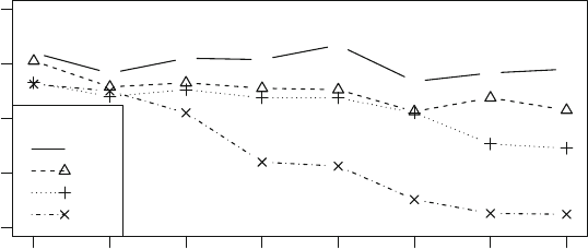
474 12 Tweedie GLMs
l
l
l
l
l
l
l
l
Time
Mean strength (kV)
1 2 4 8 16 32 48 64
0
5
10
15
20
l
Temperature
180
225
250
275
Fig. 12.8 A plot of the dialetric breakdown data (Sect. 12.4.1)
A plot of the data (Fig. 12.8) may suggest that a temperature of 275
◦
Cis
different than the rest:
> bd.means <- with(breakdown,
tapply(Strength, list(Time, Temperature), "mean"))
> matplot( bd.means, type="b", col="black",
pch=1:4, lty=1:4, las=1, ylim=c(0, 20),
xlab="Time", ylab="Mean strength (kV)", axes=FALSE)
> axis(side=1, at=1:8, labels=levels(breakdown$Time))
> axis(side=2, las=2); box()
> legend("bottomleft", pch=1:4, lty=1:4, merge=FALSE,
legend=levels(breakdown$Temperature), title="Temperature" )
The plot also seems to show that the variance increases as Time increases.
To consider fitting a Tweedie glm to the data, we use tweedie.profile()
to find an estimate of ξ:
> bd.xi <- tweedie.profile(Strength~Time*Temperature, data=breakdown,
do.plot=TRUE, xi.vec=seq(1.2, 2, length=11))
> bd.m <- glm( Strength~factor(Time) * factor(Temperature), data=breakdown,
family=tweedie(link.power=0, var.power=bd.xi$xi.max))
> anova(bd.m, test="F")
Notice that 1 <ξ<2 even though all breakdown strengths are positive:
> bd.xi$xi.max
[1] 1.591837
The Q–Q plot (Fig. 12.9, right panel) suggests no major problems with the
model:
> qqnorm( resid(bd.m), las=1 ); qqline( resid(bd.m) )

12.4 Case Studies 475
1.2 1.4 1.6 1.8 2.0
−154.5
−154.0
−153.5
−153.0
−152.5
−152.0
−151.5
−151.0
ξ index
L
l
l
l
l
l
l
l
l
l
l
l
(95% confidence interval)
l
l
l
l
l
l
l
l
l
l
l
l
l
l
l
l
l
l
l
l
l
l
ll
l
l
l
l
l
l
l
l
l
ll
l
ll
l
l
l
l
l
l
l
l
l
l
ll
l
l
l
l
l
l
l
l
ll
l
l
ll
l
l
l
l
l
l
l
l
ll
l
l
ll
l
l
l
l
l
l
l
l
ll
l
l
ll
ll
l
l
l
l
l
l
l
l
l
l
l
l
l
l
l
l
l
l
l
l
l
l
l
l
l
l
l
l
l
l
l
l
ll
−2 −1 0 1 2
−0.3
−0.2
−0.1
0.0
0.1
0.2
0.3
Normal Q−Q Plot
Theoretical Quantiles
Sample Quantiles
Fig. 12.9 The profile-likelihood plot (left panel) and Q–Q plot of quantile residuals
(right panel) for the dialetric breakdown data (Sect. 12.4.1)
1.5 2.0 2.5 3.0 3.5 4.0 4.5
46
48
50
52
54
56
ξ index
L
l
l
l
l
l
l
l
(95% confidence interval)
Fig. 12.10 The profile likelihood plot for estimating the value of the Tweedie index
parameter ξ for the poison data (Sect. 12.4.2)
12.4.2 Case Study 2
Consider the survival times data first introduced in Example 12.1, where
a Tweedie edm with ξ ≈ 4 was suggested for modelling the data (data
set: poison). To find the appropriate Tweedie edm for modelling the data
more formally, initially determine an estimate of ξ using the profile likeli-
hood (Fig. 12.10), using the r function tweedie.profile() from the package
tweedie:
> data(poison)
> library(tweedie) # To provide tweedie.profile()
476 12 Tweedie GLMs
> pn.profile <- tweedie.profile( Time ~ Trmt * Psn, data=poison,
do.plot=TRUE)
.......Done.
> c("xi: MLE"=pn.profile$xi.max, "xi: CI"=pn.profile$ci)
xi: MLE xi: CI1 xi: CI2
3.826531 2.866799 NA
These results suggest that fitting a Tweedie glm using
ˆ
ξ = 4 is not unrea-
sonable:
> library(statmod) # To provide the tweedie() family
> poison.m1 <- glm( Time ~ Trmt * Psn, data=poison,
family=tweedie(link.power=0, var.power=4))
> anova( poison.m1, test="F")
Df Deviance Resid. Df Resid. Dev F Pr(>F)
NULL 47 62.239
Trmt 3 19.620 44 42.619 32.7270 2.189e-10 ***
Psn 2 32.221 42 10.398 80.6195 5.053e-14 ***
Trmt:Psn 6 2.198 36 8.199 1.8334 0.12
---
Signif. codes: 0 '***' 0.001 '**' 0.01 '*' 0.05 '.' 0.1''1
The interaction is not significant. The fitted model without the interaction
term is:
> poison.m2 <- update( poison.m1, . ~ Trmt + Psn )
> summary(poison.m2)
Call:
glm(formula = Time ~ Trmt + Psn, family = tweedie(link.power = 0,
var.power = 4), data = poison)
Deviance Residuals:
Min 1Q Median 3Q Max
-1.29925 -0.32135 -0.03321 0.20951 0.94121
Coefficients:
Estimate Std. Error t value Pr(>|t|)
(Intercept) -0.82828 0.07938 -10.435 3.10e-13 ***
TrmtB 0.61792 0.08812 7.012 1.40e-08 ***
TrmtC 0.15104 0.06414 2.355 0.0233 *
TrmtD 0.49832 0.08053 6.188 2.13e-07 ***
PsnII -0.22622 0.09295 -2.434 0.0193 *
PsnIII -0.77091 0.08007 -9.628 3.43e-12 ***
---
Signif. codes: 0 '***' 0.001 '**' 0.01 '*' 0.05 '.' 0.1''1
(Dispersion parameter for Tweedie family taken to be 0.2656028)
Null deviance: 62.239 on 47 degrees of freedom
Residual deviance: 10.398 on 42 degrees of freedom
AIC: NA
Number of Fisher Scoring iterations: 8

12.4 Case Studies 477
l
l
IIIIII
−2
−1
0
1
2
Poison
Quantile residuals
l
ABCD
−2
−1
0
1
2
Time
Quantile residuals
l
l
l
l
l
l
l
l
l
l
l
l
l
l
l
l
l
l
l
l
l
l
l
l
l
l
l
l
l
l
l
l
l
l
l
l
l
l
l
l
l
l
l
l
l
l
l
l
0.2 0.4 0.6 0.8
−2
−1
0
1
2
Fitted values
Quantile residuals
0 10203040
0.00
0.02
0.04
0.06
0.08
0.10
0.12
Index
Cook's distance, D
l
l
l
l
l
l
l
l
l
l
l
l
l
l
l
l
l
l
l
l
l
l
l
l
l
l
l
l
l
l
l
l
l
l
l
l
l
l
l
l
l
l
l
l
l
l
l
l
−2 −1 0 1 2
−2
−1
0
1
2
Normal Q−Q Plot
Theoretical Quantiles
Sample Quantiles
Fig. 12.11 The diagnostics for the final model poison.m2 fitted to the poison data
(Sect. 12.4.2)
Notice the aic is not computed by default, because the necessary numerical
computations may be time consuming. However, the aic can be computed
explicitly using the function AICtweedie() in package tweedie, suggesting
the non-interaction model is preferred:
> c("With int" = AICtweedie(poison.m1),
"Without int." = AICtweedie(poison.m2))
With int Without int.
-87.57423 -88.32050
The diagnostic plots suggest model poison.m2 is adequate (Fig. 12.11),
though the residuals for Poison 2 are more variable than for other poisons:
> plot( qresid(poison.m2) ~ poison$Psn, las=1,
xlab="Poison", ylab="Quantile residuals" )
> plot( qresid(poison.m2) ~ poison$Trmt, las=1,
xlab="Time", ylab="Quantile residuals" )
> plot( qresid(poison.m2) ~ fitted(poison.m2), las=1,
xlab="Fitted values", ylab="Quantile residuals" )
> plot( cooks.distance(poison.m2), type="h", las=1,
ylab="Cook's distance, D")
> qqnorm( qr<-qresid(poison.m2), las=1 ); qqline(qr)
The final model is glm(Tweedie, ξ = 4; log):
y ∼ Tw
ξ=4
(ˆμ,
¯
φ =0.2656) (random)
log E[y] = log ˆμ =
ˆ
β
0
+
ˆ
β
1
x
1
+
ˆ
β
2
x
2
+
ˆ
β
3
x
3
+
ˆ
β
4
x
4
+
ˆ
β
5
x
5
(systematic)
478 12 Tweedie GLMs
where the x
j
represent dummy variables for the treatment type (j =1, 2, 3)
and poison type (j =4, 5). Observe the Pearson estimate of φ is given in the
output of summary(poisson.m2) as
¯
φ =0.2656.
These data have also been analysed [6] using the Box–Cox transformation
λ = −1, corresponding to y
∗
=1/y. This transformation is the variance-
stabilizing transformation approximating the Tweedie glm with ξ = 4 (Ta-
ble 5.2).
12.5 Using R to Fit Tweedie GLMs
Fitting Tweedie glms require extra r libraries to be installed (Sect. A.2.5):
•Thetweedie package [13] is useful for estimating the appropriate value
of ξ for a given data set using the function tweedie.profile().
•Thestatmod package [33] is essential for fitting Tweedie glms, provid-
ing the tweedie() glm family function. It also provides the function
qresid() for computing quantile residuals, whose use is strongly recom-
mended with Tweedie glms.
The tweedie.profile() function fixes the value of ξ and fits the Tweedie
glm, then computes the log-likelihood. After doing so for various values of
ξ, the profile likelihood estimate of ξ is the value producing the largest value
of the log-likelihood. The function may be slow for very large data sets.
The use of tweedie.profile() requires a formula for specifying the sys-
tematic component in the same form as used for glm(). Other important
inputs are:
• xi.vec: The vector of ξ-values to consider. By default, if the response con-
tains zeros then xi.vec = seq(1.2, 1.8, by=0.1), and if the response
does not contain zeros then xi.vec = seq(1.5, 5, by=0.5). The likeli-
hood function is smoothed by default (unless do.smooth=FALSE) through
the likelihood values computed at these values of ξ given in xi.vec.
• do.plot: Indicates whether to produce a plot of the log-likelihood against
ξ, called a profile likelihood plot. Producing the plot is recommended
to ensure the function has worked correctly and to ensure the problem
identified in Sect. 12.3.2 has not occurred. If the plot is not smooth, the
method may need to be changed. The log-likelihood is evaluated numer-
ically at the values of ξ in xi.vec, and these evaluations shown with
a filled circle in the profile likelihood plot if do.plot=TRUE (by default,
do.plot=FALSE). An interpolation spline is drawn if do.smooth=TRUE
(the default).
• method: The method used for numerically computing the log-likelihood.
Occasionally the method needs to be changed explicitly to avoid difficul-
ties (errors messages may appear; the log-likelihood may be computed as
±∞ (shown as Inf or -Inf in r); or the plot of the log-likelihood against
12.6 Summary 479
ξ is not smooth). The options include method = "series", method =
"inversion",ormethod = "interpolation". The series method [15]
often works well when the inversion method fails [16]. The interpolation
method uses either the series or an interpolation of the inversion method
results, so is often faster but may produce discontinuities in the profile
likelihood plot when the computations change regimes.
• do.ci: Produces a nominal 95% confidence interval for the mle of ξ when
do.ci=TRUE (which is the default).
The function tweedie.profile() returns numerous quantities, the most use-
ful of which are:
• xi.max: The profile likelihood estimate of ξ.
• phi.max:Themle of φ.
• ci: The limits of the approximate 95% confidence interval for ξ (returned
if do.ci=TRUE, which is the default).
See ?tweedie.profile for further information.
After installing the statmod package, specify a Tweedie glm in r us-
ing glm(formula, family=tweedie(var.power, link.power)), where the
value of ξ is var.power,andlink.power specifies the link function in the
form μ
link.power
= η. Most commonly, link.power is zero, specifying the
logarithmic link function. (The default link function is the canonical link
function; Problem 12.5.) The aic is not computed and shown in the model
summary(), because the computations may be slow. If necessary, the aic can
be computed directly using AICtweedie() in package tweedie.
12.6 Summary
Chapter 12 focuses on fitting Tweedie glms to two types of data: Tweedie
glms for positive continuous data, and Tweedie glms for positive continuous
data with exact zeros.
The Tweedie distributions are edms with the variance function V (μ)=μ
ξ
,
for ξ/∈ (0, 1) (Sect. 12.2). Special cases of Tweedie distributions previously
studied are the normal (ξ = 0), Poisson (ξ =1andφ = 1), gamma (ξ =2)
and inverse Gaussian (ξ = 3) distributions (Sect. 12.2).
The unit deviance is given in (12.2). The residual deviance D(y, ˆμ)is
suitably described by a χ
2
n−p
distribution if φ ≤ y
2−ξ
/3, but is exact when
ξ = 3 (the inverse Gaussian distribution) (Sect. 12.2.2).
For ξ ≥ 2, the Tweedie distributions, and hence Tweedie glms, are appro-
priate for positive continuous data. For 1 <ξ<2, the Tweedie distributions,
and hence Tweedie glms, are appropriate for positive continuous data with
exact zeros (Sect. 12.2).
The value of ξ is estimated using the tweedie.profile() function from
the r package tweedie (Sect. 12.3).

480 12 Tweedie GLMs
Problems
Selected solutions begin on p. 547.
12.1. Deduce the expressions for θ and κ(θ) for the Tweedie edms, as given
in (12.1)(p.460), using that V (μ)=μ
ξ
. Set the arbitrary constants of
integration to zero. (Hint: Follow the approach in Sect. 5.3.6,p.217.)
12.2. In Problem 12.1, expressions for θ and κ(θ) were found by setting the
arbitrary constants of integration to zero. In this problem we consider an
alternative parameterization [15].
1. By appropriately choosing the constants of integration, show that alter-
native expressions for θ and κ(θ) can be written as
θ =
⎧
⎪
⎪
⎨
⎪
⎪
⎩
μ
1−ξ
− 1
1 − ξ
for ξ =1
log μ for ξ =1
and κ(θ)=
⎧
⎪
⎪
⎨
⎪
⎪
⎩
μ
2−ξ
− 1
2 − ξ
for ξ =2
log μ for ξ =2
(12.6)
2. Show that θ is continuous in ξ.(Hint: Use that lim
α→0
(x
α
− 1)/α →
log x.)
3. Likewise, show that κ(θ) is continuous in ξ.
12.3. Deduce the unit deviance for the Tweedie edms given in (12.2)(p.460).
12.4. Using the guideline presented in Sect. 5.4.5 (p. 226), show that the
residual deviance D(y, ˆμ) is likely to follow a χ
2
n−p
distribution when φ ≤
y
2−ξ
/3 when ξ ≥ 1. Hence show that the saddlepoint approximation is likely
to be poor for continuous data with exact zeros.
12.5. Deduce the canonical link function for the Tweedie edms.
12.6. Consider the rescaling identity in (12.3).
1. Using this identity, deduce the Tweedie edm for which the value of φ
does not change when a change of measurement units (say, from grams
to kilograms) is applied to the data y.
2. Using this identity, deduce the Tweedie edm for which value of φ increases
by the same factor as that used for a change of measurement units in the
data y.
3. What does the identity reveal about the case of the inverse Gaussian
distribution in the case of a change in measurement units in y?
4. Show that the probability function for any Tweedie edm P
ξ
(y; μ, φ)can
be computed by an evaluation at μ = 1 (that is, P
ξ
(y
∗
;1,φ
∗
)), by finding
the appropriately-redefined values of y
∗
and φ
∗
.
12.7. Consider the Box–Cox transformation (Sect. 3.9,p.116).
12.6 Summary 481
1. Show that the Box–Cox transformation for any λ approximates fitting a
glm basedonaedm with variance function V (μ)=μ
2(1−λ)
if μ>0.
(Use a Taylor series of the transformation expanded about the mean μ,
as in Sect. 5.8.)
2. No Tweedie edms exist when 0 <ξ<1. Use this result to show no
equivalent power-variance glm exists for the Box–Cox transformations
corresponding to 0.5 <λ<1.
12.8. A study of monthly rainfall in Australia [22] fitted Tweedie glmstoa
number of different rainfall stations using
ˆ
ξ =1.6. For Bidyadanga monthly
rainfall from 1912 to 2007, the fitted systematic component was
log ˆμ
m
=2.903 + 1.908 sin(2πm/12) + 0.724 cos(2πm/12),
where m =1, 2,...12 corresponds to the month of the year (for example,
February corresponds to m = 2). The standard errors for the parameter
estimates are (respectively) 0.066, 0.090 and 0.085, and the mle of φ is 8.33.
1. Compute the Wald statistic for testing if each regression parameter is
zero.
2. Plot the value of ˆμ
m
against m for m =1,...,12 for Bidyadanga.
3. Plot the predicted value of π
0
against m for m =1,...,12 for Bidyadanga.
12.9. A study [10] of the walking habits of adults living in south-east
Queensland, Australia, compared different types of Statistical Areas classi-
fied by their walk score [9] as ‘Highly walkable’, ‘Somewhat walkable’, ‘Car-
dependent’ or ‘Very car-dependent’ (Table 12.3). The Tweedie glm was fitted
using
ˆ
ξ =1.5.
1. Explain the differences between the predicted mean walking times in
both sections of the table. Why are the predicted means all larger for the
second model (‘walking adults’)?
2. A Tweedie glm was fitted for ‘All adults’ and a gamma glm for ‘Walking
adults’. Explain why these models may have been chosen.
3. The deviance from the fitted Tweedie glm was 5976.08 on 1242 degrees
of freedom. Use this information to find an estimate of φ.
4. Using the Tweedie glm, find an estimate of the proportion of all adults
who did no walking in each of the four types of walkability descriptions,
and comment. Why are these values not the mlesoftheπ
0
?
12.10. A study of polythene use by cosmetic companies in the uk [19]
hypothesized a relationship with company turnover (Table 12.4; data set:
polythene). Consider two Tweedie glms models for the data, both using
a logarithmic link function for the systematic component: the first using
Polythene~Turnover, and the second using Polythene~log(Turnover).
1. Find estimates of ξ for each model.

482 12 Tweedie GLMs
Table 12.3 Predicted mean number of minutes of walking per day in four types of
regions, adjusted for work status, household car ownership and driver’s license status
(Problem 12.9)
All adults Walking adults
Predicted Predicted
n mean n mean
Highly walkable 214 7.5 155 25.5
Somewhat walkable 407 4.7 255 25.4
Car-dependent 441 2.9 254 21.2
Very car-dependent 187 2.5 90 18.3
Table 12.4 The company turnover and polythene use for 23 cosmetic companies in the
uk (to preserve confidentiality, the data were scaled) (Problem 12.10)
Polythene use Turnover Polythene use Turnover Polythene use Turnover
(in tonnes) (in £00 000) (in tonnes) (in £00 000) (in tonnes) (in £00 000)
0.04 0.02 31.50 9.85 587.83 83.94
1.60 0.23 472.50 21.13 1068.92 106.13
0.00 3.17 0.00 24.40 676.20 156.01
0.00 3.46 94.50 30.18 1056.30 206.43
3.78 3.55 55.94 40.13 1503.60 240.51
29.40 4.62 266.53 68.40 1438.50 240.93
8.00 5.71 252.53 70.88 2547.30 371.68
95.13 7.77 4298.70 391.33
2. Fit the glms to the data, and interpret the models.
3. On two separate plots of polythene use against turnover, plot the system-
atic components of both models, including the 95% confidence interval
for the fitted lines. Comment on the models.
4. Compute the aic for both models, and comment.
5. Produce the appropriate diagnostic plots for both models.
6. Deduce a suitable model for the data.
12.11. Consider the permeability of building material data given in Ta-
ble 11.2 (data set: perm). In Sect. 11.7 (p. 440), the positive continuous re-
sponse was modelled using an inverse Gaussian glm for interpretation rea-
sons. Jørgensen [24] also considers a gamma (ξ =2)glm for the data.
1. Determine an estimate of ξ using tweedie.profile(). What edm is
suggested?
2. Fit a suitable Tweedie glm ensuring an appropriate diagnostic analysis.
12.12. A study of human energy expenditure measured the energy expendi-
ture y of 104 females over a 24-h period (Table 12.5; data set: energy), and
also recorded their fat-tissue mass x
1
and non-fat tissue x
2
mass [18, 24].
A model for the energy expenditure is E[y]=β
1
x
1
+ β
2
x
2
, assuming the

12.6 Summary 483
Table 12.5 The energy expenditure and mass of 104 females (units not given). Only
the first six observations are shown (Problem 12.12)
Energy expenditure Mass of fat tissue Mass of non-fat tissue
60.08 17.31 43.22
60.08 34.09 43.74
63.69 33.03 48.72
64.36 9.14 50.96
65.37 30.73 48.67
66.05 20.74 65.31
.
.
.
.
.
.
.
.
.
energy expenditure for each tissue type is homogenous. Since the total mass
is M = x
1
+ x
2
, divide by M and rewrite as E[¯y]=β
2
+(β
1
− β
2
)¯x, where
¯y = y/M is the energy expenditure per unit mass, and ¯x = x
1
/M is the
proportion of fat-tissue mass.
1. Plot ¯y against ¯x and confirm the approximate linear relationship between
the variables.
2. Use tweedie.profile() to estimate ξ for the data. Which Tweedie edms
is appropriate?
3. Find a suitable glm for the data, ensuring a diagnostic analysis.
12.13. The data described in Table 12.6 (data set: motorins1) concern third
party motor insurance claims in Sweden for the year 1977 [1, 21, 32]. The
description of the data states that Swedish motor insurance companies “ap-
ply identical risk arguments to classify customers, and thus their portfolios
and their claims statistics can be combined” [1, p. 413]. The data set con-
tains 315 observations representing one of the zones in the country (covering
Stockholm, Göteborg, and Malmö with surroundings).
For the remainder of the analysis, consider payments in millions of Kroner.
Policies are categorized by kilometres of travel (five categories), the no-claim
bonus (seven categories) and make of car (nine categories), for a total of 315
categories. Of these, 20 contain exactly zero claims, so the total payout in
those categories is exactly zero; in other categories, the total payout can be
consider continuous. Find an appropriate model for the data. (Hint:You
will need to change the range of ξ values considered by tweedie.profile()
using the xi.vec input.)
Using your fitted model, interpret the model using the parameters of the
underlying Poisson and gamma distributions. (Hint: See (12.4), p. 464.)
12.14. The total monthly August rainfall for Emerald (located in Queens-
land, north eastern Australia) from 1889 to 2002 is shown in Table 12.7 (data
set: emeraldaug) with the monthly average southern oscillation index (soi).
Negative values of the soi often indicate El Niño episodes, which are often
associated with reduced rainfall in eastern and northern Australia [27].

484 12 Tweedie GLMs
Table 12.6 A description of the variables used in the Swedish insurance claims data
set (Problem 12.13)
Variable Description
Kilometres: Kilometres travelled per year:
1: Less than 1000
2: 1000–15,000
3: 15,000–20,000
4: 20,000–25,000
5: More than 25,000
Bonus: No claims bonus; the number of years since last claim, plus one
Make: 1–8 represent eight different common car models. All other models are
combined in class 9
Insured: Number of insured in policy-years
Claims: Number of claims
Payment: Total value of payments in Skr (Swedish Kroner)
Table 12.7 The total monthly rainfall in August from 1889–2002 in Emerald, Australia,
plus the monthly average soi and corresponding soi phases. The first five observations
are shown (Problem 12.14)
Year Rain (in mm) soi soi phase
1889 15.4 2.15
1890 47.5 −3.15
1891 45.7 −8.95
1892 0.0 5.92
1893 108.7 7.82
.
.
.
.
.
.
.
.
.
.
.
.
1. Argue that the Poisson–gamma models are appropriate for monthly rain-
fall data, along the lines of the argument in Sect. 12.2.4 (p. 463).
2. Perform a hypothesis test to address the relationship between rainfall and
soi given earlier in the question to see if it applies at Emerald: “Negative
values of the soi. . . are often associated with reduced rainfall in eastern
and northern Australia.”
3. Fit an appropriate edm for modelling the total monthly August rainfall
in Emerald from the soi.
4. Compute the 95% confidence interval for the soi parameter, and deter-
mine the practical importance of soi for August rainfall in Emerald.
5. Fit an appropriate edm for modelling the total monthly August rainfall
in Emerald from the soi phases.
6. Interpret the fitted model using soi phases, using the parameters of the
underlying Poisson and gamma distributions. (Hint: See (12.4), p. 464.)

12.6 Summary 485
Table 12.8 Data from 194 trawls in the South East Fisheries ecosystem regarding the
catch of tiger flathead. Distance is measured north to south on the 100 m depth contour
(Problem 12.15)
Longitude Latitude Depth Distance Swept area Number of Biomass of tiger
of trawl of trawl (in m) (in m) (in ha) tiger flathead flathead (in kg)
149.06 −37.81 −33 91 4.72260 1 0.02
149.08 −37.83 −47 90 5.00040 0 0.00
149.11 −37.87 −74 89 6.11160 153 30.70
149.22 −38.02 −117 88 5.83380 15 7.77
149.27 −38.19 −212 88 3.04222 0 0.00
150.29 −37.41 −168 48 6.11160 25 6.90
150.19 −37.33 −113 48 5.83380 53 15.30
.
.
.
.
.
.
.
.
.
.
.
.
.
.
.
.
.
.
.
.
.
12.15. A study on the South East Fisheries ecosystem near Australia [4]
collected data about the number of fish caught from fish trawl surveys. One
analysis of these data [17] studied the number of tiger flathead (Table 12.8;
data set: flathead).
1. The data record the number of flathead caught per trawl plus the to-
tal biomass of the flathead caught. Propose a mechanism for the total
biomass that leads to the Tweedie glm as a possible model (similar to
that used in Sect. 12.2.4).
2. The paper that analysed the data [17]fitsaPoissonglm to model the
number of tiger flathead caught. The paper states
...the dependence on covariates, if any, is specified using orthogonal polyno-
mials in the linear predictor. The dependency on depth used a second order
polynomial and the dependency on along-coast used a third order polyno-
mial. . . The log of the area swept variable was included as an offset (p. 542).
Explain why area is used as an offset.
3. Based on the information above, fit an appropriate Poisson glm for mod-
elling the number of tiger flathead caught (using Depth and Distance as
covariates, in the manner discussed in the quote above). Show that this
model has large overdispersion, and hence fit a quasi-Poisson model. Pro-
pose a reason why overdispersion is observed.
4. Based on the above information, plot the logarithm of biomass against
the depth and distance, and comment on the relationships.
5. The paper that analysed the biomass data [17] stated that
There is no reason to include an extra spatial dimension. . . as it would be
highly confounded with depth (p. 541).
Determine if any such correlation exists between depth, and the latitude
and longitude.

486 12 Tweedie GLMs
Table 12.9 Feeding rates (in feeds per hour) of chestnut-crowed babblers (Prob-
lem 12.16)
Feeding Observation Chick Non-breeding Brood
rate time (h) Sex age (days) birds ages size
0.000 11.09 M 1 Adult 3
0.000 11.16 M 2 Adult 4
0.000 12.81 M 3 Adult 1
0.238 12.59 M 4 Adult 1
1.316 12.16 M 5 Adult 1
1.041 11.53 M 6 Adult 1
.
.
.
.
.
.
.
.
.
.
.
.
.
.
.
.
.
.
0.321 6.22 F 19 Adult 3
0.000 6.22 M 19 Yearling 3
6. The paper that analysed the biomass data [17] used a Tweedie glm (using
Depth and Distance as covariates, in the manner discussed in the quote
above). Based on the above information, fit a suitable Tweedie glm,and
assess the model using diagnostics.
7. Compare the Q–Q plot of the deviance and quantile residuals from the
Tweedie glm, and comment.
12.16. Chestnut-crowned babblers are medium-sized Australian birds that
live in social groups. A study of their feeding habits [8] recorded, among
other things, the rates at which they fed, in feeds per hour (Table 12.9; data
set: babblers). About 18% of the feeding rates are exact zeros. Fit a Tweedie
glm to the data to model the feeding rates.
12.17. A study comparing two different types of toothbrushes [2, 30] mea-
sured the plaque index for females and males before and after brushing
(Table 12.10; data set: toothbrush). Smaller values mean cleaner teeth. The
26 subjects all used both toothbrushes. One subject received the same plaque
index before and after brushing.
Assuming the plaque index cannot become worse after brushing, fit an
appropriate glm to the data for modelling the difference (Before − After),
and deduce if the toothbrushes appear to differ in their teeth-cleaning ability,
and if this seems related to the sex of the subject.
12.18. An experiment [3] to quantify the effect of ketamine (an anaesthetic)
measured the amount of sleep (in min) for 30 guinea pigs, using five different
doses (Table 12.11; data set: gpsleep).
1. Explain what the exact zeros mean.
2. Plot the data, and show that the variance increases with the mean.
3. Plot the logarithm of the group variances against the logarithm of the
group means, where the groups are defined by the doses. Show this implies
ξ ≈ 1.

12.6 Summary 487
Table 12.10 The plaque index before and after brushing for two types of toothbrushes;
smaller values indicate cleaner teeth (Problem 12.17)
Conventional brush Hugger (new) brush
Females Males Females Males
Before After Before After Before After Before After
1.20 0.75 3.35 1.58 2.18 0.43 0.90 0.15
1.43 0.55 1.50 0.20 2.05 0.08 0.58 0.10
0.68 0.08 4.08 1.88 1.05 0.18 2.50 0.33
1.45 0.75 3.15 2.00 1.95 0.78 2.25 0.33
0.50 0.05 0.90 0.25 0.28 0.03 1.53 0.53
2.75 1.60 1.78 0.18 2.63 0.23 1.43 0.43
1.25 0.65 3.50 0.85 1.50 0.20 3.48 0.65
0.40 0.13 2.50 1.15 0.45 0.00 1.80 0.20
1.18 0.83 2.18 0.93 0.70 0.05 1.50 0.25
1.43 0.58 2.68 1.05 1.30 0.30 2.55 0.15
0.45 0.38 2.73 0.85 1.25 0.33 1.30 0.05
1.60 0.63 3.43 0.88 0.18 0.00 2.65 0.25
0.25 0.25 3.30 0.90
2.98 1.03 1.40 0.24
Table 12.11 Amount of sleep (in min) for 30 guinea pigs after receiving intravenous
dosesofketamine(Problem12.18)
0.60 mg/kg 1.04 mg/kg 1.44 mg/kg 2.00 mg/kg 2.75 mg/kg
0.00 0.00 0.00 0.00 0.00 3.60 5.59 7.67 0.00 1.71
0.00 0.00 2.85 5.92 8.32 8.50 9.40 9.77 11.15 11.89
3.99 4.78 7.36 10.43 12.73 13.20 10.92 24.80 14.48 14.75
4. Using tweedie.profile(), show that
ˆ
ξ =1.1. (Hint: Try using xi.vec
= (1.02, 1.4, by=0.02) to ensure you obtain a good estimate of ξ.)
5. Show that a quadratic Tweedie glm in Dose is significantly better than
the Tweedie glm linear is Dose.
6. Also consider the linear and quadratic Tweedie glm using log(Dose) in
place of Dose.
7. Also consider a Tweedie glm using a natural cubic spline, with knots=
quantile(Dose, c(0.33, 0.67))).
8. Plot all five systematic component on a plot of the data, and comment.
9. Use the aic to determine a model from the five considered, and show the
quadratic model in Dose is the preferred model.
488 REFERENCES
References
[1] Andrew, D.F., Herzberg, A.M.: Data: A Collection of Problems from
Many Fields for the Student and Research Worker. Springer, New York
(1985)
[2] Aoki, R., Achcar, J.A., Bolfarine, H., Singer, J.M.: Bayesian analysis
of null-intercept errors-in-variables regression for pretest/post-test data.
Journal of Applied Statistics 31(1), 3–12 (2003)
[3] Bailey, R.C., Summe, J.P., Hommer, L.D., McCracken, L.E.: A model
for the analysis of the anesthetic response. Biometrics 34(2), 223–232
(1978)
[4] Bax, N.J., Williams, A.: Habitat and fisheries production in the South
East fishery ecosystem. Final Report 1994/040, Fisheries Research and
Development Corporation (2000)
[5] Box, G.E.P.: Science and statistics. Journal of the American Statistical
Association 71, 791–799 (1976)
[6] Box, G.E.P., Cox, D.R.: An analysis of transformations (with discus-
sion). Journal of the Royal Statistical Society, Series B 26, 211–252
(1964)
[7] Brown, J.E., Dunn, P.K.: Comparisons of Tobit, linear, and Poisson-
gamma regression models: an application of time use data. Sociological
Methods & Research 40(3), 511–535 (2011)
[8] Browning, L.E., Patrick, S.C., Rollins, L.A., Griffith, S.C., Russell, A.F.:
Kin selection, not group augmentation, predicts helping in an obligate
cooperatively breeding bird. Proceedings of the Royal Society B 279,
3861–3869 (2012)
[9] Carr, L.J., Dunsiger, S.I., Marcus, B.H.: Validation of Walk Score for
estimating access to walkable amenities. British Journal of Sports
Medicine 45(14), 1144–1148 (2011)
[10] Cole, R., Dunn, P., Hunter, I., Owen, N., Sugiyama, T.: Walk score and
Australian adults’ home-based walking for transport. Health & Place
35, 60–65 (2015)
[11] Connolly, R.D., Schirmer, J., Dunn, P.K.: A daily rainfall disaggregation
model. Agricultural and Forest Meteorology 92(2), 105–117 (1998)
[12] Dunn, P.K.: Precipitation occurrence and amount can be modelled
simultaneously. International Journal of Climatology 24, 1231–1239
(2004)
[13] Dunn, P.K.: tweedie: Tweedie exponential family models (2017). URL
https://CRAN.R-project.org/package=tweedie. R package version 2.3.0
[14] Dunn, P.K., Smyth, G.K.: Randomized quantile residuals. Journal of
Computational and Graphical Statistics 5(3), 236–244 (1996)
[15] Dunn, P.K., Smyth, G.K.: Series evaluation of Tweedie exponential dis-
persion models. Statistics and Computing 15(4), 267–280 (2005)
REFERENCES 489
[16] Dunn, P.K., Smyth, G.K.: Evaluation of Tweedie exponential dispersion
models using Fourier inversion. Statistics and Computing 18(1), 73–86
(2008)
[17] Foster, S.D., Bravington, M.V.: A Poisson–gamma model for analysis of
ecological data. Environmental and Ecological Statistics 20(4), 533–552
(2013)
[18] Garby, L., Garrow, J.S., Jørgensen, B., Lammert, O., Madsen, K.,
Sørensen, P., Webster, J.: Relation between energy expenditure and body
composition in man: Specific energy expenditure in vivo of fat and fat-
free tissue. European Journal of Clinical Nutrition 42(4), 301–305 (1988)
[19] Gilchrist, R.: Regression models for data with a non-zero probability of
a zero response. Communications in Statistics—Theory and Methods
29, 1987–2003 (2000)
[20] Gilchrist, R., Drinkwater, D.: Fitting Tweedie models to data with prob-
ability of zero responses. In: H. Friedl, A. Berghold, G. Kauermann (eds.)
Statistical Modelling: Proceedings of the 14th International Workshop
on Statistical Modelling, pp. 207–214. International Workshop on Sta-
tistical Modelling, Gräz (1999)
[21] Hallin, M., François Ingenbleek, J.: The Swedish automobile portfolio in
1997. Scandinavian Actuarial Journal pp. 49–64 (1983)
[22] Hasan, M.M., Dunn, P.K.: A simple Poisson–gamma model for modelling
rainfall occurrence and amount simultaneously. Agricultural and Forest
Meteorology 150, 1319–1330 (2010)
[23] Jørgensen, B.: Exponential dispersion models (with discussion). Journal
of the Royal Statistical Society, Series B 49, 127–162 (1987)
[24] Jørgensen, B.: Exponential dispersion models and extensions: A review.
International Statistical Review 60(1), 5–20 (1992)
[25] Jørgensen, B.: The Theory of Dispersion Models. Monographs on Statis-
tics and Applied Probability. Chapman and Hall, London (1997)
[26] Jørgensen, B., de Souza, M.C.P.: Fitting Tweedie’s compound Poisson
model to insurance claims data. Scandinavian Actuarial Journal 1, 69–93
(1994)
[27] McBride, J.L., Nicholls, N.: Seasonal relationships between Australian
rainfall and the southern oscillation. Monthly Weather Review 111(10),
1998–2004 (1983)
[28] National Institute of Standards and Technology: Statistical reference
datasets (2016). URL http://www.itl.nist.gov/div898/strd
[29] Nelson, W.: Analysis of performance-degradation data from accelerated
tests. IEEE Transactions on Reliability 30(2), 149–155 (1981)
[30] Singer, J.M., Andrade, D.F.: Regression models for the analysis of
pretest/posttest data. Biometrics 53, 729–725 (1997)
490 REFERENCES
[31] Smyth, G.K.: Regression analysis of quantity data with exact zeros.
In: Proceedings of the Second Australia–Japan Workshop on Stochastic
Models in Engineering, Technology and Management, pp. 572–580. Tech-
nology Management Centre, University of Queensland, Brisbane (1996)
[32] Smyth, G.K.: Australasian data and story library (Ozdasl) (2011).
URL http://www.statsci.org/data
[33] Smyth, G.K.: statmod: Statistical Modeling (2017). URL https://
CRAN.R-project.org/package=statmod. R package version 1.4.30. With
contributions from Yifang Hu, Peter Dunn, Belinda Phipson and Yun-
shun Chen.
[34] Smyth, G.K., Jørgensen, B.: Fitting Tweedie’s compound Poisson model
to insurance claims data: Dispersion modelling. In: Proceedings of the
52nd Session of the International Statistical Institute. Helsinki, Finland
(1999). Paper Meeting 68: Statistics and Insurance
[35] Stone, R.C., Auliciems, A.: soi phase relationships with rainfall in east-
ern Australia. International Journal of Climatology 12, 625–636 (1992)
[36] Taylor, L.R.: Aggregation, variance and the mean. Nature 189, 732–735
(1961)
[37] Tweedie, M.C.K.: The regression of the sample variance on the sample
mean. Journal of the London Mathematical Society 21, 22–28 (1946)

Chapter 13
Extra Problems
Practice is the best of all instructors.
Publilius Syrus [19, Number 439]
13.1 Introduction and Overview
In previous chapters, problems were supplied relevant to the material in that
chapter. In this final chapter, we present a series of problems without the
chapter context, and often with less direction for modelling the data.
Problems
13.1. A study of pubertal timing of youths [5, Table III] tabulated the rela-
tionship between gender, when they matured, and the satisfaction with their
current weight (Table 13.1; data set: satiswt).
1. Identify the zero as either structural or sampling.
2. Find a suitable model for the data, ensuring an appropriate diagnostic
analysis.
3. Interpret the final model.
13.2. The data in Table 13.2 (data set: toxo) give the proportion of the
population testing positive to toxoplasmosis y against the annual rainfall
(in mm) x for 34 cities in El Salvador [7]. Plot the data, and describe the
important features of the data. Then, find a suitable model for the data.
(Hint: A complicated systematic component is necessary; see Problem 1.4.)
13.3. A study [15, 17] examined the effects of boric acid, a compound in
household products and pesticides, on in utero embryo damage in mice
(Table 13.3; data set: boric). Find a suitable model for modelling the ef-
fect of bromic acid on in utero damage in mice.
© Springer Science+Business Media, LLC, part of Springer Nature 2018
P. K. Dunn, G. K. Smyth, Generalized Linear Models with Examples in R,
Springer Texts in Statistics, https://doi.org/10.1007/978-1-4419-0118-7_13
491

492 13 Extra Problems
Table 13.1 The number of youths classified by gender, when they matured, and their
own opinions about their weight (Problem 13.1)
Number who wish to be
Matured Thinner Same weight Heavier
Girls Late 91 171 74
Mid 1170 861 177
Early 84 36 0
Boys Late 87 164 101
Mid 418 1300 604
Early 46 127 15
Table 13.2 The proportion of people testing positive to toxoplasmosis in 34 cities in
El Salvador (Problem 13.2)
Rainfall (in mm) Proportion Sampled Rainfall (in mm) Proportion Sampled
1735 0.50 4 1770 0.61 54
1936 0.30 10 2240 0.44 9
2000 0.20 5 1620 0.28 18
1973 0.30 10 1756 0.17 12
1750 1.00 2 1650 0.00 1
1800 0.60 5 2250 0.73 11
1750 0.25 8 1796 0.53 77
2077 0.37 19 1890 0.47 51
1920 0.50 6 1871 0.44 16
1800 0.80 10 2063 0.56 82
2050 0.29 24 2100 0.69 13
1830 0.00 1 1918 0.54 43
1650 0.50 30 1834 0.71 75
2200 0.18 22 1780 0.61 13
2000 0.00 1 1900 0.30 10
1770 0.54 11 1976 0.17 6
1920 0.00 1 2292 0.62 37
13.4. In the Birth to Ten study (btt) from the greater Johannesburg–Soweto
metropolitan area of South Africa during 1990, all mothers of singleton births
(4019 births) who had a permanent address within a defined area were inter-
viewed during a seven-week period between April and June 1990 [13]. (Sin-
gleton births are non-multiple births; that is, no twins, triplets, etc.) Five
years later, 964 of these mothers were re-interviewed.
For further research to be useful, the mothers not followed-up five years
later (Group 1) should have similar characteristics to those mothers who were
followed-up five years later (Group 2). One of the factors for comparison was
whether the mother had medical aid (similar to health insurance) at the time
of the birth of the child. Table 13.4 (data set: bttstudy) supplies these data
according to the mothers’ race.

13.1 Introduction and Overview 493
Table 13.3 The number of dead embryos D and total number of embryos T in mice at
various doses of boric acid (as percentage of feed) (Problem 13.3)
Dose 0.0 Dose 0.1 Dose 0.2 Dose 0.4
DT DT DT DT DT DT DT DT
0 15 0 8 0 6 0 13 1 12 0 10 12 12 3 12
0301311401001209 112221
1 9 2 14 1 12 1 12 0 11 1 12 0 13 3 10
112314010011013013 28311
113011214210012114 212111
213212012212014013 413111
016015014215415014 013814
011015314312014113 113015
111214010112012212 012213
2811121201216114 19811
014116313112213013 39412
013012111113010012 011212
31401411111511417 114
1 13 0 11 1 12 0 10
Table 13.4 Number of subjects whose mothers had medical aid by the race of the
participants (Problem 13.4)
White Black
Group 1 Group 2 Group 1 Group 2
Had medical aid 104 10 91 36
Had no medical aid 22 2 957 368
Total 126 12 1048 404
1. Compute the percentage of mothers in each group with medical aid.
Which group has a higher uptake of medical aid? (That is, produce a
two-way table of Group against whether or not the mother had medical
aid, combing both race categories.)
2. Compute the percentages of mothers in each group with and without
medical aid according to race. Which group has a higher uptake of medical
aid within each race? Contrast this with your answer above.
3. Explain the above paradox by fitting and interpreting the appropriate
glm for the data.
13.5. In Example 4.4, data were given regarding the time to service soft drink
vending machine routes [12]. The main interest was in predicting the amount
of time y required by the route driver to service the vending machines in
an outlet. This service activity includes stocking the machine with beverage
products and minor maintenance or housekeeping. In that example, the two
most important variables were identified as the number of cases of product
stocked x
1
and the distance walked by the route driver x
2
(Table 4.2; data
set: sdrink).

494 13 Extra Problems
Table 13.5 Canadian insurance data (Problem 13.6)
Merit Class Insured Premium Claims Cost
3 1 2,757,520 159,108 217,151 63,191
3 2 130,535 7175 14,506 4598
3 3 247,424 15,663 31,964 9589
3 4 156,871 7694 22,884 7964
3 5 64,130 3241 6560 1752
2 1 130,706 7910 13,792 4055
2 2 7233 431 1001 380
2 3 15,868 1080 2695 701
2 4 17,707 888 3054 983
2 5 4039 209 487 114
1 1 163,544 9862 19,346 5552
1 2 9726 572 1430 439
1 3 20,369 1382 3546 1011
1 4 21,089 1052 3618 1281
1 5 4869 250 613 178
0 1 273,944 17,226 37,730 11,809
0 2 21,504 1207 3421 1088
0 3 37,666 2502 7565 2383
0 4 56,730 2756 11,345 3971
0 5 8601 461 1291 382
The dependence of time on the two covariates is likely to be directly linear,
as seen in Fig. 4.1, because time should increase linearly with the number of
cases or the distance walked. Fit a suitable glm for modelling the delivery
times.
13.6. A summary of the Canadian automobile insurance industry [1] for pol-
icy years 1956 and 1957 (as of June 30, 1959) are given in Table 13.5 (data
set: cins). Virtually every insurance company operating in Canada is repre-
sented. The data are for private passenger automobile liability for non-farmers
for all of Canada apart from Saskatchewan.
The factor Merit measures the number of years since the last policy claim
(see ?cins for the details). Class is a factor based on gender, age, use and
marital status (see ?cins for the details). Insured and Premium are two mea-
sures of the risk exposure of the insurance companies. Insured is measured in
earned car-years; that is, a car insured for 6 months is 0.5 car-years. Premium
is in thousands of dollars adjusted to the premium of cars written off at 2001
rates. The data also give the number of Claims and the total Cost of the
claims in thousands of dollars.
1. Fit a glm to model the number of claims.
2. Fit a glm to model the cost per claim.
3. Fit a glm to model the total cost.
In your models, you will need to consider using an offset.

13.1 Introduction and Overview 495
Table 13.6 The number of revertant colonies for various doses of quinoline (in μgper
plate) (Problem 13.7)
Dose Colonies Dose Colonies Dose Colonies
0 15 33 16 333 33
0 21 33 26 333 38
0 29 33 33 333 41
10 16 100 27 1000 20
10 18 100 41 1000 27
10 21 100 60 1000 42
13.7. A study [2] used an Ames mutagenicity assay to count the number of
revertant colonies (colonies that revert back to the original genotype) of TA98
Salmonella in rat livers (Table 13.6; data set: mutagen). Theory [2] suggests
a good approximate model for the data is log(μ)=α + β log(d + c) − dγ for
dose d, where μ = E[Counts], γ ≥ 0, and c = 10 in this case.
1. Plot the data, using logarithm of dose on the horizontal axis.
2. Fit the suggested model to the data, and summarize. Plot this model
with the data.
3. Show that there is evidence of overdispersion.
4. Fit a negative binomial model (with the same systematic component) to
the data, and summarize.
5. Compare the two models graphically, including confidence intervals for
the fitted values.
13.8. To study the effect of trout eggs and the toxin potassium cyanate
(kscn)[9, 14], the toxin was applied at six different concentrations to vials of
fish eggs. Each vial contained between 61 and 179 eggs. The eggs in half of the
vials were allowed to water-harden for several hours after fertilization before
the kscn was applied. For the other vials, the toxin was applied immediately
after fertilization. The number of eggs in the vial after 19 days was recorded
(Table 13.7; data set: trout). Interest is in the effect of kscn concentration
on trout egg mortality.
Find an appropriate model for the proportion of eggs that do not survive,
ensuring an appropriate diagnostic analysis. Interpret the model.
13.9. In 1990, the Water Board of New South Wales, Australia, gathered
self-reported data from swimmers (Table 13.8; data set: earinf) about the
number of self-diagnosed ear infections after swimming [9, 18] to determine
if beach swimmers were more or less likely to report ear infections than non-
beach swimmers. Swimmers reported their age group (Age, with levels 15-19,
20-24 or 25-29), sex (Sex with levels Male or Female), and the number of
self-diagnosed ear infections (NumInfec), where they usually swam (Loc
, with
levels Beach or NonBeach), and whether they were a frequent ocean swimmer
(Swim, with levels Freq (frequent) or Occas (occasional)).

496 13 Extra Problems
Table 13.7 The effect on potassium cyanate concentration (in mg/L) on the mortality
of trout eggs (Problem 13.8)
Water No water Water No water
hardening hardening hardening hardening
Conc. Number Dead Number Dead Conc. Number Dead Number Dead
90 111 8 130 7 720 83 2 99 29
97 10 179 25 87 3 109 53
108 10 126 5 118 16 99 40
122 9 129 3 100 9 70 0
180 68 4 114 12 1440 140 60 100 14
109 6 149 4 114 47 127 10
109 11 121 4 103 49 132 8
118 6 105 0 110 20 113 3
360 98 6 102 4 2880 143 79 145 113
110 5 145 21 131 85 103 84
129 9 61 1 111 78 143 105
103 17 118 3 111 74 102 78
Table 13.8 The number of self-reported ear infections from swimmers (Problem 13.9)
Males Females
Frequency Usual Number Frequency Usual Number
of ocean swimming Age of of ocean swimming Age of
swimming location group infections swimming location group infections
Occasional Non-beach 15–19 0 Occasional Non-beach 15–19 0
Occasional Non-beach 15–19 0 Occasional Non-beach 15–19 0
Occasional Non-beach 15–19 0 Occasional Non-beach 15–19 4
Occasional Non-beach 15–19 0 Occasional Non-beach 15–19 10
Occasional Non-beach 15–19 0 Occasional Non-beach 20–24 0
Occasional Non-beach 15–19 0 Occasional Non-beach 20–24 0
.
.
.
.
.
.
.
.
.
.
.
.
.
.
.
.
.
.
.
.
.
.
.
.
Frequent Beach 25–29 2 Frequent Beach 25–29 2
Frequent Beach 25–29 2 Frequent Beach 25–29 2
The purpose of the study is to understand the factors that influence the
number of ear infections. Find a suitable model for the data, and interpret
this model.
13.10. A study of the root system of apple trees [6, 16] used three differ-
ent root stocks (Rstock with levels M26, Mark and MM106) and two different
spacing (Spacing, with levels 4x2 and 5x3) for eight apple trees (Plant).
Soil core samples were analysed, classified as coming from the inner or outer
zone (Zone, with levels Inner and Outer respectively) relative to each plant
(Table 13.9; data set: fineroot). The response variable is the density of fine
roots (the root length density, RLD, in cm/cm
3
); 38% of the RLD values are
zero.

13.1 Introduction and Overview 497
Table 13.9 The root length density (rld) of apple trees, rounded to two decimals
places (Problem 13.10)
M26 Mark MM106
Plant Spacing Zone rld Plant Spacing Zone rld Plant Spacing Zone rld
74× 2Outer0 1 5× 3 Inner 0 5 5 ×3Outer0
74× 2 Inner 0 1 5 ×3Outer0 5 5× 3Outer0
74× 2Outer0 1 5× 3 Inner 0 5 5 ×3Outer0
74× 2 Inner 0 1 5 ×3Outer0 5 5× 3Outer0
74× 2Outer0 1 5× 3 Inner 0 5 5 ×3 Inner 0
74× 2 Inner 0 1 5 ×3Outer0 5 5× 3Outer0
.
.
.
.
.
.
.
.
.
.
.
.
.
.
.
.
.
.
.
.
.
.
.
.
.
.
.
.
.
.
.
.
.
.
.
.
84× 2 Outer 0.42 4 4 × 2 Inner 0.30 6 5 × 3 Outer 0.48
84× 2 Inner 0.54 4 4 × 2 Inner 0.36 6 5 × 3 Outer 0.60
The design is not a full factorial design: not all plants are used with each
root stock and spacing. The Mark rootstock is used with both plant spacings,
but the other rootstocks are used at only one spacing each (M26 at 4x2,and
MM106 at 5x3).
1. Plot the data and describe the potential relationships.
2. Zone is the only variable varying within Plant, so initially fit the model
with Plant and Zone, and possibly the interaction. Find an estimate of
ξ, then fit the corresponding Tweedie glm.
3. Show that the model predicts the probability of zero rld well, but slightly
underestimates the probability for small values
4. Between plants, Rstock and Spacing vary. First, consider a Tweedie glm
with only Rstock and Zone together in the model (using the previously
estimated value of ξ). Then add Spacing, Plant and their interaction,
plus the Plant:Zone interaction to the model, and show only Rstock and
Zone and the interaction are necessary in the model.
5. Deduce a possible model for the data, ensuring a diagnostic analysis.
6. For the final model, examine the mean rld for each rootstock–zone com-
bination, and interpret.
13.11. A study of the time it takes mammals of various masses to urinate [21]
found that
mammals above 3 kg in weight empty their bladders over nearly constant duration
(p. 11,932).
In other words, the mass of the mammal is not related to urination time.
The theory presented in the paper suggests that the authors were expecting
a relationship between duration D of urination and the mass M of the form
D = kM
1/3
for some proportionality constant k (data set: urinationD).
1. By using a transformation, fit an appropriate weighted linear regression
model to all the data, and estimate the relationship between D and M.

498 13 Extra Problems
Table 13.10 The number of live births and number of Downs Syndrome births for
mothers in various age groups in British Columbia from 1961–1970 (Problem 13.12)
Mean Live Downs Synd. Mean Live Downs Synd. Mean Live Downs Synd.
age births cases age births cases age births cases
17.0 13,555 16 27.5 19,202 27 37.5 5780 17
18.5 13,675 15 28.5 17,450 14 38.5 4834 15
19.0 18,752 16 29.5 15,685 9 39.5 3961 30
20.5 22,005 22 30.5 13,954 12 40.5 2952 31
21.5 23,896 16 31.5 11,987 12 41.5 2276 33
22.5 24,667 12 32.5 10,983 18 42.4 1589 20
23.5 24,807 17 33.5 9825 13 43.5 1018 16
24.5 23,986 22 34.5 8483 11 44.5 596 22
25.5 22,860 15 35.5 7448 23 45.5 327 11
26.5 21,450 14 36.5 6628 13 47.0 249 7
2. The paper suggests that no relationship exists between D and M for
mammals heavier than 3 kg. Determine if those observation appear as
influential in the fitted model above.
3. Fit the same model as above, but to mammals heavier than 3 kg only, as
suggested by the quotation above. Are the paper’s conclusions supported?
13.12. The number of Downs Syndrome births in British Columbia, Canada,
from 1961–1970 is tabulated in Table 13.10 (data set: downs)[4, 8]. Fit an
appropriate glm to model the number of Downs Syndrome cases, and plot
the systematic component on the plot of the data. Then, fit an appropriate
glm to model the proportion of Downs Syndrome cases as a function of age.
Comment on the similarities and differences between the two models.
13.13. Blood haematology in athletes is of interest and importance at the
elite level. To this end, the Australian Institute of Sport (AIS) gathered
haematological information from 202 elite athletes across various sports [20]
(data set: AIS). The aim of the study was stated as follows:
The main aim of the statistical analysis was to determine whether there were any
hematological differences, on average, between athletes from the various sports,
between the sexes, and whether there was an effect of mass or height (p. 789).
Use the data to provide information for answering this question, focussing on
haemoglobin concentration.
13.14. A study [11] exposed 96 rainbow trout to various concentrations of 3,
4-dichloroaniline (DCA). After 28 days, the weights of the trout were recorded
(Table 13.11; data set: rtrout). The aim of the study was to “determine the
concentration level which causes 25% inhibition [i.e. weight loss] from the
control” [3, p. 161]. One analysis of the data [3] used a gamma glm with a
quadratic systematic component.

13.1 Introduction and Overview 499
Table 13.11 The weight of rainbow trout (in grams) at various doses of DCA (in μg
per litre) (Problem 13.14)
Dose of DCA (in μg per litre)
Control 19 39 71 120 210
12.7 9.4 12.7 11.9 7.7 8.8
13.3 13.9 9.2 13.2 6.4 8.7
16.3 16.4 10.4 10.5 9.8 8.6
13.8 11.8 15.3 9.5 8.8 7.3
8.7 15.0 13.3 12.5 9.9 8.6
13.6 14.3 11.1 10.4 11.1 11.4
10.6 11.0 9.4 13.1 12.1 9.9
13.8 15.0 8.2 8.4 10.5 7.3
12.5 12.2 13.2 10.6 9.0 10.6
14.7 13.3 12.1 11.3 13.7 8.4
10.9 12.3 7.9 9.6 8.4 7.4
8.9 7.0 15.3 9.1 7.6 8.3
12.7 11.3 9.6 10.6 11.0 8.5
13.0 11.8 15.5 7.4 7.8
9.1 14.6 15.3 9.6 9.7 10.1
13.7 12.4 8.2 10.3 9.5 8.2
Fit and evaluate the fitted model, suggesting another model if appropriate.
Then, using this model, estimate the dose as described in the aim.
13.15. Consider the Galápagos Islands species data (Table 13.12; data set:
galapagos)[10]. Find factors that seem to influence (a) the number of en-
demic species, and (b) the proportion of the species on each island which are
endemic. Summarize your results. Here are some hints:
• The number of species, and the proportion of endemics, are obviously
non-normal variables. You will need to choose appropriate response dis-
tributions for them.
• All of the explanatory variables are highly skew, and no regression method
could be expected to be successful without transforming them. Whenever
an explanatory variable is strictly positive and varies by a factor of 10 or
more, it is a good idea to pre-emptively apply a logarithmic transforma-
tion before undertaking any analysis. Even if the logarithmic transforma-
tion doesn’t eventually turn out to the best transformation, it will be a
big step in the right direction. For a variable like StCruz which contains
an exact zero, you could use log(StCruz+0.1), where 0.1 is the smallest
unit in which the distances are recorded.

500 REFERENCES
Table 13.12 The Galápagos Islands species data. See the help file (?galapagos)for
information on the variables (Problem 13.15)
Island
Plants
PlantEnd
Finches
FinchEnd
FinchGenera
Area
Elevation
Nearest
StCruz
Adjacent
Baltra 58 23 4 25.09 100 0.6 0.6 1.84
Bartolome 31 21 1.24 109 0.6 26.3 572.33
Caldwell 3 3 0.21 114 2.8 58.7 0.78
Champion 25 9 0.10 46 1.9 47.4 0.18
Coamano 2 1 0.05 25 1.9 1.9 903.82
Daphne Major 18 11 0.34 50 8.0 8.0 1.84
Darwin 10 7 4 2 2 2.33 168 34.1 290.2 2.85
Eden 8 4 0.03 50 0.4 0.4 17.95
Enderby 2 2 0.18 112 2.6 50.2 0.10
Espanola 97 26 3 2 2 58.27 198 1.1 88.3 0.57
Fernandina 93 35 9 0 5 634.49 1494 4.3 95.3 4669.32
Gardner (near Española) 58 17 0.57 49 1.1 93.1 58.27
Gardner (near Santa Maria) 5 4 0.78 227 4.6 62.2 0.21
Genovesa 40 19 4 3 2 17.35 76 47.4 92.2 129.49
Isabela 347 89 10 1 5 4669.32 1707 0.7 28.1 634.49
Marchena 51 23 7 1 4 129.49 343 29.1 85.9 59.56
Onslow 2 2 0.01 25 3.3 45.9 0.10
Pinta 104 37 9 2 4 59.56 777 29.1 119.6 129.49
Pinzon 108 33 9 0 5 17.95 458 10.7 10.7 0.03
Las Plazas 12 9 0.23 50 0.5 0.6 25.09
Rabida 70 30 9 0 5 4.89 367 4.4 24.4 572.33
San Cristobal 280 65 7 3 5 551.62 716 45.2 66.5 0.57
San Salvador 237 81 10 0 5 572.33 906 0.2 19.8 4.89
Santa Cruz 444 95 10 0 5 903.82 864 0.6 0.0 0.52
Santa Fe 62 28 7 1 3 24.08 259 16.5 16.5 0.52
Santa Maria 285 73 9 2 4 170.92 640 2.6 49.2 0.10
Seymour 44 16 1.84 50 0.6 9.6 25.09
Tortuga 16 8 1.24 186 6.8 50.9 17.95
Wolf 21 12 5 1 2 2.85 253 34.1 254.7 2.33
References
[1] Bailey, R.A., Simon, L.J.: Two studies in automobile insurance ratemak-
ing. ASTIN Bulletin I(IV), 192–217 (1960)
[2] Breslow, N.E.: Extra-Poisson variation in log-linear models. Applied
Statistics 33(1), 38–44 (1984)
[3] Crossland, N.O.: A method to evaluate effects of toxic chemicals on fish
growth. Chemosphere 14(11–12), 1855–1870 (1985)
[4] Davison, A.C., Hinkley, D.V.: Bootstrap Methods and their Application.
Cambridge University Press (1997)
REFERENCES 501
[5] Duncan, P.D., Ritter, P.L., Dornbusch, S.M., Gross, R.T., Carlsmith,
J.M.: The effects of pubertal timing on body image, school behavior,
and deviance. Journal of Youth and Adolescence 14(3), 227–235 (1985)
[6] Dunn, P.K., Smyth, G.K.: Series evaluation of Tweedie exponential dis-
persion models. Statistics and Computing 15(4), 267–280 (2005)
[7] Efron, B.: Double exponential families and their use in generalized linear
regression. Journal of the American Statistical Association 81(395), 709–
721 (1986)
[8] Geyer, C.J.: Constrained maximum likelihood exemplified by isotonic
convex logistic regression. Journal of the American Statistical Associa-
tion 86(415), 717–724 (1991)
[9] Hand, D.J., Daly, F., Lunn, A.D., McConway, K.Y., Ostrowski, E.: A
Handbook of Small Data Sets. Chapman and Hall, London (1996)
[10] Johnson, M.P., Raven, P.H.: Species number and endemism: The Galá-
pagos Archipelago revisited. Science 179(4076), 893–895 (1973)
[11] Maul, A.: Application of generalized linear models to the analysis of
toxicity test data. Environmental Monitoring and Assessment 23(1),
153–163 (1992)
[12] Montgomery, D.C., Peck, E.A.: Introduction to Regression Analysis. Wi-
ley, New York (1992)
[13] Morrell, C.H.: Simpson’s paradox: An example from a longitudinal study
in South Africa. Journal of Statistics Education 7 (3) (1999)
[14] O’Hara Hines, R.J., Carter, M.: Improved added variable and partial
residual plots for the detection of influential observations in generalized
linear models. Applied Statistics 42(1), 3–20 (1993)
[15] Price, J.J., Field, C.J., Field, E.A., Marr, M.C., Myers, C.B., Morrisse,
R.E., Schwetz, B.A.: Developmental toxicity of boric acid in mice and
rats. Fundamental and Applied Toxicology 18, 266–277 (1992)
[16] de Silva, H.N., Hall, A.J., Tustin, D.S., Gandar, P.W.: Analysis of dis-
tribution of root length density of apple trees on different dwarfing root-
stocks. Annals of Botany 83, 335–345 (1999)
[17] Slaton, T.L., Piergorsch, W.W., Durham, S.D.: Estimation and testing
with overdispersed proportions using the beta-logistic regression model
of Heckman and Willis. Biometrics 56(1), 125–133 (2000)
[18] Smyth, G.K.: Australasian data and story library (Ozdasl) (2011).
URL http://www.statsci.org/data
[19] Publius Syrus: The Moral Sayings of Publius Syrus, a Roman Slave: from
the Latin. L. E. Bernard & co (Translated by Darius Lyman) (1856)
[20] Telford, R.D., Cunningham, R.B.: Sex, sport, and body-size dependency
of hematology in highly trained athletes. Medicine and Science in Sports
and Exercise 23(7), 788–794 (1991)
[21] Yang, P.J., Pham, J., Choo, J., Hu, D.L.: Duration of urination does not
change with body size. Proceedings of the National Academy of Sciences
111(33), 11 932–11 937 (2014)
Appendix A
Using R for Data Analysis
The data analyst knows more than the computer.
Henderson and Velleman [7, p. 391]
A.1 Introduction and Overview
This chapter introduces the r software package. We start by discussing how
to obtain and install r and the r packages needed for this book (Sect. A.2).
We then introduce the basic use of r, including working with vectors, loading
data, and writing functions in r (Sect. A.3).
A.2 Preparing to Use R
A.2.1 Introduction to R
r is a powerful and convenient tool for fitting the models presented in this
book. Rather than a menu-driven statistical package, r is a powerful envi-
ronment for statistically and graphically analyzing data. r is free to install
and use.
While r itself is not a menu-driven package, some graphical front-ends
are available, such as r Commander [4, 5, 6](http://www.rcommander.
com/). RStudio (https://www.rstudio.com/products/RStudio/) provides an
environment for working with r which includes an integrated console, cod-
ing, graphics and help windows. R Commander is free, and free versions of
RStudio also exist.
The use of r is explained progressively throughout this book for use with
linear regression models and glms. In this appendix, some basics of using r
are described. A more comprehensive treatment of using r can be found in
the following books, among others:
© Springer Science+Business Media, LLC, part of Springer Nature 2018
P. K. Dunn, G. K. Smyth, Generalized Linear Models with Examples in R,
Springer Texts in Statistics, https://doi.org/10.1007/978-1-4419-0118-7
503
504 Appendix A
• Dalgaard [1] is a gentle introduction to using r for basic statistics.
• Maindonald and Braun [8] introduces r and covers a variety of statistical
techniques.
• Venables and Ripley [13] is an authoritative book discussing the imple-
mentation of a variety of statistical techniques in r and the closely-related
commercial program S-Plus.
A.2.2 Important R Websites
Two websites are particularly important for r users:
•Ther Project for Statistical Computing (http://www.r-project.org/)is
the r homepage. This web site contains documentation, general informa-
tion, links to searchable r mailing list archives, and much more.
• The Comprehensive r Archive Network, known as cran, contains the
files necessary for downloading r and add-on packages. A link to cran
is given from the r homepage: go to the r homepage, and select cran
from the menu. Clicking this link forces the user to select a mirror site.
(Selecting a mirror site near to you may make for faster downloads.)
Clicking on an appropriate mirror site then directs the browser to cran,
where r can be downloaded.
Another useful webpage is rseek.org, which provides a search facility dedi-
cated to r.
A.2.3 Obtaining and Installing R
r can be downloaded from cran (follow the instructions in Sect. A.2.2 to
locate cran). The procedure for then installing r depends on your operating
system (Windows; Mac OS X; linux; etc.). The easiest approach for most
users is to go to cran, then click on ‘Download and Install R’, then download
the pre-compiled binaries for your operating system. Then install these pre-
compiled binaries in the usual way for your operating system.
cran maintains current documentation for installing r. Click on the ‘Man-
uals’ link on the left (on either the cran website or the r homepage), and
read the manual R Installation and Administration. (Another manual, the
document An Introduction to R, may also prove useful for learning to use r.)
A.2.4 Downloading and Installing R Packages
Packages are collections of r functions that add extra functionality to r.
Some packages come with r, but other packages must be separately down-
loaded and installed before use. An important package used in this book
is the GLMsData package [3], which contains the data sets used in this
book. Using the r code in this book requires the GLMsData package to be
Appendix A 505
downloaded and installed, so we demonstrate the process of downloading and
installation of r packages using the GLMsData packages. More information
about the GLMsData package appears in Appendix B (p. 525).
For Windows and Mac OS X users, packages can be installed by starting
r and using the menu system:
Windows: Click Packages, then Install package(s). Select a cran mirror, then
select the package you wish to install, and then press OK.
Mac OS X: Click Packages & Data, and select CRAN (binaries) from the drop-
down menu. Clicking Get List creates a list of the packages that can be
installed from cran; make your selection, then press Update All.
Users of RStudio can install packages through the RStudio menus (under
Tools).
Alternatively, packages can be downloaded directly from cran; Sect. A.2.2
contain instructions to locate your nearest cran mirror. From the cran
homepage, select ‘Packages’, then locate and click on the name of the package
you wish to install. Here, we use the package GLMsData to demonstrate, but
the instructions are the same for downloading any r package. After clicking
on the package name in the cran list, click on the file to download for
your operating system (for example, Windows users click on the file next to
‘Windows binary’). The file will be then downloaded. To then install:
• Windows: Choose Packages from the Menu, then Install p ackage(s) from
local zip files. . . . Locate the package to install.
• Mac OS X: Click Packages & Data, select Local Binary Package, then press
Install.... Locate the package to install.
• Linux: Open a terminal and type sudo R CMD INSTALL GLMsData,for
example, in the directory where the package was downloaded, assuming
the appropriate permissions exist.
Packages can also be installed using install.packages() from the r com-
mand line; for example, install.packages("GLMsData"). Reading the doc-
ument R Installation and Administration, available at http://cran.r-project.
org/doc/manuals/R-admin.pdf, may prove useful.
A.2.5 Using R Packages
Any package, whether downloaded and installed or a package that comes
with r,mustbeloaded before being used in any r session:
• Loading: To load an installed package and so make the extra func-
tionality available to r, type (for example) library(GLMsData) (or
library("GLMsData"))atther prompt.
• Using: After loading the package, the functions in the package can be
used like any other function or data set in r.
• Obtaining help: To obtain help about the GLMsData package, even
if the package is not loaded (but is installed), type library(help=
506 Appendix A
GLMsData) (or library(help="GLMsData"))atther prompt. To ob-
tain help about particular function or data set in the package, type (for
example) ?lungcap at the r prompt after the package is loaded.
A.2.6 The R Packages Used in This Book
We have purposely kept the number of packages needed for this book to a
minimum. These packages are used in this book:
GLMsData:TheGLMsData package [3] is essential for running the r code
in this book, as it provides most of the necessary data.
MASS:TheMASS package [13] supplies the boxcox() function (Sect. 3.9),
the dose.p() function and functions used for fitting negative binomial
glms (Sect. 10.5.2). MASS comes with all r distributions, and does not
need to be downloaded and installed as described above.
splines:Thesplines package [10] is used to fit regression splines (Sect. 3.12).
splines comes with all r distributions, and does not need to be down-
loaded and installed as described above.
statmod:Thestatmod package [12] provides the tweedie() family function
used to fit Tweedie glms (Chap. 12), for computing quantile residuals
(Sect. 8.3.4), and for evaluating the probability function for the inverse
Gaussian distribution. statmod does not come with r distributions, and
must be downloaded and installed as described above.
tweedie:Thetweedie package [2] provides functions for estimating the
Tweedie index parameter ξ for fitting Tweedie glms, is used by qresid()
to compute quantile residuals for Tweedie glms, and is used for other
computations related to Tweedie glms (Chap. 12,p.457). tweedie does
not come with r distributions, and must be downloaded and installed as
described above.
The packages are loaded for use (after being downloaded and installed if
necessary) by typing
library(statmod) (for example) at the r prompt.
A.3 Introduction to Using R
A.3.1 Basic Use of R as an Advanced Calculator
After starting r, a command line is presented indicating that r is waiting for
the user to enter commands. This command line usually looks like this:
>
Instruct r to perform basic arithmetic by issuing commands at the command
line, and pressing the Enter or Return key. After starting r, enter this
command, and then press Enter (do not type the > as this is the r prompt):
>2-9*(1-3)
Appendix A 507
Note that * indicates multiplication. r responds with the answer:
[1] 20
>
After giving the answer, r then awaits your next instruction. Note that the
answer here is preceded by [1], which indicates the first item of output, and
is of little use here where the output consists of one number. Sometimes r
produces many numbers as output, when the [1] proves useful, as seen later
(Sect. A.3.5). Other examples:
>2*pi #piis3.1415...
[1] 6.283185
> -8 + ( 2^3 ) # 2^3 means 2 raised to the power 3
[1] 0
> 10/4000000 # 10 divided by a big number
[1] 2.5e-06
>1+2*3 #Note the order of operations
[1] 7
Note the use of #:the# character is a comment character, so that # and
all text after it is ignored by r. (You don’t need to type the # or the text
that follows.) The output from the final expression 2.5e-06 is r’s way of
displaying 2.5 ×10
−6
. Very large or very small numbers can be entered using
this notation also:
> 6.02e23 # Avogadro constant
[1] 6.02e+23
Standard mathematical functions are also defined in r:
> exp( 1 ) # exp(x) means e raised to the power x where e = 2.71828...
[1] 2.718282
> log( 10 ) # Notice that log is the natural log
[1] 2.302585
> log10( 10 ) # This is log to base 10
[1] 1
> log2(32) # This is log to base 2
[1] 5
> sin( pi ) # The result is zero to computer precision
[1] 1.224647e-16
> sqrt( 45 ) # The square root
[1] 6.708204
Issuing incomplete r commands forces r to wait for the command to be
completed. Suppose you wish to evaluate 2*pi*7.4, but enter this in-
complete command:
>2*pi*
508 Appendix A
r will continue to wait for you to complete the command. The prompt changes
from > to + to indicate r is waiting for further input. Continue by entering
7.4 and pressing Return. The complete interaction looks like this:
>2*pi*
+ 7.4 # DO NOT type the "+" sign: R is asking for more info
[1] 46.49557
Note that 2*piis a complete command, so if 2*piis issued at the r
prompt, r provides the answer and does not expect any further input.
A.3.2 Quitting R
To finish using r, enter the command q() at the command prompt:
> q() # This will close R
The empty parentheses are necessary. r asks if you wish to Save workspace
image? If you respond with Yes, then r will save your work, so that next time
r is started you can continue your previous r session. If you respond with
No, r starts a fresh session the next time r is started.
A.3.3 Obtaining Help in R
The following commands can be used to obtain help in r:
• help.search("glm"): search the r help system for the text glm.
• ?glm: obtain help for the function glm(); equivalent to help("glm").
• help.start(): opens r’s on-line documentation in a browser.
• RSiteSearch("generalized linear model"), if you are connected to
the Internet: Search wider r resources, such as r-help mailing list
archives, r manuals and r help pages, and displays the results in a
browser window.
• example("glm"): show an example of using glm().
A.3.4 Variable Names in R
Importantly, answers computed by r can be assigned to variables using the
two-character combination <- as shown below:
> radius <- 0.605
> area <- pi * radius^2
> area
[1] 1.149901
Appendix A 509
Notice that when <- is used, the answer is not displayed. Typing the name
of a variable shows its value. The equal sign = canbeusedinplaceof<- to
make assignments, though <- is traditional:
> radius = 0.605
Spacing in the input is not important to r. All these commands mean the
same to r, but the first is easiest to read and is recommended:
> area <- pi * radius^2
> area <- pi *radius^ 2
> area<-pi*radius^2
Variable names can consist of letters, digits, the underscore character, and
the dot (period). Variable names cannot start with digits; names starting
with dots should be avoided. Variable names are also case sensitive: HT, Ht
and ht are different variables. Many possible variables names are already in
use by r, such as log as used above. Problems may result if these are used as
variable names. Common variables names to avoid include t (for transposing
matrices), c (used for combining objects), q (for quitting r), T (is a logical
true), F (is a logical false), and data (makes data sets available to r).
These are all valid variables names: plant.height, dose2, Initial_Dose,
PatientAge,andcircuit.2.AM. In contrast, these are not valid variables
names: Before-After (the - is illegal), and 2ndTrial (starts with a digit).
A.3.5 Working with Vectors in R
r works especially well with a group of numbers, called a vector. Vectors are
created by grouping items together using the function c() (for ‘combine’ or
‘concatenate’):
> x <- c(1, 2, 3, 4, 5, 6, 7, 8, 9, 10)
> log(x)
[1] 0.0000000 0.6931472 1.0986123 1.3862944 1.6094379 1.7917595 1.9459101
[8] 2.0794415 2.1972246 2.3025851
Notice that when the output is long, r identifies the element of each list in
the left column, starting with [1]. Element 8 (which is 2.0794415) starts
the second line of output.
A long sequence of equally-spaced values is often useful, especially in plot-
ting. Rather than the cumbersome approach adopted above, consider these
simpler approaches:
> seq(0, 10, by=1) # The values are separated by distance 1
[1]012345678910
> 0:10 # Same as above
[1]012345678910
> seq(0, 10, length=9) # The result has length 9
[1] 0.00 1.25 2.50 3.75 5.00 6.25 7.50 8.75 10.00
510 Appendix A
Variables do not have to be numerical to be grouped together; text and
logical variables can be used also:
> day <- c("Sun", "Mon", "Tues", "Wed", "Thurs", "Fri", "Sat")
> hours.work <- c(0, 8, 11.5, 9.5, 8, 8, 3)
> hours.sleep <- c(8, 8, 9, 8.5, 6, 7, 8)
> do.exercise <- c(TRUE, TRUE, TRUE, FALSE, TRUE, FALSE, TRUE)
> hours.play <- 24 - hours.work - hours.sleep
> hours.awake <- hours.work + hours.play
Single or double quotes are possible for defining text variables, though double
quotes are preferred (which enables constructs like "O’Neil" and "Don’t
know").
Specific elements of a vector are identified using square brackets:
> hours.play[3]; day[ 2 ]
[1] 3.5
[1] "Mon"
As shown, commands can be issued together on one line if separated by a
; (a semi-colon). To find the value of hours.work on Fridays, consider the
following:
> day == "Fri" # A logic statement
[1] FALSE FALSE FALSE FALSE FALSE TRUE FALSE
> hours.work[ day == "Fri" ]
[1] 8
> hours.sleep[ day == "Fri" ]
[1] 7
> do.exercise[ day == "Thurs"]
[1] TRUE
Notice that == is used for logical comparisons. Other logical comparisons are
also possible:
> day[ hours.work>8] # > means "greater than"
[1] "Tues" "Wed"
> day[ hours.sleep<8] # < means "less than"
[1] "Thurs" "Fri"
> day[ hours.work >= 8 ] # >= means "greater than or equal to"
[1] "Mon" "Tues" "Wed" "Thurs" "Fri"
> day[ hours.work <= 8 ] # <= means "less than or equal to"
[1] "Sun" "Mon" "Thurs" "Fri" "Sat"
> day[ hours.work != 8 ] # != means "not equal to"
[1] "Sun" "Tues" "Wed" "Sat"
> day[ do.exercise & hours.work>8 ] # & means "and"
[1] "Tues"
> day[ hours.play>9 | hours.sleep>9 ] # | means "or"
[1] "Sun" "Thurs" "Sat"
Appendix A 511
Comparing real numbers using == should be avoided, because of the way com-
puters store floating-point numbers. (This is true for all computer languages.)
Instead, use all.equal():
> expr1 <- 0.5 - 0.3 # These two expressions should be the same
> expr2 <- 0.3 - 0.1
> c(expr1, expr2) # They *look* the same, but...
[1] 0.2 0.2
> expr1 == expr2 # ...Not exactly the same in computer arithmetic
[1] FALSE
> all.equal(expr1, expr2) # ...so use all.equal()
[1] TRUE
A.3.6 Loading Data into R
In statistics, data are usually stored in computer files, which must be loaded
into r. r requires data files to be arranged with variables in columns, and
cases in rows. Columns may have headers containing variable names; rows
may have headers containing case labels.
In r, data are usually treated as a data frame, a set of variables (nu-
meric, text, logical, or other types) grouped together. For the data entered
in Sect. A.3.5, a single data frame named my.week could be constructed:
> my.week <- data.frame(day, hours.work, hours.sleep,
do.exercise, hours.play, hours.awake)
> my.week
day hours.work hours.sleep do.exercise hours.play hours.awake
1 Sun 0.0 8.0 TRUE 16.0 16.0
2 Mon 8.0 8.0 TRUE 8.0 16.0
3 Tues 11.5 9.0 TRUE 3.5 15.0
4 Wed 9.5 8.5 FALSE 6.0 15.5
5 Thurs 8.0 6.0 TRUE 10.0 18.0
6 Fri 8.0 7.0 FALSE 9.0 17.0
7 Sat 3.0 8.0 TRUE 13.0 16.0
Entering data directly into r is only feasible for small amounts of data (and
is demonstrated, for example, in Sect. 10.4.2). Usually, other methods are
used for loading data into r:
1. If the data set comes with r, load the data using the command
data(trees) (for example), as in Example 3.14 (p. 125). Type data()
at the r prompt to see a list of all the data files that come with r.
2. If the data are in an installed r package (Sect. A.2.5), load the package,
then use data() to load the data. For example (assuming the GLMsData
is installed), load the package by typing library(GLMsData), then load
the data frame lungcap using data(lungcap) (Sect. 1.1).
512 Appendix A
3. If the data are stored as a text file (either on a storage device or on the
Internet), r provides a set of functions for loading the data:
read.csv(): Reads comma-separated text files. In files where the comma
is a decimal point and fields are separated by a semicolon, use read.
csv2().
read.delim(): Reads delimited text files, where fields are delimited by
tabs by default. In files where the comma is a decimal point, use
read.delim2().
read.table(): Reads files where the data in each line is separated by
one or more spaces, tabs, newlines or carriage returns. read.table()
has numerous options for reading delimited files.
read.fwf(): Reads data from files where the data are in a fixed width
format (that is, the data are in fields of known widths in each line of
the data file).
These functions are used by typing, for example:
> mydata <- read.csv("filename.csv")
Many other inputs are also available for these functions (see the relevant
help files). All these functions load the data into r as a data frame. These
functions can be used to load data directly from a web page (providing
you are connected to the Internet) by providing the url as the filename.
For example, the data in Table 10.20 (p. 420) are also found in tab-
delimited format at the Ozdasl webpage [11], with variable names in the
first row (called a header):
> modes <- read.delim("http://www.statsci.org/data/general/twomodes.txt",
header=TRUE)
4. For data stored in file formats from other software (such as spss, Stata,
and so on), first load the package foreign [9], then see library(help=
foreign). Not all functions in the foreign package load the data as data
frames by default (such as read.spss()).
Most data sets used in this book are available in the GLMsData package.
Assuming the GLMsData package is installed, the lungcap data frame used
in Example 1.1 (p. 1) is loaded and used as follows:
> library(GLMsData) # Loads the GLMsData package
> data(lungcap) # Makes the data set lungcap available for use
> names(lungcap) # Shows the names of the variables in lungcap
[1] "Age" "FEV" "Ht" "Gender" "Smoke"
> head(lungcap) # Shows the first six observations
Age FEV Ht Gender Smoke
1 3 1.072 46 F 0
2 4 0.839 48 F 0
3 4 1.102 48 F 0
4 4 1.389 48 F 0
5 4 1.577 49 F 0
6 4 1.418 49 F 0
Appendix A 513
> tail(lungcap) # Shows the last six observations
Age FEV Ht Gender Smoke
649 16 4.070 69.5 M 1
650 16 4.872 72.0 M 1
651 17 3.082 67.0 M 1
652 17 3.406 69.0 M 1
653 18 4.086 67.0 M 1
654 18 4.404 70.5 M 1
> str(lungcap) # Shows the structure of the data frame
'data.frame': 654 obs. of 5 variables:
$Age :int 3444444555...
$ FEV : num 1.072 0.839 1.102 1.389 1.577 ...
$ Ht : num 46 48 48 48 49 49 50 46.5 49 49 ...
$ Gender: Factor w/ 2 levels "F","M": 1111111111...
$ Smoke : int 0000000000...
A summary of the variables in a data frame is produced using summary():
> summary(lungcap) # Summaries of each variable in lungcap
Age FEV Ht Gender
Min. : 3.000 Min. :0.791 Min. :46.00 F:318
1st Qu.: 8.000 1st Qu.:1.981 1st Qu.:57.00 M:336
Median :10.000 Median :2.547 Median :61.50
Mean : 9.931 Mean :2.637 Mean :61.14
3rd Qu.:12.000 3rd Qu.:3.119 3rd Qu.:65.50
Max. :19.000 Max. :5.793 Max. :74.00
Smoke
Min. :0.00000
1st Qu.:0.00000
Median :0.00000
Mean :0.09939
3rd Qu.:0.00000
Max. :1.00000
Notice that the summary() is different for numerical and non-numerical vari-
ables.
A.3.7 Working with Data Frames in R
Data loaded from files (using read.csv() and similar functions) or using
the data() command are loaded as a data frame. A data frame is a set
of variables (numeric, text, or other types) grouped together, as previously
explained. For example, the data frame lungcap contains the data used in
Example 1.1 (p. 1). The data frame contains the variables FEV, Age, Height,
Gender and Smoke, as shown in Sect. A.3.6 in the output from the names()
command.
The data frame lungcap is visible to r, but the individual variables within
this data frame are not visible:
514 Appendix A
> library(GLMsData); data(lungcap)
> Age
Error: object "Age" not found
The objects visible to r are displayed using objects():
> objects()
[1] "lungcap"
To refer to individual variables in the data frame lungcap,use$ between the
data frame name and the variable name, as follows:
> head(lungcap$Age)
[1]344444
This construct can become tedious to use all the time. An alternative is to
use with(), by noting the data frame in which the command should executed:
> with( lungcap, head(Age) )
[1]344444
> with( lungcap, mean(Age) )
[1] 9.931193
> with( lungcap, {
c( mean(Age), sd(Age) )
})
[1] 9.931193 2.953935
> with( lungcap, {
median(Age)
IQR(Age) # Only the last is displayed
})
[1] 4
Another alternative is to attach the data frame so that the individual vari-
ables are visible to r (though this can have unintended side-effects and so
the use of attach() is not recommended):
> attach(lungcap)
> head(Age)
[1]344444
When finished using the data frame, detach it:
> detach(lungcap)
A.3.8 Using Functions in R
Working with r requires using r functions. r contains a large number of
functions, and the many additional packages add even more functions. Many
r functions have been used already, such as q(), read.table(), seq() and
Appendix A 515
log(). Input arguments to r functions are enclosed in round brackets (paren-
theses), as previously seen. All r functions must be followed by parentheses,
even if they are empty (recall the function q() for quitting r).
Many functions allow several input arguments. Inputs to r functions can
be specified as positional or named, or even both in the one call. Positional
specification means the function reads the inputs in the order in which func-
tion is defined to read them. For example, the r help for the function log()
contains this information in the Usage section:
log(x, base = exp(1))
The help file indicates that the first argument is always the number for which
the logarithm is needed, and the second (if provided) is the base for the
logarithm.
Previously, log() was called with only one input, not two. If input argu-
ments are not given, defaults are used when available. The above extract from
the help file shows that the default base for the logarithm is e ≈ 2.71828 ...
(that is, exp(1)). In contrast, there is no default value for x. This means
that if log() is called with only one input argument, the result is a natural
logarithm (since base=exp(1) is used by default). To specify a logarithm to
a different base, say base 2, a second input argument is needed:
> log(8, 2) # Same as log2(8)
[1] 3
This is an example of specifying the inputs by position. Alternatively, all or
some of the arguments can be named. For example, all these commands are
identical, computing log
2
8:
> log(x=8, base=2) # All inputs are *named*
[1] 3
> log(8, 2) # Inputs specified by position
[1] 3
> log(base=2, x=8) # Inputs named can be given in any order
[1] 3
> log(8, base=2) # Mixing positional and named inputs
[1] 3
A.3.9 Basic Statistical Functions in R
Basic statistical functions are part of r:
> library(GLMsData); data(lungcap)
> names(lungcap) # The variable names
[1] "Age" "FEV" "Ht" "Gender" "Smoke"
> length( lungcap$Age ) # The number of observations
516 Appendix A
[1] 654
> sum(lungcap$Age) / length(lungcap$Age) # The mean, the long way
[1] 9.931193
> mean( lungcap$Age ) # The mean, the short way
[1] 9.931193
> median( lungcap$Age ) # The median
[1] 10
> sd( lungcap$Age ) # The sample std deviation
[1] 2.953935
> var( lungcap$Age ) # The sample variance
[1] 8.725733
A.3.10 Basic Plotting in R
r has very rich and powerful mechanisms for producing graphics. (In fact,
there are different ways to produce graphics, including using the ggplot2
package [14].) Simple plots are easily produced, but very fine control over
many graphical parameters is possible. Consider a simple plot for the fev
data (Fig. A.1, left panel):
> data(lungcap)
> plot( lungcap$FEV ~ lungcap$Age )
The ~ command (~ is called a ‘tilde’) can be read as ‘is described by’. The
variable on the left of the tilde appears on the vertical axis. Equivalent com-
mands to the above plot() command (Fig. A.1, centre panel, p. 517)are:
> plot( FEV ~ Age, data=lungcap )
and
> with( lungcap, plot(FEV ~ Age) )
Notice the axes are labelled differently. As a general rule, r functions that
use the formula interface (that is, constructs such as FEV ~ Age) allow an
input called data, giving the data frame containing the variables.
The plot() command can also be used without using a formula interface:
> plot( lungcap$Age, lungcap$FEV )
This also produces Fig. A.1 (left panel). Using this approach, the variable
appearing as the second input is plotted on the vertical axis.
Plots can be enhanced in many ways. Compare the result of the following
code (the right panel of Fig. A.1) with the output of the previous code (the
left and centre panels of Fig. A.1):

Appendix A 517
l
l
l
l
l
l
l
l
l
l
l
l
l
l
l
l
l
l
l
l
l
l
l
l
l
l
l
l
l
l
l
l
l
l
l
l
l
l
l
l
l
l
l
l
l
l
l
l
l
l
l
l
l
l
l
l
l
l
l
l
l
l
l
l
l
l
l
l
l
l
l
l
l
l
l
l
l
l
l
l
l
l
l
l
l
l
l
l
l
l
l
l
l
l
l
l
l
l
l
l
l
l
l
l
l
l
l
l
l
l
l
l
l
l
l
l
l
l
l
l
l
l
l
l
l
l
l
l
l
l
l
l
l
l
l
l
l
l
l
l
l
l
l
l
l
l
l
l
l
l
l
l
l
l
l
l
l
l
l
l
l
l
l
l
l
l
l
l
l
l
l
l
l
l
l
l
l
l
l
l
l
l
l
l
l
l
l
l
l
l
l
l
l
l
l
l
l
l
l
l
l
l
l
l
l
l
l
l
l
l
l
l
l
l
l
l
l
l
l
l
l
l
l
l
l
l
l
l
l
l
l
l
l
l
l
l
l
l
l
l
l
l
l
l
l
l
l
l
l
l
l
l
l
l
l
l
l
l
l
l
l
l
l
l
l
l
l
l
l
l
l
l
l
l
l
l
l
l
l
l
l
l
l
l
l
l
l
l
l
l
l
l
l
l
l
l
l
l
l
l
l
l
l
l
l
l
l
l
l
l
l
l
l
l
l
l
l
l
l
l
l
l
l
l
l
l
l
l
l
l
l
l
l
l
l
l
l
l
l
l
l
l
l
l
l
l
l
l
l
l
l
l
l
l
l
l
l
l
l
l
l
l
l
l
l
l
l
l
l
l
l
l
ll
l
l
l
l
l
l
l
l
l
l
l
l
l
l
l
l
l
l
l
l
l
l
l
l
l
l
l
l
l
l
l
l
l
l
l
l
l
l
l
l
l
l
l
l
l
l
l
l
l
l
l
l
l
l
l
l
l
l
l
l
l
l
l
l
l
l
l
l
l
l
l
l
l
l
l
l
l
l
l
l
l
l
l
l
l
l
l
l
l
l
l
l
l
l
l
l
l
l
l
l
l
l
l
l
l
l
l
l
l
l
l
l
l
l
l
l
l
l
l
l
l
l
l
l
l
l
l
l
l
l
l
l
l
l
l
l
l
l
l
l
l
l
l
l
l
l
l
l
l
l
l
l
l
l
l
l
l
l
l
l
l
l
l
l
l
l
l
l
l
l
l
l
l
l
l
l
l
l
l
l
l
l
l
l
l
l
l
l
l
l
l
l
l
l
l
l
l
l
l
l
l
l
l
l
l
l
l
l
l
l
l
l
l
l
l
l
l
l
l
l
l
l
l
l
l
l
l
l
l
l
l
l
l
ll
l
l
l
l
l
l
l
l
l
l
l
l
l
l
l
l
l
l
l
l
l
l
l
l
l
l
l
l
l
l
l
l
l
l
l
l
l
l
l
l
l
l
l
l
l
51015
12345
lungcap$Age
lungcap$FEV
l
l
l
l
l
l
l
l
l
l
l
l
l
l
l
l
l
l
l
l
l
l
l
l
l
l
l
l
l
l
l
l
l
l
l
l
l
l
l
l
l
l
l
l
l
l
l
l
l
l
l
l
l
l
l
l
l
l
l
l
l
l
l
l
l
l
l
l
l
l
l
l
l
l
l
l
l
l
l
l
l
l
l
l
l
l
l
l
l
l
l
l
l
l
l
l
l
l
l
l
l
l
l
l
l
l
l
l
l
l
l
l
l
l
l
l
l
l
l
l
l
l
l
l
l
l
l
l
l
l
l
l
l
l
l
l
l
l
l
l
l
l
l
l
l
l
l
l
l
l
l
l
l
l
l
l
l
l
l
l
l
l
l
l
l
l
l
l
l
l
l
l
l
l
l
l
l
l
l
l
l
l
l
l
l
l
l
l
l
l
l
l
l
l
l
l
l
l
l
l
l
l
l
l
l
l
l
l
l
l
l
l
l
l
l
l
l
l
l
l
l
l
l
l
l
l
l
l
l
l
l
l
l
l
l
l
l
l
l
l
l
l
l
l
l
l
l
l
l
l
l
l
l
l
l
l
l
l
l
l
l
l
l
l
l
l
l
l
l
l
l
l
l
l
l
l
l
l
l
l
l
l
l
l
l
l
l
l
l
l
l
l
l
l
l
l
l
l
l
l
l
l
l
l
l
l
l
l
l
l
l
l
l
l
l
l
l
l
l
l
l
l
l
l
l
l
l
l
l
l
l
l
l
l
l
l
l
l
l
l
l
l
l
l
l
l
l
l
l
l
l
l
l
l
l
l
l
l
l
l
l
l
l
l
l
l
l
l
l
l
l
l
ll
l
l
l
l
l
l
l
l
l
l
l
l
l
l
l
l
l
l
l
l
l
l
l
l
l
l
l
l
l
l
l
l
l
l
l
l
l
l
l
l
l
l
l
l
l
l
l
l
l
l
l
l
l
l
l
l
l
l
l
l
l
l
l
l
l
l
l
l
l
l
l
l
l
l
l
l
l
l
l
l
l
l
l
l
l
l
l
l
l
l
l
l
l
l
l
l
l
l
l
l
l
l
l
l
l
l
l
l
l
l
l
l
l
l
l
l
l
l
l
l
l
l
l
l
l
l
l
l
l
l
l
l
l
l
l
l
l
l
l
l
l
l
l
l
l
l
l
l
l
l
l
l
l
l
l
l
l
l
l
l
l
l
l
l
l
l
l
l
l
l
l
l
l
l
l
l
l
l
l
l
l
l
l
l
l
l
l
l
l
l
l
l
l
l
l
l
l
l
l
l
l
l
l
l
l
l
l
l
l
l
l
l
l
l
l
l
l
l
l
l
l
l
l
l
l
l
l
l
l
l
l
l
l
ll
l
l
l
l
l
l
l
l
l
l
l
l
l
l
l
l
l
l
l
l
l
l
l
l
l
l
l
l
l
l
l
l
l
l
l
l
l
l
l
l
l
l
l
l
l
51015
1
2
34
5
Age
FEV
l
l
l
l
l
l
l
l
l
l
l
l
l
l
l
l
l
l
l
l
l
l
l
l
l
l
l
l
l
l
l
l
l
l
l
l
l
l
l
l
l
l
l
l
l
l
l
l
l
l
l
l
l
l
l
l
l
l
l
l
l
l
l
l
l
l
l
l
l
l
l
l
l
l
l
l
l
l
l
l
l
l
l
l
l
l
l
l
l
l
l
l
l
l
l
l
l
l
l
l
l
l
l
l
l
l
l
l
l
l
l
l
l
l
l
l
l
l
l
l
l
l
l
l
l
l
l
l
l
l
l
l
l
l
l
l
l
l
l
l
l
l
l
l
l
l
l
l
l
l
l
l
l
l
l
l
l
l
l
l
l
l
l
l
l
l
l
l
l
l
l
l
l
l
l
l
l
l
l
l
l
l
l
l
l
l
l
l
l
l
l
l
l
l
l
l
l
l
l
l
l
l
l
l
l
l
l
l
l
l
l
l
l
l
l
l
l
l
l
l
l
l
l
l
l
l
l
l
l
l
l
l
l
l
l
l
l
l
l
l
l
l
l
l
l
l
l
l
l
l
l
l
l
l
l
l
l
l
l
l
l
l
l
l
l
l
l
l
l
l
l
l
l
l
l
l
l
l
l
l
l
l
l
l
l
l
l
l
l
l
l
l
l
l
l
l
l
l
l
l
l
l
l
l
l
l
l
l
l
l
l
l
l
l
l
l
l
l
l
l
l
l
l
l
l
l
l
l
l
l
l
l
l
l
l
l
l
l
l
l
l
l
l
l
l
l
l
l
l
l
l
l
l
l
l
l
l
l
l
l
l
l
l
l
l
l
l
l
l
l
l
l
ll
l
l
l
l
l
l
l
l
l
l
l
l
l
l
l
l
l
l
l
l
l
l
l
l
l
l
l
l
l
l
l
l
l
l
l
l
l
l
l
l
l
l
l
l
l
l
l
l
l
l
l
l
l
l
l
l
l
l
l
l
l
l
l
l
l
l
l
l
l
l
l
l
l
l
l
l
l
l
l
l
l
l
l
l
l
l
l
l
l
l
l
l
l
l
l
l
l
l
l
l
l
l
l
l
l
l
l
l
l
l
l
l
l
l
l
l
l
l
l
l
l
l
l
l
l
l
l
l
l
l
l
l
l
l
l
l
l
l
l
l
l
l
l
l
l
l
l
l
l
l
l
l
l
l
l
l
l
l
l
l
l
l
l
l
l
l
l
l
l
l
l
l
l
l
l
l
l
l
l
l
l
l
l
l
l
l
l
l
l
l
l
l
l
l
l
l
l
l
l
l
l
l
l
l
l
l
l
l
l
l
l
l
l
l
l
l
l
l
l
l
l
l
l
l
l
l
l
l
l
l
l
l
l
ll
l
l
l
l
l
l
l
l
l
l
l
l
l
l
l
l
l
l
l
l
l
l
l
l
l
l
l
l
l
l
l
l
l
l
l
l
l
l
l
l
l
l
l
l
l
0 5 10 15 20
0
1
2
3
4
5
6
FEV vs Age
for the lungcap data
Age (years)
FEV (litres)
l
l
Females
Males
Fig. A.1 Plots of the fev data. Left panel: a simple plot; centre panel: a simple plot
produced using the data input; right panel: an enhanced plot using some of r’s graphical
parameters (Sect. A.3.10)
> plot( FEV ~ Age, # Plot FEV against Age
data=lungcap, # The data frame to use
las=1, # Ensure both axis labels are horizontal
ylim=c(0, 6), # Sets the limits of the vertical axis
xlim=c(0, 20), # Sets the limits of the horizontal axis
xlab="Age (years)", # The horizontal axis label
ylab="FEV (litres)", # The vertical axis label
main="FEV vs Age\nfor the lungcap data", # The main title
pch=ifelse(Gender=="F", 1, 19) ) # (See below)
> legend("bottomright", pch=c(1, 19), # Add legend
legend=c("Females", "Males") )
Notice that the use of \n in the main title specifies a line break.
The construct pch=ifelse(Gender=="F", 1, 19) needs explanation.
The input pch is used to select the plotting character. For example, pch=1
plots the points with an open circle, and pch=19 plots the points with a
filled circle. The complete list of plotting characters is shown by typing
example(points). Further, pch="F" (for example) would use an F as the
plotting character. The construct pch=ifelse(Gender=="F", 1, 19) is
interpreted as follows:
• For each observation, determine if Gender has the value "F" (that is, if
the gender is female). Note that the quotes are needed, otherwise r will
look for a variable named F, which is the same as the logical FALSE.Also
recall that == is used to make logical comparisons.
•IfGender does have the value "F", then use pch=1 (an open circle) to
plot the observation.
•IfGender does not have the value "F" (that is, the gender is male), then
use pch=19 (a filled circle) to plot the observation.
518 Appendix A
An alternative to using ifelse(), which would be useful if three or more
categories were to be plotted, is as follows. Begin by preparing the ‘canvas’
for plotting:
> plot( FEV ~ Age,
type="n", # Sets up the plot, but plots "n"othing
data=lungcap, las=1, ylim=c(1.5, 5),
xlab="Age (years)", ylab="FEV (litres)",
main="FEV vs Age\nfor the lungcap data")
Using type="n" sets up the canvas for plotting, but plots nothing on the plot
itself. Points are then added using points():
> points( FEV~Age, pch=1, subset=(Gender=="F"), data=lungcap )
> points( FEV~Age, pch=19, subset=(Gender=="M"), data=lungcap )
These two commands then add the points in two separate steps. The first
call to points() plots the females only (by selecting the data subset subset=
(Gender=="F")), using open circles (defined as pch=1). The second call to
points() plots the males only (subset=(Gender=="M")), using filled circles
(pch=19). Clearly, further points could be added for any number of groups
using this approach. In a similar way, lines can be added to an existing plot
using lines().
A.3.11 Writing Functions in R
One advantage of r is that functionality is easily extended by writing new
functions. Writing functions is only needed occasionally in this book.
As a simple and trivial example, consider writing a function to covert a
decimal number into a percentage:
> as.percentage <- function(x){
# Args:
# x: The decimal value to be turned into a percentage
# Returns:
# The value of x as a percentage
x * 100
}
(This r code can be typed directly into r.)
This function, called as.percentage, takes one input called x.Ther
instruction inside the brackets
{ and } shows what the function actually
does. The lines beginning with the # are comments and can be omitted, but
make the function easier to understand. This function simply multiplies the
value of x by 100. The function as.percentage canbeusedlikeanyotherr
function:
Appendix A 519
> item.cost <- c(110, 42, 25 )
> item.tax <- c( 10, 4, 2.5)
> as.percentage( item.tax / item.cost )
[1] 9.090909 9.523810 10.000000
In r functions, the value of the last unassigned expression is the value re-
turned by the function. Alternatively, the output can be assigned to a vari-
able:
> out <- as.percentage( item.tax / item.cost ); out
[1] 9.090909 9.523810 10.000000
As a more advanced example, consider adapting the function as.
percentage to return the percentage to a given number of significant figures.
In a text editor (such as Notepad in Windows; TextEdit in Mac OS X; vi or
Emacs in linux), enter:
as.percentage <- function(x, sig.figs=2){
# Args:
# x: The value to be turned into a decimal
# sig.figs: The number of significant figures
# Returns:
# The value of x as a percentage, rounded to the requested number of
# significant figures and the value with a "%" sign added at the end
percent <- signif( x * 100, sig.figs)
percent.withsymbol <- paste( percent, "%", sep="")
return( list(PC=percent, PC.symbol=percent.withsymbol ) )
}
The first line
as.percentage <- function(x, sig.figs=2){
defines the name of the function as as.percentage, and declares that it needs
two inputs: the first is called x (with no default value), and the second is called
sig.figs (with a default value of 2). The opening parenthesis
{ declares
where the instructions begin to declare what the function does; obviously,
the final closing parenthesis
} shows where the function definition ends.
The lines that follow starting with # are again comments to aid readability.
The next line computes the percentage rounded to the requested number of
significant figures:
percent <- signif( x * 100, sig.figs)
The next line adds the percentage symbol % after converting the number of
a character:
percent.withsymbol <- paste( percent, "%", sep="")
The final line is more cryptic:
return( list(PC=percent, PC.symbol=percent.withsymbol ) )
520 Appendix A
This line determines what values the function will return() when finished.
This return() command returned two values named PC and PC.withsymbol,
combined together in a list(). When the function returns an answer, one
output variable is called PC, which is assigned the value of percent,and
the second output variable is called PC.symbol, which is assigned the value
of percent.withsymbol. You can copy and paste the function into your r
session, and use it as follows:
> out <- as.percentage( item.tax / item.cost )
> out
$PC
[1] 9.1 9.5 10.0
$PC.symbol
[1] "9.1%" "9.5%" "10%"
> out <- as.percentage( item.tax / item.cost, sig.figs=3 )
> out
$PC
[1] 9.09 9.52 10.00
$PC.symbol
[1] "9.09%" "9.52%" "10%"
Functions in r can be very long and complicated (for example, including
code that detects for bad input such as trying to convert text into a percent-
age, or how to handle missing values). Writing functions are only required
in a few cases in this book, and these functions are relatively simple. For
more information on writing functions in r, see, for example, Venables and
Ripley [13] or Maindonald and Braun [8].
* A.3.12 Matrix Arithmetic in R
r performs matrix arithmetic using some special functions. A matrix is de-
fined using matrix(), where the matrix elements are given with the input
data, the number of rows with nrow or columns with ncol (or both), and op-
tionally whether to fill down columns (the default) or across rows (by setting
byrow=TRUE):
> Amat <- matrix( c(1, 2, -3, -2), ncol=2) # Fills by columns (by default)
> Amat
[,1] [,2]
[1,] 1 -3
[2,] 2 -2
> Bmat <- matrix( c(1, 5, -10, 15, -20, -25), nrow=2, byrow=TRUE) # By row
> Bmat
[,1] [,2] [,3]
[1,] 1 5 -10
[2,] 15 -20 -25
Appendix A 521
Standard matrix operations can be performed:
> dim( Amat ) # The dimensions of matrix Amat
[1]22
> dim( Bmat ) # The dimensions of matrix Bmat
[1]23
> t(Bmat) # The transpose of matrix Bmat
[,1] [,2]
[1,] 1 15
[2,] 5 -20
[3,] -10 -25
> -2 * Bmat # Multiply by scalar
[,1] [,2] [,3]
[1,] -2 -10 20
[2,] -30 40 50
Matrix multiplication of conformable matrices requires the special function
%*% to be used:
> Cmat <- Amat %*% Bmat; Cmat
[,1] [,2] [,3]
[1,] -44 65 65
[2,] -28 50 30
Multiplying non-conformable matrices produces an error:
> Bmat %*% Amat
Error in Bmat %*% Amat : non-conformable arguments
Powers of matrices are produced by repeatedly using %*%:
> Amat^2 # Each *element* of Amat is squared
[,1] [,2]
[1,] 1 9
[2,] 4 4
> Amat %*% Amat # Correct way to compute Amat squared
[,1] [,2]
[1,] -5 3
[2,] -2 -2
The usual multiplication operator * is for multiplication of scalars, not ma-
trices:
> Amat * Bmat # FAILS!!
Error in Amat * Bmat : non-conformable arrays
The * operator can also be used for multiplying the corresponding elements
of matrices of the same size:
> Bmat * Cmat
[,1] [,2] [,3]
[1,] -44 325 -650
[2,] -420 -1000 -750
522 Appendix A
The diagonal elements of matrices are extracted using diag():
> diag(Cmat)
[1] -44 50
> diag(Bmat) # diag() even works for non-square matrices
[1] 1 -20
diag() can also be used to create diagonal matrices:
> diag( c(1, -1, 2) )
[,1] [,2] [,3]
[1,]100
[2,] 0 -1 0
[3,]002
In addition, diag() can be used to create identity matrices easily:
> diag( 3 ) # Creates the 3x3 identity matrix
[,1] [,2] [,3]
[1,]100
[2,]010
[3,]001
To determine if a square matrix is singular or not, compute the determi-
nant using det():
> det(Amat)
[1] 4
> Dmat <- t(Bmat) %*% Bmat; Dmat
[,1] [,2] [,3]
[1,] 226 -295 -385
[2,] -295 425 450
[3,] -385 450 725
> det(Dmat) # Zero to computer precision
[1] -2.193801e-09
Zero determinants indicate singular matrices without inverses. (Near-zero de-
terminants indicate near-singular matrices for which inverses may be difficult
to compute.) The inverse of a non-singular matrix is found using solve():
> Amat.inv <- solve(Amat); Amat.inv
[,1] [,2]
[1,] -0.5 0.75
[2,] -0.5 0.25
> Amat.inv %*% Amat
[,1] [,2]
[1,] 1 0
[2,] 0 1
> solve(Dmat) # Not possible: Dmat is singular
Error in solve.default(Dmat) :
system is computationally singular: reciprocal
condition number = 5.0246e-18
Appendix A 523
The use of solve() to find the inverse is related to the use of solve() in
solving matrix equations of the form Ax = b where A is a square matrix,
and x unknown. For example, consider the matrix equation
1 −3
22
x
1
x
2
=
1
−3
.
In r:
> bvec <- matrix( c(1, -3), ncol=1); bvec
[,1]
[1,] 1
[2,] -3
> xvec <- solve(Amat, bvec); xvec # Amat plays the role of matrix A
[,1]
[1,] -2.75
[2,] -1.25
To check the solution:
> Amat %*% xvec
[,1]
[1,] 1
[2,] -3
This use of solve() also works if bvec is defined without using matrix().
However, the solution returned by solve() in that case is not a matrix either:
> bvec <- c(1, -3); x.vec <- solve(Amat, bvec); x.vec
[1] -2.75 -1.25
> is.matrix(x.vec) # Determines if x.vec is an R matrix
[1] FALSE
> is.vector(x.vec) # Determines if x.vec is an R vector
[1] TRUE
References
[1] Dalgaard, P.: Introductory Statistics with r, second edn. Springer Sci-
ence and Business Media, New York (2008)
[2] Dunn, P.K.: tweedie: Tweedie exponential family models (2017). URL
https://CRAN.R-project.org/package=tweedie. R package version 2.3.0
[3] Dunn, P.K., Smyth, G.K.: GLMsData: Generalized linear model data
sets (2017). URL https://CRAN.R-project.org/package=GLMsData.R
package version 1.0.0
[4] Fox, J.: The R Commander: A basic statistics graphical user interface
to R. Journal of Statistical Software 14(9), 1–42 (2005)
524 Appendix A
[5] Fox, J.: Using the R Commander: A Point-and-Click Interface for R.
Chapman and Hall/CRC Press, Boca Raton FL (2017)
[6] Fox, J., Bouchet-Valat, M.: Rcmdr: R Commander (2016). URL http://
socserv.socsci.mcmaster.ca/jfox/Misc/Rcmdr/. R package version 2.3.1
[7] Henderson, H.V., Velleman, P.F.: Building multiple regression models
interactively. Biometrics 37(2), 391–411 (1981)
[8] Maindonald, J.H., Braun, J.: Data Analysis and Graphics using R, third
edn. Cambridge University Press, UK (2010)
[9] R Core Team: foreign: Read Data Stored by Minitab, S, SAS, SPSS,
Stata, Systat, Weka, dBase, ... (2017). URL https://CRAN.R-project.
org/package=foreign. R package version 0.8-69
[10] R Core Team: R: A Language and Environment for Statistical Comput-
ing. R Foundation for Statistical Computing, Vienna, Austria (2017).
URL https://www.R-project.org/
[11] Smyth, G.K.: Australasian data and story library (Ozdasl) (2011). URL
http://www.statsci.org/data
[12] Smyth, G.K.: statmod: Statistical Modeling (2017). URL https://
CRAN.R-project.org/package=statmod. R package version 1.4.30. With
contributions from Yifang Hu, Peter Dunn, Belinda Phipson and Yun-
shun Chen.
[13] Venables, W.N., Ripley, B.D.: Modern Applied Statistics with S, fourth
edn. Springer-Verlag, New York (2002)
[14] Wickham, H.: ggplot2: Elegant Graphics for Data Analysis. Springer-
Verlag New York (2009)
Appendix B
The GLMsData package
If you have only pretend data, you can only pretend to
analyze it.
Watkins, Scheaffer and Cobb [2,p.x]
Almost all of the data files used in this book are collated in the r package
GLMsData [1]. This package is available from cran, and is downloaded and
installed like any other r package (Sect. A.2.5). The version of GLMsData
used to prepare this book is 1.0.0. Since the publication of this book, the
contents of the GLMsData package may have been updated.
A list of the 97 data files in the GLMsData package appear below, with
a brief description. For more details about the GLMsData package in gen-
eral, enter library(help = "GLMsData") at the r prompt, assuming the
GLMsData package is installed. For more information about any individ-
ual data set, say lungcap,enter?lungcap at the r prompt (assuming the
GLMsData package is installed and loaded).
AIS Australian Institute of Sports (AIS) data
ants Ants species richness
apprentice Apprentice migration to Edinburgh
babblers Feeding rates of babblers
belection British election candidates
blocks Blocks stacked by children
boric Dead embryos after exposure to boric acid
breakdown Dialetric breakdown data
bttstudy The South African Birth to Ten (BTT) study
budworm Insecticide doses and tobacco budworm
butterfat Butterfat and dairy cattle
ccancer Canadian cancers
ceo CEO salaries
cervical Deaths from cervical cancer
cheese Tasting cheese
cins Canadian car insurance data
crawl The age at which babies start to crawl
cyclones Cyclones near Australia
danishlc Danish lung cancer
dental Decayed, missing and filled teeth
deposit Insecticides
downs Downs Syndrome cases in British Columbia
© Springer Science+Business Media, LLC, part of Springer Nature 2018
P. K. Dunn, G. K. Smyth, Generalized Linear Models with Examples in R,
Springer Texts in Statistics, https://doi.org/10.1007/978-1-4419-0118-7
525
526 Appendix B
dwomen Depression and children
dyouth Depression in adolescents
earinf Ear infections in swimmers
emeraldaug August monthly rainfall in Emerald
energy Energy expenditure
failures Failures of electronic equipment
feedrates Feeding rates of birds
fineroot The root length density of apple trees
fishfood Food consumption for fish
flathead Tiger flathead from trawls
flowers The average number of meadowfoam flowers
fluoro The time of fluoroscopy and total radiation
galapagos Gal\'apagos Island species data
germ Germination of seeds
germBin Germination of seeds
gestation Gestation time
gforces G-induced loss of consciousness
gopher Clutch sizes of Gopher tortoises
gpsleep Sleep times for guinea pigs
grazing Bird abundance in grazing areas
hcrabs Males attached to female horseshoe crabs
heatcap Heat capacity of hydrobromic acid
humanfat Human age and fatness
janka Janka hardness
kstones Treating kidney stones
lactation Lactation of dairy cows
leafblotch Percentage leaf area of leaf blotch
leukwbc Leukaemia survival times
lime Small-leaved lime trees
lungcap Lung capacity and smoking in youth
mammary Adult mammary stem cells
mandible Mandible length and gestational age
manuka Manuka honey and wound healing
motorins Swedish third-party car insurance
mutagen Mutagenicity assay
mutantfreq Cell mutant frequencies in children
nambeware Nambeware products
nhospital Naval hospital maintenance
nitrogen Soil nitrogen
nminer Noisy miner abundance
paper The tensile strength of paper
perm Permeability of building materials
phosphorus Soil phosphorus
pock Pock counts
poison Survival times of animals
polyps The number of polyps and suldinac
polythene Cosmetic company use of polythene
punting Football punting
quilpie Total July rainfall at Quilpie
ratliver Drugs present in rat livers
rootstock Rootstock data
rrates Oxidation rate of benzene
rtrout Weights of rainbow trout
ruminant Energy in ruminant's diets
Appendix B 527
satiswt Satisfaction with weight in youth
sdrink Soft drink delivery times
seabirds Counts of seabirds
serum Mice surviving doses of antipneumococcus serum
setting Heat evolved by setting cement
sharpener Sharpener data
sheep The daily energy requirements for wethers
shuttles O-rings on the space shuttles
teenconcerns Concerns of teenagers
toothbrush Effectiveness of toothbrushes
toxo Toxoplasmosis and rainfall
triangle Artificial data from triangles
trout The effect of potassium cyanate on trout eggs
turbines Fissures in turbine wheels
urinationD Urination time
urinationL Urethral length
wacancer Cancer in Western Australia
wheatrain Annual rainfall in the NSW wheat belt
windmill Power generation by windmills
wwomen Smoking and survival
yieldden Yield of onions at various densities
References
[1] Dunn, P.K., Smyth, G.K.: GLMsData: Generalized linear model data sets
(2017). URL https://CRAN.R-project.org/package=GLMsData. R pack-
age version 1.0.0
[2] Watkins, A.E., Sheaffer, R.L., Cobb, G.W.: Statistics in Action, second
edn. Key Curriculum Press (2008)
Selected Solutions
Research has shown that it is effective to combine
example study and problem solving in the initial
acquisition of cognitive skills.
Renkl [3, p. 293]
The data used generally come from the GLMsData [2] package. We do not
explicitly load this package each time it is needed.
> library(GLMsData)
Solutions to Problems from Chap. 1
1.1 The more complex quartic model is similar to the cubic. The cubic is possibly
superior to the quadratic, so we probably prefer the cubic.
1.4 The proportion testing positive is between zero and one. The cubic regression
model is not good—it permits proportions outside the physical range; the cubic glm is
preferred.
1.5 1. Linear in the parameters; suitable for linear regression and glms. 2. Not linear in
parameters. 3. Linear in the parameters; suitable for glms. 4. Linear in the parameters;
suitable for glms.
1.6
> data(turbines)
> ### Part 1
> names(turbines)
> ### Part 4
> summary(turbines)
> ### Part 5
> plot(Fissures/Turbines ~ Hours, data=turbines, las=1)
2. All variables are quantitative. 3. Clearly the number of hours run is important for
knowing the proportion of fissures. The proportion must be between 0 and 1 obviously.
1.9
> data(blocks); blocks$Trial <- factor(blocks$Trial)
> blocks$cutAge <- cut(blocks$Age, breaks=c(0, median(blocks$Age), Inf))
> ### Part 1
© Springer Science+Business Media, LLC, part of Springer Nature 2018
P. K. Dunn, G. K. Smyth, Generalized Linear Models with Examples in R,
Springer Texts in Statistics, https://doi.org/10.1007/978-1-4419-0118-7
529

530 Selected Solutions
> summary(blocks)
> ### Part 2
> par( mfrow=c(2, 4))
> plot( Time~Shape, data=blocks, las=1)
> plot( Time~Trial, data=blocks, las=1)
> plot( Time~Age, data=blocks, las=1)
> with(blocks, interaction.plot(Shape, cutAge, Time))
> ### Part 4
> plot( Number~Shape, data=blocks, las=1)
> plot( Number~Trial, data=blocks, las=1)
> plot( Number~Age, data=blocks, las=1)
> with(blocks, interaction.plot(Shape, cutAge, Number))
3. For both responses: shape seems important; trial number doesn’t; age possibly. 5. Per-
haps interactions.
Solutions to Problems from Chap. 2
2.1 1. β
0
is the predicted value when x =0.2. α
0
is the predicted value when x is
equal to the mean of x (that is,
x). The second form may allow a better interpretation
of the constant, since x = 0 may be far from the values of x used to fit the model.
2.2 Solve the equations. Note that
w
i
(x
i
− ¯x
w
)
2
=
w
i
x
2
i
−
w
i
x
i
2
/
w
i
.
and
w
i
(x
i
−¯x
w
)y
i
=
w
i
x
i
y
i
−
w
i
x
i
¯y
w
, which makes the connection to the given
formula a bit easier to see.
2.4 1. Expand S =(y − Xβ)
T
W(y − Xβ) to get the result. 2. Differentiating with
respect to β gives ∂S/∂β = −2X
T
Wy +2X
T
WXβ. 3. Setting the differential to zero
and solving gives X
T
Wy
T
=X
T
WXβ. Pre-multiplying by (X
T
WX)
−1
gives the result.
2.6 E[
ˆ
β]=(X
T
WX)
−1
X
T
WE[y]=(X
T
WX)
−1
X
T
W(Xβ)=β.
2.8 Substituting for R
2
on the right in terms of ss gives {ssReg/(p
−1)}/{sst/(n−p
)},
which is F .
2.9 1. A:
11111
11−1 −10
T
;B:
11111
111−1 −1
T
;C:
1111 1
10.50−0.5 −1
T
.
2. Then, use that var[ˆμ]=x
g
(X
T
X)
−1
x
T
g
with x
g
=[1 x] to obtain var[ˆμ
A
]=(1/4)
+x
2
/5; var[ˆμ
B
]=(5− 6x +5x
2
)/16; var[ˆμ
B
]=(1− 2x
2
)/5.
> x <- seq(-1, 1, length=100)
> xA <- c(1, 1, -1, -1, 0)
> xB <- c(1, 1, 1, 1, -1)
> xC <- c(1, 0.5, 0, -0.5, -1)
> varA <- function(x){0.25 + x^2/5}
> varB <- function(x){(5 - 6*x + 5*x^2)/16}
> varC <- function(x){(1+2*x^2)/5}
> vA <- varA(x); vB <- varB(x); vC <- varC(x)
> plot( range(c(vA, vB, vC)) ~ range(x), type="n", ylim=c(0, 1.2),
ylab="Var. of predictions", xlab="x values", las=1)
> lines(varA(x) ~ x, lty=1, lwd=2)
> lines(varB(x) ~ x, lty=2, lwd=2)
Selected Solutions 531
> lines(varC(x) ~ x, lty=3, lwd=2)
> legend("top", lwd=2, lty=1:3, legend=c("Design A", "Design B",
"Design C"))
As would be expected from the location of the x values: A produces the most uni-
form small prediction errors; B produces smaller prediction errors for larger x values; C
produces smaller prediction errors in the middle of the range of x values.
2.10 1. The Taylor series expansion is f(x)=f(¯x)+df/dx(x−¯x)+d
2
f/dx
2
(x−¯x)
2
/2+
···. 2. f(x) is linear in x,ifx − ¯x is small. 3. Any function can be considered locally
approximately linear.
2.15 2. The relationship between the number of flowers per plant and light intensity
has different intercepts for the different timings, but the same slope. 3. The relationship
between the number of flowers per plant and light intensity has different intercepts and
different slopes for the different timings. 4. Interaction term doesn’t seem necessary.
5. Makes no difference to the parameter estimates or standard errors. However, the
estimate of σ is different. 6. The interaction term does not seem needed.
> data(flowers)
> wts <- rep(10, length(flowers$Light) )
> ### Part 1
> plot(Flowers~Light, data=flowers, pch=ifelse(Timing=="PFI", 1, 19))
> legend("topright", pch=c(1, 19), legend=c("PFI","Before PFI"))
> ### Part 3
> m1 <- lm(Flowers~Light*Timing, data=flowers, weights=wts); anova(m1)
> m2 <- lm(Flowers~Light+Timing, data=flowers, weights=wts); anova(m2)
> ### Part 5
> m1.nw <- lm(Flowers~Light*Timing, data=flowers); anova(m1.nw)
> m2.nw <- lm(Flowers~Light+Timing, data=flowers); anova(m2.nw)
> summary(m1); summary(m1.nw)
> ### Part 6
> abline(coef(m2)[1], coef(m2)[2], lty=1)
> abline(sum(coef(m2)[c(1, 3)]), coef(m2)[2], lty=2)
2.18
> data(blocks)
> ### Part 5
> m0 <- lm( Time ~ Shape, data=blocks); anova( m0 )
> mA <- lm( Time ~ Trial + Age + Shape, data=blocks); anova( mA )
> ### Part 6
> mB <- update(mA, . ~ Trial + Age*Shape); anova( mB )
> t.test(Time~Shape, data=blocks)
> summary(m0)
> ### Part 7
> m1 <- lm( Time~Shape, data=blocks); anova(m1)
1. Possible increasing variance. Perhaps non-linear? 2. The relationship between age
and time has different intercepts and slopes for the two shapes. 3. Time depends on age
and trial number, and the effect of age depends on the trial number. 4. Time depends
on age and shape, and both depend on the trial number. 8. On average, the time taken
to stack cylinders is 14.45slessthanforcubes.
532 Selected Solutions
Solutions to Problems from Chap. 3
3.2 Expand the expressions, simplify, and the results follow.
3.8
> data(lungcap)
> ### Part 1
> m1 <- lm(FEV~factor(Smoke), data=lungcap)
> ### Part 2
> m2 <- lm(FEV~factor(Smoke)+Age+Ht+factor(Gender), data=lungcap)
> ### Part 3
> m3 <- lm(log(FEV)~factor(Smoke)+Age+Ht+factor(Gender), data=lungcap)
> ### Part 4
> summary(m1); summary(m2); summary(m3); anova(m3) # Prefer m3
1. Smokers have a larger fev by an average of 0.7107 L. 2. Smokers have a smaller fev
by an average of −0.08725 L. 3. Smokers have a smaller fev by, on average, a factor of
0.9165.
3.10
> data(cheese)
> m4 <- lm( log(Taste) ~ log(H2S) + Lactic + Acetic, data=cheese )
> scatter.smooth( rstandard(m4) ~ fitted(m4) )
> qqnorm( rstandard(m4) ); qqline( rstandard(m4) )
> plot( cooks.distance(m4), type="h")
3.11
> data(fishfood); par(mfrow=c(2, 3))
> ### Part 1
> m1 <- lm( log(FoodCon) ~ log(MaxWt) + log(Temp) + log(AR) + Food,
data=fishfood); anova(m1)
> ### Part 2
> plot(rstandard(m1)~fitted(m1)); qqnorm(rstandard(m1))
> plot( cooks.distance(m1), type="h") # Model looks OK
> m2 <- update(m1, . ~ log(MaxWt) * log(Temp) * Food * log(AR))
> m3 <- step(m2); anova(m1, m3) # Model m3 a bit better
> plot(rstandard(m3)~fitted(m3)); qqnorm(rstandard(m3))
> plot( cooks.distance(m3), type="h") # Model looks OK
3. Unravelling, the model has the form ˆμ =exp(β
0
)x
β
1
1
x
β
2
2
···. 4. The interaction model
is slightly better if the automated procedure can be trusted, by the ANOVA test (and
AIC).
3.13
> data(flowers)
> m1 <- lm(Flowers~Light+Timing, data=flowers)
> ### Part 1
> scatter.smooth( rstandard(m1) ~ fitted(m1) )
> qqnorm( rstandard(m1) ); qqline( rstandard(m1) )
> plot( cooks.distance(m1), type="h")
> plot( rstandard(m1) ~ flowers$Light)
> ### Part 2
> rowSums(influence.measures(m1)$is.inf)
Selected Solutions 533
2. No observations reported as influential.
3.16
> data(blocks); par(mfrow=c(2, 4))
> m1 <- lm( Time~Shape, data=blocks); anova(m1)
> ### Part 1
> plot( rstandard(m1) ~ fitted(m1) )
> qqnorm( rstandard(m1) ); qqline( rstandard(m1) )
> plot( cooks.distance(m1), type="h")
> plot( rstandard(m1) ~ blocks$Shape)
> rowSums(influence.measures(m1)$is.inf)
> ### Part 2
> m2 <- lm( log(Time)~Shape*Age, data=blocks); anova(m2)
> m2 <- update(m2, .~Shape+Age); anova(m2)
> m2 <- update(m2, .~Shape); anova(m2)
> plot( rstandard(m2) ~ fitted(m2) )
> qqnorm( rstandard(m2) ); qqline( rstandard(m2) )
> plot( cooks.distance(m2), type="h")
> plot( rstandard(m2) ~ blocks$Shape)
> rowSums(influence.measures(m2)$is.inf)
1. The model includes only Shape. The Q–Q plot shows non-normality; the variance is
different between cubes and cylinders. Perhaps influential observations. 2. The model
diagnostics appear better, if not perfect, after applying a log-transform.
3.21
> data(paper)
> ### Part 1
> plot( Strength~Hardwood, data=paper)
> ### Part 2
> m1 <- lm(Strength ~ poly(Hardwood, 5), data=paper); summary(m1)
> ### Part 3
> m2 <- lm(Strength ~ ns(Hardwood, df=7), data=paper); summary(m2)
> ### Part 4
> newH <- seq( min(paper$Hardwood), max(paper$Hardwood), length=100)
> newy1 <- predict( m1, newdata=data.frame(Hardwood=newH))
> newy2 <- predict( m2, newdata=data.frame(Hardwood=newH))
> lines(newy1~newH)
> lines(newy2~newH, lty=2)
3.23
> data(gopher)
> ### Part 1
> par( mfrow=c(2, 2))
> plot( ClutchSize ~ Temp, data=gopher)
> plot( ClutchSize ~ Evap, data=gopher)
> ### Part 3
> gt.lm <- lm( ClutchSize ~ Temp + Evap, weights=SampleSize, data=gopher)
> summary(gt.lm)
> ### Part 4
> anova(gt.lm)
> ### Part 5
> cor(cbind(gopher$ClutchSize, gopher$Temp, gopher$Evap, gopher$Latitude))

534 Selected Solutions
> ### Part 6
> plot( Evap ~ Latitude, data=gopher)
> plot( Temp ~ Latitude, data=gopher)
> m1 <- lm(ClutchSize~Evap, data=gopher)
> par(mfrow=c(2, 2))
> plot( rstandard(m1) ~ gopher$Latitude)
> plot( rstandard(m1) ~ fitted(m1))
> plot(cooks.distance(m1), type="h")
> qqnorm( rstandard(m1)); qqline( rstandard(m1))
1. Some reasonable positive relationships. 2. Each site has a different number of
clutches. 3. No significant explanatory variables. 4. No significant explanatory variables.
6. Evaporation and temperature look related to latitude.
3.25
> data(ratliver)
> ### Part 1
> plot( DoseInLiver ~ BodyWt, data=ratliver)
> plot( DoseInLiver ~ LiverWt, data=ratliver)
> plot( DoseInLiver ~ Dose, data=ratliver)
> ### Part 2
> m1 <- lm(DoseInLiver ~ BodyWt + LiverWt + Dose, data=ratliver)
> ### Part 3
> summary(m1); anova(m1)
> ### Part 4
> influence.measures(m1)
> infl <- which.max(cooks.distance(m1))
> ### Plot 5
> plot(BodyWt ~ Dose, data=ratliver)
> points(BodyWt ~ Dose, subset=(infl), pch=19, data=ratliver)
> ### Plot 6
> m2 <- update(m1, subset=(-infl) ); summary(m2); anova(m2)
1. Possible relationships.
Solutions to Problems from Chap. 4
4.2 Apply the derivatives and the results follow.
4.5
1. For one observation: = −log μ − y/μ.
2. U(μ)=−n/μ +
y
i
/μ
2
= n(ˆμ −μ)/μ
2
.
3. ˆμ =
y
i
/n.
4. J(μ)=(−nμ +2
y
i
)/μ
3
= −n(μ − 2ˆμ)/μ
3
; I(μ)=n/μ
2
.
5. se(ˆμ)=I(ˆμ)
−1/2
= μ/
√
n.
6. W = n(ˆμ − 1)
2
/ˆμ
2
.
7. S = n(ˆμ − 1)
2
.
8. L =2n(ˆμ − log ˆμ − 1).
10. W, S and L are similar near ˆμ, but dissimilar far away from ˆμ. For larger values of
n, the curves are sharper at ˆμ, so there is more information.
Selected Solutions 535
> par(mfrow=c(1, 2))
> muhat <- seq(0.5, 2, length=200)
> ### Part 9
>n<-10
> W <- (muhat-1)^2/(muhat^2/n)
> S <- n*(muhat-1)^2
> L <- 2*n*(muhat-log(muhat)-1)
> plot(range(W)~range(muhat), type="n", main="n = 10", xlab="x", ylab="")
> lines(W~muhat)
> lines(S~muhat, lty=2)
> lines(L~muhat, lty=3)
> legend("top", lty=1:3, legend=c("Wald","Score","LRT"))
> abline(v=1, lty=4)
> ### Part 10
>n<-100
> W <- (muhat-1)^2/(muhat^2/n)
> S <- n*(muhat-1)^2
> L <- 2*n*(muhat-log(muhat)-1)
> plot(range(W)~range(muhat), type="n", main="n = 100", xlab="x", ylab="")
> lines(W~muhat)
> lines(S~muhat, lty=2)
> lines(L~muhat, lty=3)
> legend("top", lty=1:3, legend=c("Wald","Score","LRT"))
> abline(v=1, lty=4)
4.6
> set.seed(252627)
> n <- 200; yy <- rexp(n, 1); len.mu <- 250
> #Part 1:
> muhat.vec <- seq(0.75, 1.25, length=len.mu)
> llh <- array(dim=len.mu)
> for (i in (1:length(muhat.vec))){
llh[i] <- sum( log( dexp(yy, rate=1/muhat.vec[i]) ) )
}
> plot(llh~muhat.vec, type="l", lwd=2, las=1, xlab="mu")
> muhat <- mean(yy); critical <- qchisq(1-0.05, df=1)
> abline(v=1); abline(v=muhat); abline(h=max(llh)- critical, lty=2)
> # Part 2:
> W <- (muhat-1)^2/(muhat^2/n); S <- n * (muhat-1)^2
> L <- 2*n*(muhat - log(muhat)-1)
> c(W, S, L); pexp( c(W, S, L), rate=1, lower.tail=FALSE)
> # Part 3:
> W <- (muhat.vec-1)^2/(muhat.vec^2/n); S <- n * (muhat.vec-1)^2
> L <- 2*n*(muhat.vec - log(muhat.vec)-1)
> plot(W~muhat.vec, type="l", lwd=2, ylab="Test statistic", xlab="mu hat")
> lines(S~muhat.vec, lty=2, lwd=2); lines(L~muhat.vec, lty=3, lwd=2)
> abline(v=1); abline(v=muhat); abline(h=critical)
> legend("top", lty=1:3, legend=c("Wald","Score","L. Ratio"),
lwd=2, bg="white")
> # Parts 4 and 5
> se <- sqrt(muhat/n); se; c(muhat - se*1.960, muhat+se*1.960)

536 Selected Solutions
Solutions to Problems from Chap. 5
5.1 2. Geometric: θ =log(1− p); κ(θ)=log{(1 −p)/p}; φ =1.5. Strict arcsine:
θ =logp; κ(θ)=arcsinp; φ =1.
5.4 Apply the formula.
5.7 K
(t)=φκ
(θ + tφ); on setting t = 0 the results follow.
5.13 τ =1× y/(y − 0)
2
=(1/y) ≤ (1/3).
5.16
1. Proceed:
M
Y
(t)=
∞
y=0
exp(−λ)λ
y
/y! × e
ty
=exp(−λ)
∞
y=0
{λ exp t}
y
λ
y
/y!=exp(−λ + λe
t
).
2. K
Y
(t)=logM
Y
(t)=−λ + λe
t
.
3. Differentiating and setting t = 0 gives the required results.
5.17 1. M
¯y
(t)=E[exp{t(y
1
+ ···y
n
)/n}]=E[exp(ty/n)]
n
= M
y
(t/n)
n
since the y
i
are
iid. 2. Then, K
¯y
(t)=logM
¯y
(t)=n log M
y
(t/n)=nK
y
(t/n)=n{κ(θ + tφ/n) −κ(θ)}/
φ. 3. This is the cgf of edm(μ, φ/n).
5.18
1. Follow Sect. 5.3.6 (p. 217): θ =arctanμ; κ(θ)=−log(cos θ)={log(1 + μ
2
)}/2.
2. d(y,μ)=2[y(arctan y − arctan μ) − (1/2) log{(1 + y
2
)/(1 + μ
2
)}].
3. The saddlepoint approximation:
˜
P(y; μ, φ)=1/
2πφ(1 + y
2
)exp{−d(y, μ)/(2φ)}.
4. Saddlepoint approx. expected to be OK if φ(1 + y
2
)/y
2
≤ 1/3; or y
2
≥−3/2when
φ =1,ory
2
≥−3whenφ =0.5. These expressions are true for all y.
5. The canonical link function has η = θ,whichisη =arctanμ.
> y <- seq(-4, 2, length=200); phi<-0.5; phi2 <- 1; mu <- -1
> b <- 1/sqrt(2*pi*phi*(1+y^2)); b2 <- 1/sqrt(2*pi*phi2*(1+y^2))
> dev <- 2*(y*(atan(y) - atan(mu))-(1/2)*log((1+y^2)/(1+mu^2)))
> plot( b * exp(-dev/(2*phi ))~y, type="l")
> lines( b2* exp(-dev/(2*phi2))~y, lty=2)
> legend("topright", lty=1:2, legend=c("phi=0.5","phi=1"))
5.22 M
y
(t)=
'
∞
0
exp(ty)exp(−y) dy =1/(1 − t), provided t<1 (otherwise the limit
as y →∞is not defined). Taking logs, K
y
(t)=logM
y
(t)=−log(1 −t), provided t<1.
Differentiating, K
y
(t)=(1− t)
−1
,soK
y
(0) = 1. Likewise for the variance.
5.24 g(μ)=|μ| is not valid (not differentiable when −∞ <μ<∞). g(μ)=μ
2
is not
valid when −∞ <μ<∞ (not a monotonic function).
5.25
> data(blocks)
> ### Part 1
> par(mfrow=c(1, 2))
> plot(jitter(Number)~Age, data=blocks)
> plot( Number~cut(Age, 3), data=blocks)
Responses are counts; variance increases with mean. Poisson glm?

Selected Solutions 537
Solutions to Problems from Chap. 6
6.3 Consider w
i
(y
i
− μ
i
)
2
/V (μ)
2
. Here, μ is constant, then taking expected values
w
i
/V (μ)
2
E[(y
i
− μ
2
i
)
2
]. By definition, the expected value of (y
i
− μ
i
)
2
is var[y]=
φV (μ)/w
i
, so the expression simplifies to φ. Thus the expected value of the Pearson
estimator is 1/(n − p
) ×
n
i=1
φ = {n/(n − p
)}φ with p
estimated regression pa-
rameters, approximately unbiased. With μ known and hence no unknown regression
parameters, p
= 0 and then the expected value is φ, so the estimate is unbiased.
6.6
1. Using
∂
2
∂β
k
∂β
j
=
∂U(β
j
)
∂μ
∂μ
∂β
k
. The first derivative comes from Problem 6.5.For
the second, using that the canonical link function is g(μ)=η =log{μ/(1 −μ)},we
getthatdη/dμ =1/{μ(1 − μ)} and ∂μ/∂β
k
= μ(1 − μ)x
k
. Combining,
I
jk
= −
∂
2
∂β
k
∂β
j
=
n
i=1
w
i
μ
i
(1 − μ
i
)x
ji
x
ki
.
2. z =log{μ/(1 − μ)} +(y − μ)/{μ(1 − μ)}.
6.9
1. Using η =logμ,thendη/dμ =1/μ.HenceW
i
= w
i
/μ
i
and U
j
=
n
i=1
w
i
(y
i
−
μ
i
)x
ji
/(φμ
2
).
2. z
i
=logμ
i
+(y
i
− μ
i
)/μ
i
.
3. Finding and differentiating with respect to φ leads to
ˆ
φ = D(y,μ)/n.
4.
˜
φ = D(y,μ)/(n − p
).
5.
¯
φ = X
2
/(n − p
) where X
2
=
n
i=1
w
i
(y
i
− ˆμ
i
)
2
/ˆμ
3
i
.
6.10
> data(blocks)
> m1 <- glm(Number~Age, data=blocks, family=poisson)
> m1; deviance(m1); summary(m1)
Solutions to Problems from Chap. 7
7.1
> ### Part 1
> L <- c(0.602, 14.83, 2.83)
> p.LRT <- pchisq(L, df=1, lower.tail=FALSE)
> ### Part 2
> beta <- c(0.143, 1.247, -0.706)
> se <- c(0.19, 0.45, 0.45)
> Wald <- beta/se
> p.Wald <- pnorm(abs(Wald), lower.tail=FALSE)*2
> cbind(p.LRT, p.Wald)
> ### Part 4
> zstar <- qnorm(0.975)
> margin.err <- zstar*0.45
> c( 1.247 - margin.err, 1.247, 1.247 + margin.err)
538 Selected Solutions
7.3
> ### Part 1
> ppois( 7, 1.8) # Small probably of exceeding seven
> ppois( 7, 2.5) # Small probably of exceeding seven
> ### Part 2
> beta <- c(0.23, 0.04, 0.06, 0.01, 0.09, 0.05, 0.30)
> se <- c(0.13, 0.04, 0.05, 0.03, 0.06, 0.02, 0.07)
> z <- beta/se; pvals <- (1-pnorm(abs(z)))*2
> round(pvals, 3)
1. The counts have an upper limit: weeks have a maximum of seven days. However,
the means are relatively small, so a Poisson glm may be OK.
2. Wald test: z =0.30/0.07 ≈ 4.3, which is highly significant. There is evidence of a
difference.
3. Junior Irish legislators spend an average of 0.3 more days per week in their con-
stituency.
4. 0.30 ± 1.960 × 0.07.
5. ‘Geographic proximity’ and ‘Nation’ are statistically significant.
6. The systematic component:
log μ =0.23 + 0.04x
1
+0.06x
2
+0.01x
3
+0.09x
4
+0.05x
5
+0.30x
6
;
the random component: y
i
∼ Pois(μ
i
).
7.4
> data(blocks); library(statmod)
> m1 <- glm(Number~Age, data=blocks, family=poisson)
> m0 <- update(m1, .~1)
> ### Part 1
> z.Wald <- coef(summary(m1))[2, 3]
> P.Wald <- coef(summary(m1))[2, 4]
> ### Part 2
> z.score <- glm.scoretest(m0, blocks$Age)
> P.score <- 2*(1-pt(abs(z.score), df=df.residual(m1)))
> ### Part 3
> chisq.LRT <- anova(m1)[2, 2]
> P.LRT <- anova(m1, test="Chisq")[2, 5]
> # Part 4
> round(c(z.Wald, z.score, sqrt(chisq.LRT)), 4)
> round(c(P.Wald, P.score, P.LRT), 4); min(blocks$Number)
> ### Part 8
> newA <- seq( min(blocks$Age), max(blocks$Age), length=100)
> newB <- predict( m1, newdata=data.frame(Age=newA), type="response",
se.fit=TRUE)
> plot( jitter(Number)~Age, data=blocks)
> lines(newB$fit ~ newA, lwd=2)
> t.star <- qt(p=0.975, df=df.residual(m1))
> ci.lo <- newB$fit - t.star * newB$se.fit
> ci.hi <- newB$fit + t.star * newB$se.fit
> lines(ci.lo~newA, lty=2)
> lines(ci.hi~newA, lty=2)
5. For a Poisson glm, expect the saddlepoint approximation to be sufficient if the
smallest y ≥ 3; here the minimum is 3, so expect the saddlepoint approximation to be

Selected Solutions 539
OK. 6. For a Poisson glm, expect the CLT approximation to be sufficient if the smallest
y ≥ 5; here the minimum is 3 (and there are ten counts of 4), so the CLT approximation
may be insufficiently accurate.
Solutions to Problems from Chap. 8
8.3 r
D
=sign(y
i
−μ
i
)
2[y log(y/μ)+(1− y)log{(1 − y)(1 − μ)}]. The result follows
from substituting y =0andy = 1, and using that lim
t→0
t log t =0.
8.7 1. r
P
=(y − μ)/μ =(y/μ) − 1. r
D
=2
−log(y/μ)+(y − μ)/μ.Since
F(y; μ)=1−exp(−y/μ), r
Q
= Φ
−1
[1 − exp(−y/μ)]. Hence r
P
= −0.571; r
D
= −0.552;
r
Q
= Φ
−1
(0.34856) = −0.389. 2. Then r
D
=0;r
D
=0;r
Q
= Φ
−1
(0.632) = 0.337.
r
Q
= 0 even though y = μ. 3. While quantile residual have a normal distribution, they
do not necessarily report a zero residual when y = μ. (They are best used for identifying
patterns.)
8.11
> data(blocks); library(statmod)
> m1 <- glm(Number~Age, data=blocks, family=poisson)
> par(mfrow=c(2, 2))
> plot( rstandard(m1)~fitted(m1))
> plot(cooks.distance(m1), type="h")
> qqnorm(rstandard(m1)); qqnorm(qresid(m1))
> colSums(influence.measures(m1)$is.inf)
8.13
> data(triangle)
> ### Part 2
> m1 <- glm( y~I(x1^2) + I(x2^2), data=triangle,
family=quasi(link=power(lambda=2), variance="constant"))
> m2 <- glm( y~I(x1^2) + I(x2^2), data=triangle,
family=quasi(link=power(lambda=2), variance="mu^2"))
> plot( rstandard(m1)~fitted(m1)); qqnorm(rstandard(m1))
> plot(cooks.distance(m1), type="h")
> plot( rstandard(m2)~fitted(m2)); qqnorm(rstandard(m2))
> plot(cooks.distance(m2), type="h")
> colSums(influence.measures(m1)$is.inf)
> colSums(influence.measures(m2)$is.inf)
1. μ
2
= x
2
1
+ x
2
2
so that the link function is g(μ)=μ
2
.
Solutions to Problems from Chap. 9
9.1 The Taylor series expansion: sin
−1
√
y =sin
−1
√
μ +(y −μ)/
$
2
(1 − μ)μ
%
+ ···.
On computing the variance, var[sin
−1
√
y] ≈ var[y]/{4(1 − μ)μ}, which is equivalent to
var[y] being a constant times (1 − μ)μ, the binomial variance function.
540 Selected Solutions
9.5
> ### Part 2
> beta <- c(-6.949, 0.805, 0.161, 0.332, 0.116)
> se <- c(0.377, 0.0444, 0.113, 0.0393, 0.0204)
> z <- beta/se
> ### Part 3
> ci <- cbind( beta-1.96*se, beta+1.96*se)
> pvals <- (1-pnorm(abs(z)))*2; OddsRatio <- exp(beta)
> round( cbind(beta, se, z, ci, pvals, OddsRatio), 3)
1. log{μ/(1 − μ)} = −6.949 + 0.805x
1
+0.161x
2
+0.332x
3
+0.116x
4
,withthex
j
as
defined in the problem. 4. For example, the odds of having an apnoea-hyponoea index
of 1 is 1.123 greater than the odds that the index is 0, after adjusting for the other
variables.
9.7
> library(statmod)
> data(shuttles)
> ### Part 1
> plot( Damaged/6 ~ Temp, data=shuttles)
> ### Part 2
> shuttle.m <- glm(Damaged/6 ~ Temp, weights=rep(6, length(Temp)),
family=binomial, data=shuttles)
> ### Part 3
> qqnorm( qresid(shuttle.m))
> colSums(influence.measures(shuttle.m)$is.inf)
> ### Part 4
> predict(shuttle.m, newdata=data.frame(Temp=31), type="response")
5. The temperature at which 50% of the O-rings fail. Since we do not want O-rings to
fail, probably a higher threshold would be more useful.
9.9
> library(MASS); data(budworm)
> ### Part 1
> budworm$Prop.Killed <- budworm$Killed/budworm$Number
> plot( Prop.Killed ~ log2(Dose),
pch=ifelse(Gender=="F", 1, 19), data=budworm)
> ### Part 2
> m1.logit <- glm( Prop.Killed ~ Gender * log2(Dose)-1, weights=Number,
family=binomial(link=logit), data=budworm )
> anova(m1.logit, test="Chisq")
> m1.logit <- glm( Prop.Killed ~ Gender + log2(Dose)-1, weights=Number,
family=binomial(link=logit), data=budworm )
> ### Part 3
> newD <- seq( min(budworm$Dose), max(budworm$Dose), length=100)
> newP.F <- predict( m1.logit, newdata=data.frame(Dose=newD, Gender="F"),
type="response" )
> newP.M <- predict( m1.logit, newdata=data.frame(Dose=newD, Gender="M"),
type="response" )
> lines( newP.F ~ log2(newD), lty=1)
> lines( newP.M ~ log2(newD), lty=2)
> legend("topleft", lty=1:2, legend=c("Females", "Males"))
> ### Part 4 and 5
Selected Solutions 541
> summary(m1.logit)
> ### Part 6
> LD50.F <- dose.p(m1.logit, c(1, 3)); LD50.M <- dose.p(m1.logit, c(2, 3))
> exp(c(LD50.F, LD50.M))
> ### Part 7
> confint( m1.logit, level=.90)
3. Model for males looks better than model for females.
9.11
> li <- factor( c(0, 0, 0, 0, 1, 1, 1, 1), labels=c("Absent", "Present") )
> m <- c(3, 2, 4, 1, 5, 5, 9, 17); y <- c(3, 2, 4, 1, 5, 3, 5, 6)
> gender <- gl(2, 2, 8, labels=c("Female", "Male"))
> par( mfrow=c(1, 3))
> ### Part 1
> plot(y/m~li); plot(y/m~gender)
> interaction.plot(li, gender, y/m)
> ### Part 2
> m1 <- glm( y/m ~ gender, weights=m, family=binomial)
> m2 <- glm( y/m ~ li+gender, weights=m, family=binomial)
> m3 <- glm( y/m ~ gender+li, weights=m, family=binomial)
> summary(m2)
> ### Part 3
> anova(m2, test="Chisq"); anova(m3, test="Chisq")
> ### Part 4
> z.score <- glm.scoretest(m1, as.numeric(li))
> p.score <- 2*(1-pnorm(abs(z.score)))
> c(z.score, p.score)
5. Wald test results show nothing greatly significant; the others do. The Hauck–Donner
effect, since y/m is always 1 when li is Absent.
Solutions to Problems from Chap. 10
10.1
1. θ =log{μ/(μ + k)}; κ(θ)=k log(μ + k).
2. The mean is dκ/dθ =dκ/dμ × dμ/dθ;hencedθ/dμ = k/{μ(μ + k)}. Expanding,
the mean is μ (as expected). Variance:
d
2
κ/dθ
2
=d/dθ(dκ/dθ)=d/dμ(dμ/dθ)dκ/dθ = μ(μ + k)/k,
as to be shown.
3. The canonical link is η =log{μ/(μ + k)}.
10.3
1. θ =logλ and κ(θ)=λ +log{1 − exp(−λ)}.
2. dθ/dλ =1/λ;dκ(θ)/dλ =1/{1 − exp(−λ)}, and the result follows.
3. var[y]=V (μ)=λ{1 − exp(−λ
) − λ exp(−λ)}/{1 − exp(−λ)}
2
.
542 Selected Solutions
> ### Part 4
> y <- 1:10; lambda <- 2
> p <- exp(-lambda) * lambda^y / ( (1-exp(-lambda)) * factorial(y) )
> plot(p~y, type="h", xlim=c(0, 10), xlab="Prob.", las=1, main="lambda=2")
> y1 <- 0:10; p1 <- dpois(y, lambda=lambda)
> points(p1~y, pch=19)
> legend("topright", pch=c(NA, 19), lty=c(1, NA),
legend=c("Truncated", "Standard"))
10.9
> data(danishlc)
> danishlc$Rate <- danishlc$Cases / danishlc$Pop * 1000 # Rate per 1000
> danishlc$Age <- ordered(danishlc$Age, # Preserve age-order
levels=c("40-54", "55-59", "60-64", "65-69", "70-74", ">74") )
> danishlc$City <- abbreviate(danishlc$City, 1)
> ### Part 1
> dlc.bin <- glm( cbind(Cases, Pop-Cases) ~ Age,
family=binomial, data=danishlc)
> dlc.psn <- glm( Cases ~ offset( log(Pop) ) + Age,
family=poisson, data=danishlc)
The binomial and Poisson models give nearly identical results:
> data.frame( coef(dlc.bin), coef( dlc.psn))
> c( Df=df.residual(dlc.bin),
Dev.Bin=deviance(dlc.bin),
Dev.Poisson=deviance(dlc.psn) )
The conditions are satisfied, so the binomial and Poisson models are equivalent:
> max( fitted( dlc.bin) ) ### Small pi
> min( danishlc$Pop ) ### Large m
10.4 1. The number of politicians switching parties is a count. 2. In non-election years,
exp(1.051) = 2.86 times more politicians switch on average. 3. z =1.051/0.320 = 3.28,
and so P =0.00026. 4. Use z =1.645 and then 1.051±(1.645×0.320), or 1.051±0.5264.
10.6
> ### Part 2
> ResDev <- c(732.74, 662.25, 649.01, 637.22)
> Dev <- abs(diff(ResDev))
> p.lrt <- round( pchisq(Dev, df=1, lower.tail=FALSE), 3)
> ### Part 3
> beta <- c(0.238, 0.017,-0.028)
> se <- c(0.028, 0.035, 0.009)
> z <- beta/se
> p.wald <- round( 2*(1 - pnorm( abs(z) ) ), 3)
> ### Part 5
> cbind(p.lrt, p.wald); pchisq(ResDev[4], df=614, lower.tail=FALSE)
1. log ˆμ = −2.928+0.238C+0.017M−0.028M
2
. 5. The residual deviance (637.22) is only
slightly larger than the residual df (614). 6. and 7. Write η = β
0
+ β
1
C + β
2
M + β
3
M
2
;
solving shows the maximum occurs at M = −β
1
/(2β
2
)=0.15. This is small (and
far less than the minimum possible manipulation of one whole egg), suggesting that
Selected Solutions 543
manipulating the clutch-size in any way will reduce the number of offspring surviving,
supporting the hypothesis.
10.11
> data(cervical)
> cervical$AgeNum <- rep( c(25, 35, 45, 55), 4)
> par( mfrow=c(2, 2))
> ### Part 1
> with( cervical, {
plot( Deaths/Wyears ~ AgeNum, type="n")
lines(Deaths/Wyears ~ AgeNum, lty=1,
subset=(Country==unique(Country)[1]) )
lines(Deaths/Wyears ~ AgeNum, lty=2,
subset=(Country==unique(Country)[2]) )
lines(Deaths/Wyears ~ AgeNum, lty=3,
subset=(Country==unique(Country)[3]) )
lines(Deaths/Wyears ~ AgeNum, lty=4,
subset=(Country==unique(Country)[4]) )
legend("topleft", lty=1:4, legend=unique(cervical$Country) )
})
> ### Part 3
> cc.m0 <- glm( Deaths ~ offset(log(Wyears)) + Age + Country,
data=cervical, family=poisson )
> plot( rstandard(cc.m0) ~ fitted(cc.m0), main="Poisson glm" )
> ### Part 4
> cc.m0Q <- glm( Deaths ~ offset(log(Wyears)) + Age + Country,
data=cervical, family=quasipoisson )
> plot( rstandard(cc.m0Q) ~ fitted(cc.m0Q), main="Quasi-Poisson model" )
> ### Part 5
> cc.m0NB <- glm.nb( Deaths ~ offset(log(Wyears)) + Age + Country,
data=cervical)
> cc.m0NB <- glm.convert(cc.m0NB)
> plot( rstandard(cc.m0NB) ~ fitted(cc.m0NB), main="Neg. bin. glm" )
2. To account for the exposure. 5. All models seem to have a large negative outlier, but
clearly the Poisson model does not accommodate the variation correctly.
10.13
> data(cyclones)
> par(mfrow=c(2, 2))
> scatter.smooth(cyclones$JFM, cyclones$Severe, ylim=c(0, 15))
> scatter.smooth(cyclones$AMJ, cyclones$Severe, ylim=c(0, 15))
> scatter.smooth(cyclones$JAS, cyclones$Severe, ylim=c(0, 15))
> scatter.smooth(cyclones$OND, cyclones$Severe, ylim=c(0, 15))
> par(mfrow=c(2, 2))
> scatter.smooth(cyclones$JFM, cyclones$NonSevere, ylim=c(0, 15))
> scatter.smooth(cyclones$AMJ, cyclones$NonSevere, ylim=c(0, 15))
> scatter.smooth(cyclones$JAS, cyclones$NonSevere, ylim=c(0, 15))
> scatter.smooth(cyclones$OND, cyclones$NonSevere, ylim=c(0, 15))
> ### Best models...?
> mS <- glm(Severe~1, data=cyclones, family=poisson)
> mNS <- glm(NonSevere~1, data=cyclones, family=poisson)
544 Selected Solutions
10.15
> data(polyps); library(MASS); library(statmod)
> ### Part 2
> par(mfrow=c(2, 2))
> plot( Number ~ Age, pch=ifelse(Treatment=="Drug", 1, 19), data=polyps)
> ### Part 2
> m1 <- glm(Number ~ Age * Treatment, data=polyps, family=poisson)
> plot(qresid(m1) ~ fitted(m1)); plot(cooks.distance(m1), type="h")
> qqnorm( qresid(m1)); anova(m1, test="Chisq")
> c( deviance(m1), df.residual(m1) ) # Massive overdispersion
> ### Part 3
> m2 <- glm(Number ~ Age * Treatment, data=polyps, family=quasipoisson)
> ### Part 4
> m3 <- glm.convert( glm.nb(Number ~ Age * Treatment, data=polyps) )
> anova(m2, test="F"); anova(m3, test="F")
> par(mfrow=c(1, 1))
10.19
> data(blocks)
> with(blocks,{
m0 <- glm(Number~1, family=poisson)
m1 <- glm(Number~Age, family=poisson)
coef(m1)
anova(m1, test="Chisq")
glm.scoretest(m0, blocks$Age)
})
Solutions to Problems from Chap. 11
11.3 Differentiating the log-likelihood with respect to φ gives ∂/∂φ = −n/(2φ)+
1/(2φ)
n
i=1
(y − ˆμ)
2
/(yˆμ
2
); solving yields the required answer.
11.5 1. As μ →∞, the expression in the exponent becomes −1/(2φy), and the result
follows. 2. var[y]=φμ
3
→∞as μ →∞.
> ### Part 3
> y <- seq(0.00001, 8, length=500)
> dlevy <- function(y, phi){ exp(-1/(2*y*phi))/sqrt(2*pi*phi*y^3)}
> fy1 <- dlevy(y, phi=0.5)
> fy2 <- dlevy(y, phi=1)
> fy3 <- dlevy(y, phi=2)
> plot(fy3~y, type="l", xlab="y", ylab="Density")
> lines(fy2~y, lty=2)
> lines(fy1~y, lty=3)
> legend("topright", lty=1:3, legend=c("phi = 2","phi = 1","phi = 0.5"))
> abline(h=0, col="gray")
Selected Solutions 545
11.7 Note: The main-effects terms contribute 19 df also.
> ### Part 1
> DiffDf <- c(16, 12, 16, 12, 12, 16, 12, 12, 9, 12)
> ### Part 2
> phi <- 4390.9 / (1975-sum(DiffDf) - 19) # Mean deviance estimate
> ### Part 3
> Dev <- c(5050.9, 4695.2, 4675.9, 4640.1, 4598.8, 4567.3,
4497.1, 4462.0, 4443.4, 4420.8, 4390.9)
> DiffDev <- abs(diff(Dev))
> F <- (DiffDev/DiffDf)/phi
> ps <- pf(DiffDev, df1=DiffDf, df2=1975-sum(DiffDf) - 19,
lower.tail=FALSE)
>ps
11.9
> data(lime)
> ### Part 1
> lime.log <- glm( Foliage ~ Origin * log(DBH),
family=Gamma(link="log"), data=lime)
> lime.m2 <- glm( Foliage ~ Origin * DBH,
family=Gamma(link="log"), data=lime)
> par(mfrow=c(2, 3))
> ### Part 2
> scatter.smooth( log(fitted(lime.log)), rstandard(lime.log),
col="gray", lwd=2 )
> qqnorm( qresid(lime.log)); plot(cooks.distance(lime.log), type="h")
> scatter.smooth( log(fitted(lime.m2)), rstandard(lime.m2),
col="gray", lwd=2 )
> qqnorm( qresid(lime.m2));
> plot(cooks.distance(lime.m2), type="h")
> colSums(influence.measures(lime.log)$is.inf)
> colSums(influence.measures(lime.m2)$is.inf)
Prefer gamma glm with log(DBH); see the plot of standardized residuals against fitted
values (on constant-information scale).
11.13
> data(fluoro)
> ### Part 1
> par(mfrow=c(2, 2))
> m1 <- glm(Dose~Time, family=Gamma(link="log"), data=fluoro)
> plot( rstandard(m1) ~ fitted(m1))
> qqnorm(rstandard(m1))
> plot( cooks.distance(m1), type="h")
> ### Part 2
> plot(Dose~Time, data=fluoro)
> newT <- seq(min(fluoro$Time), max(fluoro$Time), length=100)
> new.df <- data.frame(Time=newT)
> newD <- predict(m1, newdata=new.df, se.fit=TRUE)
> tstar <- qt(0.975, df=df.residual(m1))
> m.err <- tstar*newD$se.fit
> ci.lo <- exp(newD$fit - m.err); ci.hi <- exp(newD$fit + m.err)
> lines(exp(newD$fit)~newT, lwd=2)
> lines(ci.lo~newT, lty=2)
> lines(ci.hi~newT, lty=2)
P -values are similar.
546 Selected Solutions
11.15
> data(lungcap)
> lungcap$Smoke <- factor(lungcap$Smoke, labels=c("NonSmoker", "Smoker"))
> ### Part 1
> par(mfrow=c(3, 3))
> plot( FEV~Age, data=lungcap)
> plot(FEV~Smoke, data=lungcap)
> plot( FEV~Ht, data=lungcap)
> plot(FEV~Gender, data=lungcap)
> interaction.plot( lungcap$Smoke, lungcap$Gender, lungcap$FEV)
> interaction.plot(cut(lungcap$Age, 3), lungcap$Gender, lungcap$FEV)
> interaction.plot(cut(lungcap$Ht, 3), lungcap$Gender, lungcap$FEV)
> interaction.plot(cut(lungcap$Age, 2), lungcap$Smoke, lungcap$FEV)
> interaction.plot(cut(lungcap$Ht, 2), lungcap$Smoke, lungcap$FEV)
> ### Part 2
> m1 <- glm(FEV~Age*Ht*Gender*Smoke, family=Gamma(link="log"),
data=lungcap)
> anova(m1, test="F")
> m2 <- glm(FEV~Age*Ht*Gender+Smoke, family=Gamma(link="log"),
data=lungcap)
> anova(m2, test="F")
> par(mfrow=c(2, 4))
> plot(m1); plot(m2)
> colSums(influence.measures(m1)$is.inf)
> colSums(influence.measures(m2)$is.inf) # Prefer m2
11.17
> data(leukwbc); leukwbc$WBCx <- (leukwbc$WBC/1000)
> par( mfrow=c(1, 2))
> ### Part 1
> plot( Time ~ WBCx, data = leukwbc, las=1,
pch=ifelse(leukwbc$AG==1, 3, 1))
> legend("topright", c("AG positive","AG negative"), pch=c(3, 1) )
> ### Part 2
> plot( Time ~ log(WBCx), data = leukwbc, las=1,
pch=ifelse(leukwbc$AG==1, 3, 1))
> legend("topright", c("AG positive","AG negative"), pch=c(3, 1) )
> ### Part 3
> m1 <- glm( Time ~ AG * log10(WBCx), family=Gamma(link="log"),
data=leukwbc)
> anova(m1, test="F")
> ### Part 4
> m2 <- update(m1,.~AG+log10(WBCx))
> anova(m2, test="F")
> ### Part 5
> newW <- seq( min(leukwbc$WBCx), max(leukwbc$WBCx), length=100)
> newTP <- predict( m2, newdata=data.frame(WBCx=newW, AG=1),
type="response")
> newTN <- predict( m2, newdata=data.frame(WBCx=newW, AG=2),
type="response")
> par( mfrow=c(1, 2))
> plot( Time ~ WBCx, data = leukwbc, las=1,
pch=ifelse(leukwbc$AG==1, 3, 1))
Selected Solutions 547
> lines( newTP ~ (newW), lty=1)
> lines( newTN ~ (newW), lty=2)
> legend("topright", c("AG +ive","AG -ive"), pch=c(3, 1), lty=c(1, 2))
> plot( Time ~ log10(WBCx), data = leukwbc, las=1,
pch=ifelse(leukwbc$AG==1,3, 1))
> lines( newTP ~ log10(newW), lty=1)
> lines( newTN ~ log10(newW), lty=2)
> legend("topright", c("AG +ive","AG -ive"), pch=c(3,1), lty=c(1,2))
> ### Part 6
> summary(m2)$dispersion # Exponential seems reasonable
11.19
> data(blocks)
> ### Part 1
> ### Trial and Age (or interactions) are not significant
> glm1 <- glm(Time~Shape, data=blocks, family=Gamma(link=log))
> ### Part 2
> glm2 <- update(glm1, family=inverse.gaussian(link=log))
> ### Part 3
> plot(glm1)
> plot(glm2)
> summary(glm2)
> c(extractAIC(glm1), extractAIC(glm2))
11.22
> data(fishfood)
> m1 <- lm(FoodCon ~ log(MaxWt) + log(Temp) + log(AR) + Food,
data=fishfood)
> glm1 <- glm( FoodCon ~ log(MaxWt) + log(Temp) + log(AR) + Food,
data=fishfood, family=Gamma(link="log"))
> anova(m1)
> anova(glm1, test="F")
> summary(glm1)
> par(mfrow=c(2, 4))
> plot(m1); plot(glm1)
> c(AIC(m1), AIC(glm1))
Solutions to Problems from Chap. 12
In this chapter, we do not explicitly load the tweedie package [1] each time it is needed.
> library(tweedie)
12.1 Perform the indicated integrations.
12.7 Proceed as in Sect. 5.8 (p. 232).
548 Selected Solutions
12.11
> data(perm); perm$Day <- factor(perm$Day)
> ### Part 1
> out <- tweedie.profile( Perm ~ factor(Mach)+factor(Day),
do.plot=TRUE, data=perm)
> out$p.max; out$ci # inverse Gaussian seems appropriate
12.13
> data(motorins1); motorins1$Km <- factor(motorins1$Kilometres)
> motorins1$Bns <- factor(motorins1$Bonus)
> motorins1$Make <- factor(motorins1$Make)
> out <- tweedie.profile(Payment ~ Km * Bns, data=motorins1, do.plot=TRUE,
xi.vec=seq(1.6, 1.95, by=0.05)); xi <- out$xi.max; xi; out$ci
> ins.m1A <- glm(Payment ~ Km + Bns + Make + Km:Bns + Km:Make + Bns:Make,
data = motorins1, family=tweedie(var.power=xi, link.power=0) )
> ins.m1B <- glm(Payment ~ Km + Bns + Make + Km:Bns + Bns:Make + Km:Make,
data = motorins1, family=tweedie(var.power=xi, link.power=0) )
> ins.m1C <- glm(Payment ~ Km + Bns + Make + Km:Make + Bns:Make + Km:Bns,
data = motorins1, family=tweedie(var.power=xi, link.power=0) )
> ins.m1D <- glm(Payment ~ Km + Bns + Make + Bns:Make + Km:Bns + Km:Make,
data = motorins1, family=tweedie(var.power=xi, link.power=0) )
> anova( ins.m1A, test="F")
12.17
> data(toothbrush)
> toothbrush$Diff <- with(toothbrush, Before - After)
> with(toothbrush, interaction.plot(Sex, Toothbrush, Diff))
> out <- tweedie.profile(Diff~Sex*Toothbrush,
xi.vec=seq(1.05, 1.6, length=15),
data=toothbrush, do.plot=TRUE); xi <- round(out$xi.max, 2)
> m1 <- glm(Diff~Sex*Toothbrush, data=toothbrush,
family=tweedie(link.power=0, var.power=xi))
> anova(m1, test="F")
> summary(m1)
Solutions to Problems from Chap. 13
13.1
> data(satiswt)
> ### Part 2
> m1 <- glm( Counts~Gender+WishWt+Matur, family=poisson, data=satiswt)
> drop1( glm( Counts~Gender*WishWt*Matur, family=poisson,
data=satiswt), test="Chisq") # Need full model!
Selected Solutions 549
13.3
> data(boric)
> boric$Prob <- boric$Dead/boric$Implants
> plot( Prob~Dose, data=boric)
> m1 <- glm(Prob~Dose, weights=Implants, data=boric, family=binomial)
> m2 <- update(m1, .~log(Dose+1))
> newD <- seq(min(boric$Dose), max(boric$Dose), length=100)
> newP1 <- predict( m1, type="response", newdata=data.frame(Dose=newD))
> newP2 <- predict( m2, type="response", newdata=data.frame(Dose=newD))
> lines(newP1~newD, lwd=2, lty=1)
> lines(newP2~newD, lwd=2, lty=2)
> infl1 <- max( cooks.distance(m1))
> infl2 <- max( cooks.distance(m1))
> c(infl1, infl2)
13.5 The delivery times are strictly positive values, so a gamma or inverse Gaussian edm
may be appropriate for modelling the random component. Combining the systematic and
random components, a possible model for the data is:
y ∼ Gamma(μ; φ) (random component)
μ = β
0
+ β
1
x (systematic component).
(B.1)
> data(sdrink)
> model.sdrink <- glm( Time ~ Cases + Distance, data=sdrink,
family=Gamma(link="identity") )
> model.sdrink.iG <- glm( Time ~ Cases + Distance, data=sdrink,
family=inverse.gaussian(link="identity") )
> printCoefmat(coef(summary(model.sdrink.iG)))
> plot( rstandard(model.sdrink) ~ log( fitted(model.sdrink) ),
main="Gamma glm",
ylab="Standardized residual", las=1, pch=19 )
> plot( cooks.distance(model.sdrink), type="h",
ylab="Cook's distance", las=1)
> qqnorm( qresid(model.sdrink), las=1)
> qqline( qresid(model.sdrink))
> plot( rstandard(model.sdrink.iG) ~ log( fitted(model.sdrink.iG) ),
main="Inverse Gaussian glm",
ylab="Standardized residual", las=1, pch=19 )
> plot( cooks.distance(model.sdrink.iG), type="h",
ylab="Cook's distance", las=1)
> qqnorm( qresid(model.sdrink.iG), las=1)
> qqline( qresid(model.sdrink.iG))
While neither model looks particularly poor, the gamma glm is probably more suitable.
> c( Gamma=AIC( model.sdrink), iG=AIC(model.sdrink.iG))
> c( Gamma=BIC( model.sdrink), iG=BIC(model.sdrink.iG))
550 Selected Solutions
References
[1] Dunn, P.K.: tweedie: Tweedie exponential family models (2017). URL
https://CRAN.R-project.org/package=tweedie. R package version 2.3.0
[2] Dunn, P.K., Smyth, G.K.: GLMsData: Generalized linear model data sets
(2017). URL https://CRAN.R-project.org/package=GLMsData. R pack-
age version 1.0.0
[3] Renkl, A., Atkinson, R.K., Maier, U.H., Staley, R.: From example study
to problem solving: Smooth transitions help learning. The Journal of
Experimental Education 70(4), 293–315 (2002)
Index: Data sets
Data is not information, Information is not knowledge,
Knowledge is not understanding, Understanding is not
wisdom.
(Attributed to Cliff Stoll and Gary Schubert in M. R.
Keeler. Nothing to hide: Privacy in the 21st century.
iUniverse, 2006.)
A
AIS, 498
ants, 417
B
babblers, 486
belection, 365
blocks, 28, 88, 153, 240, 262, 295, 329, 421,
452
boric, 491
breakdown, 473
bttstudy, 492
budworm, 364
butterfat, 161
C
cancer, 420
ceo, 160
cervical, 416
cheese, 141, 150
cins, 494
crawl, 87, 153
cyclones, 417
D
danishlc, 373, 416
dental, 76, 138
deposit, 354
downs, 498
dwomen, 417
dyouth,
393, 416
E
earinf, 495
emeraldaug, 483
energy, 482
F
failures, 419
fineroot, 496
fishfood, 150, 453
flathead, 485
flowers, 86, 152
fluoro, 160, 449
G
galapagos, 499
germ, 342
germBin, 367
gestation, 32, 35
gforces, 166
gopher, 156
gpsleep, 486
grazing, 418
H
hcrabs, 28, 404
heatcap, 25, 128
humanfat, 27, 154
J
janka, 452
K
kstones, 386, 392
L
lactation, 449
leukwbc, 170, 451
lime
, 426, 429, 433, 437, 438, 448, 449
lungcap, 1, 41, 44, 97, 119, 121, 149, 150,
450
M
mammary, 346
© Springer Science+Business Media, LLC, part of Springer Nature 2018
P. K. Dunn, G. K. Smyth, Generalized Linear Models with Examples in R,
Springer Texts in Statistics, https://doi.org/10.1007/978-1-4419-0118-7
551
552 Index: Data sets
mandible, 29, 450
manuka, 152
motorins1, 483
mutagen, 495
N
nambeware, 240, 262, 295, 330, 449
nhospital, 136, 150
nitrogen, 451
nminer, 14, 168, 246, 266, 352, 366, 416
P
paper, 25, 156
perm, 440, 482
phosphorus, 159
pock, 398
poison, 461, 475
polyps, 418
polythene, 481
punting, 159
Q
quilpie, 174, 463, 465, 469
R
ratliver, 158
rrates, 453
rtrout, 498
ruminant, 151
S
satiswt, 491
sdrink, 169, 493
seabirds, 329
serum, 363
setting, 156
sharpener, 90
sheep, 88, 153, 453
shuttles, 167, 363
T
teenconcerns, 421
toothbrush, 486
toxo, 25, 491
trees, 125, 256, 278, 305, 328
triangle, 157, 330
trout, 495
turbines, 27, 334
U
urinationD, 497
urinationL, 154, 453
W
wacancer, 395
wheatrain, 155
windmill, 121
wwomen, 421
Y
yieldden, 442
Index: R commands
Instruction ends in the schoolroom, but education ends
only with life.
(Rev. F. W. Robertson. Sermons preached at Trinity
Chapel, Brighton. Bernhard Tauchnitz, 1866.)
Symbols
!=, 396, 510
&, 396, 510
*, 69
:, 69, 509
<, 510
<-, 508
<=, 510
==, 7, 510
>, 510
>=, 510
?, 506, 508
#, 2, 508
%*%, 45, 46, 521
^, 507
|, 510
~, 48, 516
A
abbreviate(), 373
abline(), 49, 50, 81, 227
add1()
for glm objects, 289, 291
for lm objects, 72, 81
AIC()
for glm
objects, 288, 289, 291
anova()
for glm objects, 270, 284, 291, 443
for lm objects, 81
arithmetic
basic, 506–508
matrix, 520–523
array(), 432
asin(), 147
attach(), 514
axis(), 373, 461
B
BIC()
for glm objects, 288, 291
binomial(), 257, 334
box(), 373
boxcox(), 121, 147
boxplot(), 8, 440
bs(), 132, 147
C
c(), 509
cbind(), 45, 360
cdplot(), 180
coef(), 49, 55
for glm objects, 250
for lm objects, 51,
80
colSums(), 113, 314
confint()
for glm objects, 280, 291
for lm objects, 81
contrasts, 375
contrasts(), 10
cooks.distance()
for glm objects, 313, 314, 325
for lm objects, 110, 146
cor(), 137
covratio()
for glm objects, 313, 325
for lm objects, 112, 146
cumsum(), 432
cut(), 429
D
data(), 2, 23, 509, 511, 512
data.frame(), 56, 267, 511
dbinom(), 175, 199
density(), 431, 432
© Springer Science+Business Media, LLC, part of Springer Nature 2018
P. K. Dunn, G. K. Smyth, Generalized Linear Models with Examples in R,
Springer Texts in Statistics, https://doi.org/10.1007/978-1-4419-0118-7
553
554 Index: R commands
det(), 522
detach(), 514
deviance(), 258, 283, 290
df.residual(), 257, 290
for glm objects, 258, 283
for lm objects, 80
dfbetas()
for glm objects, 313, 325
for lm objects, 111, 146
dffits()
for glm objects, 313, 314, 325
for lm objects, 111, 146
diag()
create diagonal matrices, 522
extract diagonal elements, 47, 188, 522
diff(), 64
digamma(), 446
dim(), 3, 521
dose.p(), 344, 356
dpois(), 227
drop(), 45, 197
drop1()
for glm objects, 289, 291
for lm objects, 72
, 81
E
exp(), 507, 515
extractAIC()
for glm objects, 288, 289, 291
for lm objects, 71, 81, 133, 140
F
F, 509
factor(), 4
FALSE, 334, 517
fitted()
for glm objects, 258, 309, 325
for lm objects, 61, 80, 146
for(), 432
function(), 227, 519
functions in r, 514–516
writing, 518–520
G
Gamma(), 257, 426
gaussian(), 257
gl(), 379, 411
glm(), 259, 260, 360, 443
glm.control(), 258,
259
glm.nb(), 400, 401, 411
glm.scoretest(), 271, 273, 286, 290
H
hatvalues(), 99, 101, 146
head, 513
head(), 2, 512
help(), 508
help.search(), 508
help.start(), 508
I
I(), 123, 129, 443
ifelse(), 5, 34, 392, 517
Inf, 478
influence.measures()
for glm objects, 313, 314, 325
for lm objects, 112, 113, 146
install.packages(), 505
insulate(), 147
interaction.plot(), 8
inverse.gaussian(), 257, 426
is.matrix(), 523
is.vector(), 523
J
jitter()
, 14, 180, 181, 398
L
legend(), 5, 24, 516
length(), 3, 37, 515
levels(), 373, 471
library(), 2, 505, 512
lines(), 78
list(), 519
lm(), 48, 50, 51, 79
loading data, 511–513
log(), 507, 515
log10(), 507
log2(), 507
logical comparisons, 510
M
margin.table(), 411
matplot(), 373, 461
matrix(), 48, 520
max(), 57
mean(), 177, 515
median(), 515
min(), 57
model.matrix(), 45, 203
N
names(), 23, 512
negative.binomial(), 411
nobs(), 71, 140, 288, 291
ns(), 132, 147
O
objects(), 514
Index: R commands 555
offset(), 289, 375
options(), 375
ordered(), 373, 375
P
package
GLMsData, 504, 525
MASS, 121, 344, 400, 411, 506
foreign, 512
splines, 132, 506
statmod, 257, 271, 273, 290, 301, 432,
478, 506
tweedie, 466, 475, 478, 506
help, 505
installing, 504
loading, 505
using, 505
par(), 102
paste(), 100, 519
pchisq(), 194
pexp(), 301
pi, 507
plot(), 5, 24, 147, 516
plotting,
516–518
pnorm(), 198, 286
points(), 355
poisson(), 257, 372
poly(), 129, 132, 147
power(), 258
ppois(), 302
predict()
for glm objects, 338
for lm objects, 78
print(), 276
printCoefmat(), 124, 137
prop.table(), 382, 391, 411
pt(), 279
Q
q(), 508, 509
qnorm(), 301, 303
qqline(), 106, 146
qqnorm(), 106, 146
qqplot(), 447
qr(), 46
qresid(), 301, 325
quantile(), 132
quasi(), 257, 326
quasibinomial(), 257, 325
, 349
quasipoisson(), 257, 325, 403
quitting r, 508
R
range(), 79
read.csv(), 512
read.csv2(), 512
read.delim(), 512
read.delim2(), 512
read.fwf(), 512
read.table(), 512
reading data files, 511–513
relevel(), 10, 24
rep(), 175, 408
resid()
for glm objects, 299, 300, 325
for lm objects, 98, 146
residuals(), see resid()
return(), 519
rexp(), 208
rgamma(), 447
rinvgauss(), 447
rnorm(), 85, 149
round(), 314
row.names(), 276
rpois(), 328
RSiteSearch(), 508
rstandard()
for glm objects,
305, 312
for lm objects, 98, 146
rstudent()
for glm objects, 312
for lm objects, 109, 146
runif(), 302
S
sapply(), 227
scatter.smooth(), 101, 102
sd(), 515
seq(), 227, 509
sin(), 507
solve(), 45, 46, 188, 522
sort, 99
sqrt(), 38
step()
for glm objects, 289–291
for lm objects, 72, 81
str(), 2, 32, 342, 512
subset(), 6, 80, 315, 396, 450
sum(), 37, 463, 515
summary(), 4
, 32
for glm objects, 258, 260, 290, 444
for lm objects, 51, 59, 80
for data frames, 513
T
T, 509
t(), 45, 509, 521
tail(), 2, 512
556 Index: R commands
tapply(), 218, 441, 461, 462, 471
termplot(), 103
terms(), 80
text(), 100, 471
trigamma(), 446
TRUE, 334
tweedie(), 257, 469, 478, 479
tweedie.convert(), 472
tweedie.profile(), 466, 475, 478
U
update()
for glm objects, 259, 283
for lm objects, 61, 63, 80
V
var(), 98, 515
W
weighted.mean(), 37
which.max(), 314
wilcox.test(), 273
with(), 203, 405, 514
writing functions, see functions in r
X
xtabs(), 373, 379, 394, 396
Z
zapsmall(), 129
Index: General topics
Knowledge is of two kinds. We know a subject ourselves,
or we know where we can find information upon it.
(Attributed to Samuel Johnson in J. Boswell and R. W.
Chapman. Life of Johnson. Oxford World’s Classics.
Oxford University press, third edition, 1988.)
A
accuracy, 20
adjusted R
2
, see
¯
R
2
aic
definition, 202
for glms, 288–289
for linear regression, 70–72
Akaike’s Information Criterion, see aic
analysis of deviance, 270–271, 284–286
analysis of deviance table, 270, 285, 294
analysis of variance, 59–70
analysis of variance table, 69–70
ANOVA, see analysis of variance
Anscombe residuals, see residuals
asymptotic theory
large sample, 273–274
small dispersion, 276–278
automatic variable selection
backward elimination, 74, 289
for glms, 289–290
for linear regression, 73–75
forward regression, 74, 289
objections, 76
stepwise, 74, 289
B
Bayesian Information Criterion, see bic
Bernoulli distribution, 175, 367
beta distribution, 235, 348
bic
definition, 71, 202
for glms, 288–289
for linear regression, 70–72
binomial distribution, 212, 252
equivalent transformation in linear
regression, 233
probability function, 213
table of information, 221
Brownian motion, 440
C
candidate variables, see variables,
explanatory
canonical parameter, 212, 221
carriers, see variables, explanatory
categorical variable, see variables,
categorical
Cauchy distribution, 236
Central Limit Theorem, 225, 226, 276, 277
accuracy, 225, 277
chi-square distribution, 408, 430
coding qualitative variables, 11, 375
polynomial, 375
treatment coding, 11, 375
coefficient of variation, 428
collinearity, 135–138, 321–322
confidence intervals for
ˆ
β
for glms, 266–267
for linear regression, 55–56
confidence intervals for ˆμ
for glms, 267–268
for linear regression, 56–57
constant-information scale, 307
contrasts, 10,
374
Conway–Maxwell–Poisson distribution,
237
Cook’s distance, 110
for glms, 313
interpretation, 313
for linear regression, 110, 149
interpretation, 110, 149
high values, 112
© Springer Science+Business Media, LLC, part of Springer Nature 2018
P. K. Dunn, G. K. Smyth, Generalized Linear Models with Examples in R,
Springer Texts in Statistics, https://doi.org/10.1007/978-1-4419-0118-7
557
558 Index: General topics
count responses, 166, 168, 371–412
covariance ratio
for glms, 313
for linear regression, 111, 112
high values, 112
covariates, see variables, explanatory
cran, 504
cumulant function, 212, 215, 221
cumulant generating function, 214
cumulants, 214
cumulative distribution function, 302,
319, 336, 339
cumulative probability function, 301
cv, see covariance ratio
D
degrees of freedom (residual), see residual
degrees of freedom
dependent variables, see variables,
response
designed experiment, 22
deviance, 231, 276
residual deviance, see residual deviance
scaled, 231, 248
total, 231, 248
deviance function, 231
deviance residuals, see residuals
dfbetas
for glms, 313
for linear regression, 111
high values, 112
dffits
for glms, 313
for linear regression, 111
high values, 112
dispersion model form, 220
dispersion parameter φ, 212, 216, 221
estimation, 252–256, 436–439
gamma distribution, 436
inverse Gaussian distribution, 439
Tweedie distribution, 464, 471
maximum likelihood estimator, 253, 471
mean deviance estimator, 254
modified profile log-likelihood
estimator, 253
Pearson estimator, 255
preferred estimator, 255
distribution, see exponential dispersion
models; the specific distributions
dose–response models, 343
downscaling, 472
dummy variable, see variable
E
ecological fallacy, 79
ed50, 343–344, 361
edms, see exponential dispersion models
Erlang distribution, 431
expected information, see information
explanatory variables, see variables,
explanatory
exponential dispersion models (edms),
212–218, see distribution
cgf, 215
mgf, 215
canonical form, 212
definition, 212
dispersion model form, 218–224
examples, 212, 221
log-likelihood, 244
mean,
216
table of information, 221
variance, 216
exponential distribution, 239, 301, 430
exposure, 230
extended quasi-likelihood, 321
extraneous variable, see variables,
extraneous
F
factors, 11, 23
coding, 10, 11
treatment coding, 10–11
Fisher information, see information
Fisher scoring, 186, 245, 250
fitted values
for linear regression, 37
G
gamma distribution, 212
equivalent transformation in linear
regression, 233
probability function, 217, 236, 427
special cases, 430
table of information, 221
gamma function, 428, 445
generalized hyperbolic secant distribution,
238
generalized linear model, 13, 335
assumptions, 297–298
binomial, 231, 333–361
definition, 230–231
gamma, 425–446
inverse Gaussian, 425–446
notation, 231
Poisson, 15, 371–412
Index: General topics 559
Tweedie, 457–479
two components, 211
generating functions
cumulant, 214
moment, 214
geometric distribution, 235
goodness-of-fit tests, 274–276, 347, 354
deviance, 275
guidelines for use, 276
Pearson, 275
H
hat diagonals, see leverage
hat matrix, 100, 304
hat values, see leverage
Hauck–Donner effect, 200, 352, 353
hypothesis testing, 191–200
for glms
methods compared, 287–288
with φ known, 265–273
with φ unknown, 278–287
for linear regression, 54–55
global tests, 194
likelihood ratio test, 192
methods compared, 199
one parameter in a set, 197
score test, 191
subsets of parameters, 196
Wald test, 191
I
independent variables, see variables,
explanatory
influential observations
definition, 110
for glms, 313–315
for linear regression,
110–115
information
expected (Fisher), 178, 184, 245, 250
observed, 178, 185
interaction, 67, 74
interaction plot, 8
interpretation, 18
inverse Gaussian distribution
equivalent transformation in linear
regression, 233
probability function, 237, 431
table of information, 221
irls, see iteratively reweighted least
squares
iteratively reweighted least squares, 246,
251
K
knots, 132
L
large sample asymptotics, see asymptotic
theory
lc50, 343
ld50, 343
levels of a factor, 3
leverage
for glms, 313
for linear regression, 97, 99, 149
high values, 112
likelihood function, 173, 183
likelihood ratio test, 269, see hypothesis
testing
limiting dilution assay, 344
linear predictor, 12, 212, 229
linear regression model, 12, 31
assumptions, 94–97
normal linear regression model, 53
link function,
180, 229
canonical, 221, 229, 239
complementary log-log, 336, 361
inverse (reciprocal), 436
logarithmic, 361, 430, 433, 436, 464
logistic, see link function, logit
logit, 336, 361
power, 258
probit, 336, 339, 361
log-likelihood
modified profile, 253
profile, 253, 466
log-likelihood function, 173, 183
log-linear model, 372, 378–397
logarithmic link, see link function
logistic distribution, 361
logistic link, see link function
logistic regression model, 336, 362
logit link, see link function
longitudinal study, 19
Lévy distribution, 447
M
marginality principle, 70, 387
maximum likelihood estimates
properties, 189
maximum likelihood estimation, 172–191
maximum likelihood estimator, 173
model
purpose, 71
role, 11
model formula, 48
model matrix, 43, 84
, 272
models, 11–12
causality, 21–22
compare physical and statistical, 17
560 Index: General topics
models (cont.)
criteria, 19–20
experiments, 21–22
generalizability, 22–23
interpretation, 16–17
limitations, 21–23
nested, 61, 69, 70, 288
observational studies, 21–22
purpose, 18
modified saddlepoint approximation, see
saddlepoint approximation
moment generating function, 214, 238, 239
multicollinearity, see collinearity
multinomial distribution, 383
multiple R
2
, see R
2
N
negative binomial distribution, 212,
399–401
probability function, 400
table of information, 221
nested models, see models
Newton–Raphson method, 186
noise, see random component
normal distribution, 174, 212, 216
probability function, 174, 213
table of information, 221
nuisance parameter, 196
O
observational studies, 21
observed information, see information
Occam’s Razor, 20
odds, 340
odds ratio, 341
offset, 229–230, 289, 375
orthogonal polynomials, see polynomials
outliers, 108–124, 312–313, see residuals
inconsistent, 109
influential, 112, 313
remedies, 134–135
over-fitting, 20
overdispersion, 320, 347, 397
binomial glms, 347–351
Poisson glms, 397–399
P
parsimony, 20
partial residual plot
for glms, 308
for linear regression, 102
partial residuals
for glms, 308
for linear regression, 102
Pearson residuals, see residuals
Pearson statistic, 255, 271, 276, 277, 299
Poisson distribution, 212, 216, 252
equivalent transformation in linear
regression, 233
probability function, 213, 371
residual deviance, 249
table of information, 221
Poisson regression model, 372
polynomial regression, 127–131
polynomials, 316
orthogonal, 129
raw, 129
positive continuous responses, 166,
425–446
positive continuous responses with zeros,
457–479
prediction, 18
predictors, 3
principle of parsimony, 20
prior weights, 31, 230, 235, 396
probability density function, 173, 212
probability function, 173, 212
probability mass function, 212
profile likelihood, see likelihood, profile
profile likelihood plot, 478
proportion responses, 166, 333–361
Q
Q–Q plots, 105–106, 109, 312, 408, 469,
474
QR-decomposition, 45, 46
qualitative variable, see variable,
qualitative, see variable
quantile residuals, see residuals, quantile,
see residuals
quantitative variable, see variable,
quantitative, see variable
quasi-binomial, 325, 348–351
quasi-likelihood, 319
quasi-Poisson, 402–404
R
r Commander, 503
r homepage, 504
r libraries, 504–506
r package
foreign, 512
GLMsData, 504, 525
MASS, 121, 344, 400, 411, 506
splines, 132, 506
statmod, 257, 271, 273, 290, 301, 432,
478,
506
tweedie, 466, 475, 478, 506
Index: General topics 561
R
2
(multiple R
2
), 59
¯
R
2
(adjusted R
2
), 60
random component, 11, 31, 211
random zeros, see zero counts
randomized quantile residuals, see
residuals, quantile
raw polynomials, see polynomials
regression
all possible models, 74
automatic variable selection, 72–75, 289
independent, 66–70
parallel, 66–70
weighted, 32–35
regression model, see linear regression
model; generalized linear model
definition, 12–16
examples, 165–171
interpretation, 52–53
linear, see linear regression model
linear in the parameters, 12
multiple, 32
normal linear, see linear regression
model
ordinary linear, 32
simple linear, 32
weighted linear, 32
regression parameters, 11
regression splines, 131–133, 316, 325
regressors, see variables, explanatory
residual degrees of freedom, 284
residual deviance, 248–249, 269, 270, 275,
277, 284,
305
residual sum-of-squares, 37, 42, 59, 71, 97
residuals, see outliers
Anscombe, 328
deviance, 300, 306
Pearson, 299–300, 327, 328
quantile, 300–304
raw
for glms, 305
for linear regression, 37, 38, 97
response, 298
standardized, 97
for glms, 305–306
for linear regression, 115
Studentized, 115
for glm, 312
for linear regression, 109
working, 252, 304
response variable, see variables, response
rss, see residual sum-of-squares
RStudio, 503
S
saddlepoint approximation, 223–226, 276
accuracy, 225, 277
modified, 223
sampling zeros, see zero counts
saturated model, 274, 275, 389
scaled deviance, see deviance, scaled,
see
deviance
Schwarz’s Bayesian criterion, see bic
score equation, 176, 182, 184, 245
score function, 176, 182, 183
score test, see hypothesis testing
score vector, 183
signal, see systematic component
Simpson’s paradox, 389–391, 421
single-hit model, 345
small dispersion asymptotics, see
asymptotic theory
S-Plus, 504
standard errors, 39, 47, 104, 190, 191,
250–251, 265, 273
inflated, 352, 403
standardized quantile residuals, see
residuals
standardizing, 115
strict arcsine distribution, 236
structural zeros, see zero counts
Studentized residuals, see residuals
Studentizing, 115
sum-of-squares (residual), see residual
sum-of-squares
systematic component, 11, 32, 212
T
tolerance distribution, 339
transformations
arcsin, 119, 361
Box–Cox, 120–121
logarithmic,
119
of covariates, 121–124
of covariates and response, 125
of the response, 116–121
variance-stabilizing, 118
treatment coding, see coding
Tweedie distribution, 239
equivalent transformation in linear
regression, 233
probability function, 460
rescaling identity, 461
special cases, 457
table of information, 221, 458
Tweedie index parameter, 458, 459
562 Index: General topics
U
underdispersion, 347, 397
unit deviance, 218–223
approximate χ
2
distribution, 224, 226
V
variables
covariates, 3
dummy, 10, 11
explanatory, 3
extraneous, 3
factors, 3, see factors
response, 3
variance function, 216, 217, 221, 239
variation, see random component
von Mises distribution, 172, 236
W
Wald statistic, 197
Wald test, see hypothesis testing
Weibull distribution, 213
Wood’s lactation curve, 449
working residual, see residuals
working responses, 246, 308
working values, 246
working weights, 245
Z
zero counts
sampling, 395
structural, 395
zero-truncated Poisson distribution, 413
