

Outline
Motivation
Example
Problem Classification
Modeling
Goals
An introduction to mathematical optimization, which is quite
useful for many applications spanning a large number of fields
Design (automotive, aerospace, biomechanical)
Control
Signal processing
Communications
Circuit design
Cool and useful applications of the tools learned so far: can
we use finite element modeling to design an aircraft or to
detect internal damage in a structure?
Kevin Carlberg Lecture 1: Introduction to Engineering Optimization

Outline
Motivation
Example
Problem Classification
Modeling
References
J. Nocedal and S. J. Wright. Numerical Optimization,
Springer, 1999.
S. Boyd and L. Vadenberghe. Convex Optimization,
Cambridge University Press, 2004.
P.E. Gill, W. Murray, and M.H. Wright, Practical
Optimization, London, Academic Press, 1981.
I. Kroo, J. Alonso, D. Rajnarayan, Lecture Notes from AA
222: Introduction to Multidisciplinary Design Optimization,
http://adg.stanford.edu/aa222/.
Kevin Carlberg Lecture 1: Introduction to Engineering Optimization

Outline
Motivation
Example
Problem Classification
Modeling
Course information
Instructor: Kevin Carlberg ([email protected])
Lectures: There will be five lectures covering
1 Introduction to Engineering Optimization
2 Unconstrained Optimization
3 Constrained Optimization
4 Optimization with PDE constraints
Assignments: There will be a few minor homework and
in-class assignments
Kevin Carlberg Lecture 1: Introduction to Engineering Optimization


Outline
Motivation
Example
Problem Classification
Modeling
Why optimization?
Mathematical optimization: make something the best it can
possibly be.
maximize objective
by choosing variables
subject to constraints
Are you optimizing right now?
objective: learning; variables: actions; constraints: physical
limitations
Perhaps more realistically,
objective: comfort
Kevin Carlberg Lecture 1: Introduction to Engineering Optimization

Outline
Motivation
Example
Problem Classification
Modeling
Applications
Physics. Nature chooses the state that minimizes an energy
functional (variational principle).
Transportation problems. Minimize cost by choosing routes to
transport goods between warehouses and outlets.
Portfolio optimization. Minimize risk by choosing allocation of
capital among some assets.
Data fitting. Choose a model that best fits observed data.
Kevin Carlberg Lecture 1: Introduction to Engineering Optimization

Outline
Motivation
Example
Problem Classification
Modeling
Applications with PDE constraints
Design optimization
Model predictive control Figure from R. Findeisen and F. Allgower, “An Introduction to
Nonlinear Model Predictive Control,” 21st Benelux Meeting on Systems and Control, 2002.
differ, there is no guarantee that the closed-loop system will be stable. It is indeed easy to construct examples for
which the closed-loop becomes unstable if a (small) finite horizon is chosen. Hence, when using finite horizons in
standard NMPC, the stage cost cannot be chosen simply based on the desired physical objectives.
The overall basic structure of a NMPC control loop is depicted in Figure 3. As can be seen, it is necessary to estimate
Plant
state estimator
u y
system model
cost function
+
constraints
optimizer
dynamic
NMPC controller
ˆ
x
Figure 3: Basic NMPC control loop.
the system states from the output measurements.
Summarizing the basic NMPC scheme works as follows:
1. obtain measurements/estimates of the states of the system
2. compute an optimal input signal by minimizing a given cost function over a certain prediction horizon in the
future using a model of the system
3. implement the first part of the optimal input signal until new measurements/estimates of the state are avail-
able
4. continue with 1.
From the remarks given so far and from the basic NMPC setup, one can extract the following key characteristics of
NMPC:
NMPC allows the use of a nonlinear model for prediction.
NMPC allows the explicit consideration of state and input constraints.
In NMPC a specified performance criteria is minimized on-line.
In NMPC the predicted behavior is in general different from the closed loop behavior.
The on-line solution of an open-loop optimal control problem is necessary for the application of NMPC.
To perform the prediction the system states must be measured or estimated.
In the remaining sections various aspects of NMPC regarding these properties will be discussed. The next section
focuses on system theoretical aspects of NMPC. Especially the questions on closed-loop stability, robustness and the
output feedback problem are considered.
2 System Theoretical Aspects of NMPC
In this section different system theoretical aspects of NMPC are considered. Besides the question of nominal stability
of the closed-loop, which can be considered as somehow mature today, remarks on robust NMPC strategies as well as
the output-feedback problem are given.
5
Structural damage detection
Kevin Carlberg Lecture 1: Introduction to Engineering Optimization

Outline
Motivation
Example
Problem Classification
Modeling
Brachistochrone Problem History
One of the first problems posed in the calculus of variations.
Galileo considered the problem in 1638, but his answer was
incorrect.
Johann Bernoulli posed the problem in 1696 to a group of
elite mathematicians:
I, Johann Bernoulli... hope to gain the gratitude of the whole scientific community by placing before the
finest mathematicians of our time a problem which will test their methods and the strength of their
intellect. If someone communicates to me the solution of the proposed problem, I shall publicly declare him
worthy of praise.
Newton solved the problem the very next day, but proclaimed
“I do not love to be dunned [pestered] and teased by
foreigners about mathematical things.”
Kevin Carlberg Lecture 1: Introduction to Engineering Optimization

Outline
Motivation
Example
Problem Classification
Modeling
Brachistochrone Problem (homework)
Problem: Find the frictionless path that minimizes the time
for a particle to slide from rest under the influence of gravity
between two points A and B separated by vertical height h
and horizontal length b.
Conservation of energy:
1
2
mv
2
+ mgh = C
Beltrami Identity: for I (y ) =
R
x
B
x
A
f (y(x))dx, the stationary
point solution y
∗
characterized by δI (y
∗
) = 0 satisfies
f − y
0
∂f
∂y
0
= C .
Kevin Carlberg Lecture 1: Introduction to Engineering Optimization

Outline
Motivation
Example
Problem Classification
Modeling
Numerical Solution
Although the analytic solution is available, an approximate
solution can be computed using numerical optimization
techniques.
Figure: Evolution of the solution using a gradient-based algorithm
Kevin Carlberg Lecture 1: Introduction to Engineering Optimization


Outline
Motivation
Example
Problem Classification
Modeling
Convex v. non-convex
Continuous v. discrete
Constrained v. unconstrained
Single-objective v. multi-objective
Mathematical Optimization
Mathematical optimization: the minimization of a function
subject to constraints on the variables. “Standard form”:
minimize
x∈R
n
f (x)
subject to c
i
(x) = 0, i = 1, . . . , n
e
d
j
(x) ≥ 0, j = 1, . . . , n
i
Variables: x ∈ R
n
Objective function: f : R
n
→ R
Equality constraint functions: c
i
: R
n
→ R
Inequality constraint functions: d
j
: R
n
→ R
Feasible set: D = {x ∈ R
n
| c
i
(x) = 0, d
j
(x) ≥ 0}
Different optimization algorithms are appropriate for different
problem types
Kevin Carlberg Lecture 1: Introduction to Engineering Optimization

Outline
Motivation
Example
Problem Classification
Modeling
Convex v. non-convex
Continuous v. discrete
Constrained v. unconstrained
Single-objective v. multi-objective
Convex v. non-convex
Convex problems: Convex objective and constraint
functions: g (αx + βy) ≤ αg (x) + βg (y )
f(x)
x
f(x)
x
D
D
f(x)
x
convex non-convex
LP (linear programming): linear objective and constraints.
Common in management, finance, economics.
QP (quadratic programming): quadratic objective, linear
constraints. Often arise as algorithm subproblems.
NLP (nonlinear programming): the objective or some
constraints are general nonlinear functions.
Common in the physical sciences.
Kevin Carlberg Lecture 1: Introduction to Engineering Optimization
Outline
Motivation
Example
Problem Classification
Modeling
Convex v. non-convex
Continuous v. discrete
Constrained v. unconstrained
Single-objective v. multi-objective
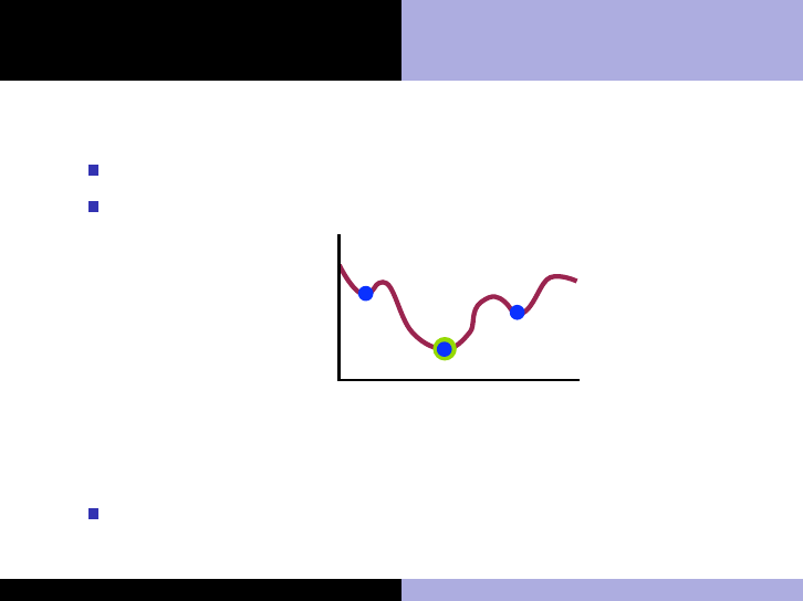
Convex v. non-convex significance
Convex: a unique optimum (local solution=global solution)
NLP: A global optimum is desired, but can be difficult to find
f(x)
x
Figure: Local and global solutions for a nonlinear objective function.
Local optimization algorithms can be used to find the global
optimum (from different starting points) for NLPs
Kevin Carlberg Lecture 1: Introduction to Engineering Optimization

Outline
Motivation
Example
Problem Classification
Modeling
Convex v. non-convex
Continuous v. discrete
Constrained v. unconstrained
Single-objective v. multi-objective
Continuous v. discrete optimization
Discrete: The feasible set is finite
Always non-convex
Many problems are NP-hard
Sub-types: combinatorial optimization, integer programming
Example: How many warehouses should we build?
Continuous: The feasible set is uncountably infinite
Continuous problems are often much easier to solve because
derivative information can be exploited
Example: How thick should airplane wing skin be?
Discrete problems are often reformulated as a sequence of
continuous problems (e.g. branch and bound methods)
Kevin Carlberg Lecture 1: Introduction to Engineering Optimization

Outline
Motivation
Example
Problem Classification
Modeling
Convex v. non-convex
Continuous v. discrete
Constrained v. unconstrained
Single-objective v. multi-objective
Constrained v. unconstrained
Unconstrained problems (n
e
= n
i
= 0) are usually easier to
solve
Constrained problems are thus often reformulated as a
sequence of unconstrained problems (e.g. penalty methods)
Kevin Carlberg Lecture 1: Introduction to Engineering Optimization

Outline
Motivation
Example
Problem Classification
Modeling
Convex v. non-convex
Continuous v. discrete
Constrained v. unconstrained
Single-objective v. multi-objective
Single-objective v. Multi-objective optimization
We may want to optimize two competing objectives f
1
and f
2
(e.g. manufacturing cost and performance)
Pareto frontier: set of candidate solutions among which no
solution is better than any other solution in both objectives
f
1
f
2
These problems are often solved using evolutionary algorithms
Kevin Carlberg Lecture 1: Introduction to Engineering Optimization

Outline
Motivation
Example
Problem Classification
Modeling
Modeling
Modeling: the process of identifying the objective, variables,
and constraints for a given problem
Modeling
Algorithm
selection
Parameter
selection
Solution
Yes
No
Makes sense?
Finished
The more abstract the problem, the more difficult modeling
becomes
Kevin Carlberg Lecture 1: Introduction to Engineering Optimization

Outline
Motivation
Example
Problem Classification
Modeling
Example (Homework)
You live in a house with two other housemates and two
vacancies. You are trying to choose two of your twenty mutual
friends (who all want to live there) to fill the vacancies.
? ?
Model the problem as a mathematical optimization problem,
and categorize the problem as constrained/unconstrained,
continuous/discrete, convex/NLP, and single/multi-objective
Kevin Carlberg Lecture 1: Introduction to Engineering Optimization

