Traffic Safety Program Evaluation: The Empirical Bayes Model and

Traﬃc Safety Program Evaluation: The Empirical Bayes Model

and Mean Reversion Bias

Paul J. Fisher

Independent Researcher

Justin Gallagher

Montana State University

November 23, 2023

Abstract

Motor vehicle fatalities are increasing in the US. The US Department of Transportation

emphasizes the need to implement “proven safety countermeasures,” to reverse the

“crisis on America’s roadways.” Separating the causal safety eﬀect of a traﬃc policy

from the natural variation in crash rates is challenging. The empirical bayes (EB) model

was developed to correct for regression to the mean estimation bias and is a standard,

widely used methodology in the traﬃc safety engineering literature. We show that the

EB model does not correct for regression to the mean bias. We show this analytically,

via a placebo Monte Carlo experiment, and in reference to the traﬃc safety literature.

We demonstrate the shortcomings of the EB model and our recommendations for how

to improve the reliability of traﬃc safety studies using 20 years of data (2003-2022) on

all vehicle crashes in San Antonio, TX.

Keywords: Traﬃc Safety, Mean Reversion, Empirical Bayes, Red-light Cameras

Contact information: [email protected]. We thank Taurey Carr, Max Ellingsen, Elliane Hall, and Sadiq

Salimi Rad for excellent research assistance. The project beneﬁted from conversations with Ahmed Al-Kaisy and feedback from

seminar participants at Montana State University.

“The empirical Bayes (EB) method for the estimation of safety increases the

precision of estimation and corrects for regression-to-mean bias.”

- Hauer et al. (2002), Transportation Research Record, p126

“The EB method pulls the crash count towards the mean, accounting for RTM

bias.”

- US Department of Transportation (2023), Highway Safety Improvement Program

Manual - Safety, p4

1 Introduction

Motor vehicle fatalities are increasing in the US. Fatalities increased by 10.5% from 2020 to

2021. The fatality rate is 18% higher than in 2019 (National Highway Traﬃc Safety Ad-

ministration [2022]). The US Transportation Secretary referred to this reversal in roadway

safety as a “crisis on America’s roadways” (National Highway Traﬃc Safety Administra-

tion [2022b]). The US Department of Transportation (USDOT) emphasizes the need to

implement “proven safety countermeasures” to meet this crisis (USDOT [2023]).

Regression to the mean (RTM) is a well-known challenge in measuring roadway risk and in

evaluating the eﬀectiveness of safety countermeasures (USDOT [2023b]). Naturally occurring

variation in the number of crashes can be misinterpreted as evidence that a traﬃc intervention

improves safety (e.g., Gallagher and Fisher [2020]). Roadway safety interventions often occur

following years when there is an unusually high number of crashes. We would expect the

number of crashes to be lower the following year, regardless of whether there is any safety

intervention.

Separating the causal safety eﬀect of a traﬃc policy from the natural variation in crashes

is challenging. The empirical bayes (EB) model was developed to correct for RTM estimation

bias (e.g., Abbess et al. [1981]; Hauer [1986]). The EB model is a standard, widely used

methodology in the traﬃc safety engineering literature. The popularity of the EB model

stems from the belief that the model “corrects” for RTM bias (e.g., Hauer et al. [2002],

p126). The EB model is the preferred research methodology for both the USDOT and

the American Association of State Highway and Transportation Oﬃcials (Highway Safety

Manual [2023], Section 3). The USDOT recommends the EB model to “control for RTM”

(USDOT [2007], p3) and asserts that the EB method “account[s] for RTM bias” (USDOT

[2023c], p4).

We show that the EB model does not correct for RTM bias. The EB model can lessen

RTM bias, but never fully account for the bias. Moreover, the EB model, as commonly

applied in the transportation and safety engineering literature, corrects for very little RTM

bias. We ﬁrst show this analytically. Next, we run a placebo Monte Carlo policy experiment.

Our Monte Carlo analysis shows that the EB model performs particularly poorly when there

is a high amount of unexplained variation in the crash data and when researchers select

modeling weights to produce the most eﬃcient estimator.

In Section 5, we evaluate a placebo traﬃc intersection safety program using twenty years

of data (2003-2022) on all vehicle crashes in San Antonio, TX, the 12th largest city in North

America. We refer to this non-existent safety intervention as a “placebo red-light camera

program,” although the placebo policy could be any intersection safety countermeasure.

Red-light camera (RLC) programs are common in US cities. San Antonio is one of the

few large cities never to have had a RLC program (Insurance Institute for Highway Safety

[2023]). Meta-analyses, which almost exclusively summarize studies that use the EB model,

conclude that RLC programs dramatically reduce the number of total crashes (Høye [2013];

Goldenbeld et al. [2019]). We show that a simple before-after model implies a 12% reduction

in total crashes, when intersections are selected for the placebo treatment using selection

criteria similar to that used in other cities with actual RLC programs. We then show that

the standard EB model does not correct for mean reversion in this setting. The EB model

is severely biased towards ﬁnding that RLC programs improve safety.

The USDOT rightly states that “program and project evaluations help agencies deter-

mine which countermeasures are most eﬀective in saving lives and reducing injuries” (USDOT

[2023c], p16). However, policy evaluations are only helpful if they provide unbiased estimates

for the causal impact of the safety measure being studied. The ﬁnal section provides recom-

mendations for how to improve the reliability of traﬃc safety studies, given that researchers

can not rely on the EB model to correct for RTM bias. We propose diagnostic tests that

will help researchers gauge the potential RTM bias from using an EB model in a particular

setting. We also draw a parallel to the program evaluation literature in labor economics,

which confronted a similar sample selection problem (e.g., Ashenfelter [1978]; Ashenfelter

and Card [1985]; LaLonde [1986]). The solutions proposed by this literature are illustrative:

the importance of transparent analysis of the raw data, recognition that conventional models

do not solve RTM (and sample selection) bias, an emphasis on careful sample construction,

and the development of new research designs.

2 The Empirical Bayes Model

Road locations targeted for safety countermeasures are not randomly selected. The main

selection concern is that roadway locations (i.e. road segments or intersections) where safety

measures are implemented (“treated” locations) are often chosen based on their underlying

crash risk, or because of recent trends in the number of crashes. Model estimates for how a

safety measure impacts the number of crashes will generally be biased when the underlying

risk diﬀerences are not taken into account, or when naturally occurring variation in the

number of crashes is misinterpreted as part of the causal safety treatment eﬀect.

Treated roadway locations are often selected due to the large number of recent crashes.

A simple before-after model that evaluates the eﬀectiveness of the safety countermeasure

using the time period just before the treatment as the baseline level of crashes will lead to a

safety treatment estimate that is too large. The reason is that the baseline level of crashes

is artiﬁcially high due to naturally occurring variation in the number of crashes. The EB

model (e.g., Abbess et al. [1981]; Hauer [1986]; Hauer et al. [2002]) seeks to account for

this bias by adjusting the baseline level of crashes downwards at treated locations, so as to

eliminate RTM bias and to estimate an unbiased treatment eﬀect.

Below we highlight the key steps to estimate the EB model. In the next section, we

provide details for our two main criticisms of the EB model: (1) the EB model does not

correct for RTM bias, and (2) as applied in the literature, the EB model will usually adjust

for only a small amount of RTM bias.

The ﬁrst step to estimate the EB model is to specify a structural model of vehicle crashes,

referred to as the Safety Performance Function (SPF).

The SPF is supposed to accurately

characterize the deterministic relationship between the number of crashes and the variables

that cause these crashes. The SPF is estimated using out-of-sample data. The traﬃc en-

gineering literature usually estimates the SPF with a negative binomial regression. The

estimated SPF parameters are then applied to the sample locations to generate predictions

for the pre-treatment and post-treatment number of crashes,

E(k

) and

E(λ

), respectively.

Note that in the EB model, there is no diﬀerence between sample locations and treated loca-

tions. The entire sample is comprised of locations where the safety measure is implemented.

Next, use the predicted number of crashes for the sample locations in the pre-treatment

period to adjust the actual crashes observed at these locations. This is the key modeling

step. The adjustment is supposed to account for random variation in the number of crashes

at sample locations that would otherwise lead to RTM bias. In practice, this is done by

calculating a weighted average of the actual and predicted number of crashes (Equation 1).

is the actual number of crashes at the sample locations during the pre-period. ˆw

∈ (0, 1)

is the weight.

E(k

) = ˆw

E(k

) + (1 − ˆw

(1)

Throughout our discussion we assume that all roadway locations are a constant length (e.g. an intersec-

tion or a 1km road segment). See Hauer [1997], Hauer et al. [2002], and Highway Safety Manual [2023] for

detailed discussions on how to estimate the model, including: framing the estimated treatment eﬀect as the

safety index, and adjustments that are necessary when sample locations are of varying lengths.

Equation 2 shows that ˆw

is a ratio of two components that are estimated using the SPF.

V (k

) is the estimated variance in the number of pre-treatment crashes for sample location

V (k

) =

E(k

)

when estimating the model using a negative binomial regression, where ϕ

is the estimated overdispersion parameter.

ˆw

E(k

)

E(k

) +

V (k

)

1 +

E(k

)

(2)

Equation 3 calculates the predicted crashes at each sample location in the post-treatment

period in the absence of a safety intervention. The assumption is that ˆq

E(λ

)

E(k

)

reﬂects how

the number of crashes would have evolved over time if the location was never treated.

ˆπ

= ˆq

E(k

) (3)

The estimated causal eﬀect of a new traﬃc policy or engineering safety measure on the

number of crashes is calculated as

δ = λ − ˆπ. λ is the sum of the actual number of crashes

at sample locations in the post-treatment. ˆπ is the sum of predicted crashes at sample

locations in the post-treatment. The average causal eﬀect of implementing a safety measure

at a sample location is

δ =

λ −

ˆπ, where

δ =

i=1

(and similarly for

ˆπ and

λ).

an unbiased causal estimate for a safety intervention if ˆπ

is an unbiased estimate for the

predicted crashes at each sample location in the absence of an intervention.

Figure 1: EB Model Causal Eﬀect for a Safety Countermeasure

Figure 1 depicts the EB model for sample location i. The y-axis measures the number

of crashes, while the x-axis is time. The vertical line in the middle of the ﬁgure indicates

the introduction of a safety countermeasure (treatment). The points to the left (right) of

the vertical line are calculated over the entire pre-treatment (post-treatment) period. The

estimated causal eﬀect of the safety countermeasure is represented by the vertical distance

between ˆπ

and λ

. We illustrate the case where there is no change in the expected number

of crashes (i.e. ˆq

= 1) and ˆw

is approximately 0.5.

3 The Empirical Bayes Model and RTM Bias

The EB model does not correct for RTM bias. There are two related reasons. First, the

modeling of the SPF. Second, how the EB model ostensibly corrects for mean reversion.

In our discussion, we reference a sample of forty research papers from the published traﬃc

safety engineering literature. We select the papers based on citation counts to highlight the

large variety of safety interventions evaluated using the EB model (Table 1).

3.1 Modeling the Safety Performance Function

The EB model relies on the correct speciﬁcation of the SPF. Estimates from the SPF are

used as a way to reduce RTM bias, and to adjust the observed crash data for calendar time

trends. Numerous driver, vehicle, and roadway factors correlate with crash risk and fatality

rates (e.g., World Health Organization [2022]). However, many EB models estimate a very

parsimonious SPF. The median number of independent crash risk variables included in the

SPF models for the papers in our literature review is two.

In our view, there are two likely reasons why researchers tend to include so few explana-

tory variables when modeling crashes. First, methodological papers often demonstrate the

EB model using a parsimonious SPF. Hauer et al. [2002], a highly cited tutorial, speciﬁes

the SPF using just a single independent variable. Second, in most research settings, detailed

data are unavailable for many factors that correlate with crash rates.

A direct consequence of estimating a SPF with few explanatory variables is that the SPF

is likely to do a poor job explaining the observed variation in crashes. Only 30% of the

studies in our literature review report the amount of crash variation explained by the SPF

model. For example, only around half the crash variation is explained by the SPF models

in Montella et al. [2015]. This is a concern because the SPF is the main modeling tool to

reduce RTM bias.

Roadway locations selected for safety interventions tend to be more risky, on average,

than unselected locations. The EB model applies SPF coeﬃcient estimates that are typically

estimated from lower risk out-of-sample locations to predict crash levels at riskier sample

Table 1: Empirical Bayes Model Literature Review, EB Model Language

Study Topic

EB Model and RTM bias language

Himes et al. (2016) Accident Prevention Tech.

"this methodology is considered rigorous in that it accounts for regression to the mean" p9

Rahman et al. (2020) Accident Prevention Tech.

"the present study used the EB method […] as it accounts for the regression-to-mean bias" p51

Claros et al. (2015) Alternative Intersections

"to account

for […] resulting regression to the mean, the Highway Safety Manual recommends […] empirical Bayes" p6

Edara et al. (2015) Alternative Intersections

"an empirical Bayes analysis to account

for regression to the mean" p12

Gross et al. (2013) Alternative Intersections

"empirical Bayes (EB) methodology to control for regression-to-the-mean" p235

Le et al. (2017) Cost-Benefit Analysis

"EB method is considered rigorous in that it accounts for regression to the mean" p81

Jung (2017) Driving Behavior

"EB and FB methods can increase the precision of the estimation and correct for the regression-to-the-mean bias" p358

Montella (2010) Hot Spot Identification

"EB method increases the precision of the safety estimation and corrects for the regression-to-mean bias" p577

Persaud et al. (2010) Methodology

"this procedure accounts for regression-to-the-mean effects" p38

Yu et al. (2014) Methodology

None

Brewer et al. (2012) Passing Zones

None

Park et al. (2012) Passing Zones

"empirical Bayes (EB) method […] is superior to other methods because it can address

the regression-to-the-mean bias" p38

Persaud et al. (2013) Passing Zones

"because of changes in safety [...] from regression to the mean [...] the count of crashes before a treatment by itself is not a good estimate" p60

Gouda et al. (2020) Pavement Quality

"the before-and-after EB technique […] accounts for critical analysis limitations […] such as regression-to the-mean (RTM)" p93

Park et al. (2017) Pavement Quality

"CMFs [developed using empirical Bayes] can account for the regression-to-the-mean threat" p78

Peel et al. (2017) Pavement Quality

"empirical Bayes […] accurately reflects anticipated changes in crash frequencies […] that may be attributable to regression to the mean bias" p12

Park et al. (2015) Pedestrian, Cyclist Safety

"The main advantage of the EB method is that it can account for […] regression-to-the-mean (RTM) effects" p181

Strauss et al. (2015) Pedestrian, Cyclist Safety

None

Strauss et al. (2017) Pedestrian, Cyclist Safety

None

Goh et al. (2013) Public Transportation

"[empirical Bayes method] key strength is its ability to account

for regression to the mean (RTM) effects" p43

Naznin et al. (2016) Public Transportation

"using the empirical Bayes (EB) method […] account[s] for wider crash trends and regression to the mean effects" p91

Ahmed et al. (2015) Red Light Cameras

"to account for the possible regression-to-the-mean (RTM) bias […] Empirical Bayes (EB) method should be adopted" p133

Ko et al. (2017) Red Light Cameras

"this study uses an EB methodology to address

regression-to-mean (RTM) bias" p118

Pulugurtha et al. (2014) Red Light Cameras

"EB method […] minimizes the regression-to-mean bias in a sample and gives valid results even for small samples" p11

Park et al. (2019) Road Signage

"EB methods have been regarded as statistically defensible methods that can cope

with […] regression-to-the-mean bias" p3

Wood et al. (2020) Road Signage

None

Wu et al. (2020) Road Signage

"before-and-after evaluation with the EB method, as proposed by Hauer, which explicitly addresses the RTM effect" p423

Cafiso et al. (2017) Road Shoulders, Barriers

"The methodology [empirical Bayes] has the great advantage to account for the regression to the mean effects" p324

Chimba et al. (2017) Road Shoulders, Barriers

"The EB uses before-and-after procedures which properly account for regression to the mean bias"

Park et al. (2012) Road Shoulders, Barriers

"The EB method can account for the effect of regression-to-the mean" p318

Park et al. (2016) Road Shoulders, Barriers

"main advantage of the EB method is that it can account for […] regression-to-the-mean effects" p33

Khan et al. (2015) Rumble Strips

"[EB method] address[es] the limitation of the Naïve and CG Methods by accounting for the regression-to-the-mean effect" p36

Park et al. (2015) Rumble Strips

"main advantage of the EB method is that it can account for […] regression-to-the mean (RTM) effects" p313

Park et al. (2014) Rumble Strips

"main advantage of the EB method is that it can account for […] regression-to-the mean (RTM) effects" p170

De Pauw et al. (2018) Speed Limits, Enforcement

"EB approach increases the precision of estimation and corrects for the regression-to the-mean (RTM) bias" p85

Montella et al. (2012) Speed Limits, Enforcement

"the empirical Bayes methodology […] properly accounts for regression to the mean" p17

Montella et al. (2015) Speed Limits, Enforcement

"this [empirical Bayes] methodology is rigorous and properly accounts for regression-to-the-mean" p168

Jin et al. (2021) Turn Lanes, Traffic Signals

None

Khattak et al. (2018) Turn Lanes, Traffic Signals

"The E-B method eliminates regression to the mean (RTM) bias" p124

Srinivasan et al. (2012) Turn Lanes, Traffic Signals

"state-of-the-art before-after empirical Bayes method because it has been shown to properly account for regression to the mean" p109

Studies were selected based on topic and citation count from the following journals (2010-2022): Accident Analysis & Prevention, Analytic Models

in Accident Research, Journal of Safety Research, Traﬃc Injury Prevention, Transportation Research Record, Transportation Research Part A-F,

Transportation Science.

locations. The sample and out-of-sample locations are likely to diﬀer based on one or more

of the many crash risk factors omitted from the SPF. This will generally lead the crash risk

parameters estimated on the out-of-sample locations to be biased estimators for the sample

locations (e.g., LaLonde [1986]; Greene [2003]). EB model adjustments for mean reversion

and the passage of time that rely on the SPF will also be biased.

3.2 Adjusting for Mean Reversion

The vast majority of EB studies in our literature review include statements claiming that the

model “corrects” or “accounts” (or similar) for mean reversion (Table 1). These statements

repeat the language used by leading EB model advocates (Hauer et al. [2002]; USDOT

[2023c]).

Equation 1 is the key modeling step that adjusts for mean reversion. Equation 1 calculates

a weighted average of the actual and predicted number of pre-treatment crashes at sample

locations. The assumption is that the SPF will provide an estimate,

E(k

), that is non-mean

reverting and unbiased. Even if this assumption is true, Equation 1 will only eliminate mean

reversion when all of the weight, ˆw

, is on the predicted number of crashes. The weighted

average will be mean reverting when the pre-treatment crash levels are mean reverting and

ˆw

∈ (0, 1).

Figure 2 depicts the two potential sources of bias (SPF misspeciﬁcation and RTM) in the

EB model. The ﬁgure is similar to Figure 1, except that the plotted points are for a sample

of locations, rather than for a single location and the points in the ﬁgure are averages across

the sample.

The vertical distance between

K and

E(k

)

T rue

in Figure 2 shows the anticipated mean

reversion that will occur in years following a safety intervention at treated locations when the

SPF is correctly estimated, regardless of the actual eﬀectiveness of the safety intervention.

The ﬁgure shows three estimates for the average causal eﬀect for a safety countermeasure

using the EB model. The true causal eﬀect is shown by the vertical line (1). The EB model

only provides an unbiased estimate when the SPF is correctly speciﬁed and all of the weight

in Equation 1 is on the SPF estimate for all sample locations. Vertical line (2) shows how the

causal eﬀect will suﬀer from RTM bias, even when the SPF is correctly speciﬁed. Vertical

line (3) shows how the causal eﬀect can be biased from SPF misspeciﬁcation. Note that we

illustrate the case where there is no change in the expected number of crashes (i.e. ˆq

= 1)

and ˆw

is 0.5 for all sample locations. Our critique of the EB model holds for any value of

ˆq

and for ˆw

∈ (0, 1).

Figure 2: EB Model RTM and SPF Misspeciﬁcation Bias

3.3 EB Model Only Reduces a Small Amount of RTM Bias

Equation 2 shows how the weight, ˆw

, is calculated. This equation is used to calculate the

weight because it minimizes the variance of

E(k

) (e.g., Hauer [1997]). In practice, the

EB model is generally estimated with a small ˆw

. The reason is that high crash locations are

most likely to be selected for an intervention. High crash locations have a larger expected

crash to overdispersion parameter ratio (

E(k

)

), as compared to other potential locations.

A small ˆw

implies that the (mean-reverting) number of crashes is weighted more heavily

when calculating the expected number of crashes at sample locations (see Equation 1).

None of the studies from our detailed review specify the average weights used in the SPF.

For example, Ko et al. [2017] evaluate the city of Houston’s red-light camera program. RTM

bias is a serious concern in this setting. Houston oﬃcials selected signal intersections for the

red-light camera safety intervention based on the unusually high number of crashes at these

intersections in the years just prior to the start of the program (e.g., Gallagher and Fisher

[2020]; Stein et al. [2006]). The number of crashes at these Houston intersections would be

expected to decrease in subsequent years due to mean reversion regardless of the camera

program.

We estimate the EB model on our own sample of Houston red-light camera intersections,

using a parsimonious SPF model similar to that of Ko et al. [2017]. We calculate an average

ˆw

less than 0.1. The EB model only eliminates a very small amount of RTM bias.

4 Monte Carlo Simulation Experiment

We generate crash data and simulate a placebo experiment to evaluate the eﬀectiveness of

the EB model at correcting for RTM bias.

4.1 Data Generating Process

We follow the literature and model crashes using a negative binomial distribution. We

generate crash data using Equation 4. The number of crashes at a location is positively

correlated with Average Daily Traﬃc (ADT). ADT

is constant over time at the location

level, drawn from an exponentiated uniform distribution, and can be interpreted as the

number (in hundreds of thousands) of vehicles passing through a location each day.

Crashes

= poisson(gamma



exp(α + 0.05ADT

)



, ϕ) (4)

The overdispersion parameter, ϕ, allows for the variance in the number of crashes to be

larger than the variance for a poisson distribution with the same mean (e.g., Cameron and

Trivedi [2005]). The overdispersion parameter is a key input into the recommended weight

commonly used in the EB model literature (Equation 2). Typically, greater overdispersion

implies a larger crash variance and a smaller ˆw

In our simulations, we vary ϕ to isolate how ˆw

aﬀects RTM bias in the EB model, while

holding the crash variance constant across the generated datasets.

We select α conditional

on ϕ to generate weights, while holding the crash variance constant. We simulate crash data

using 56 diﬀerent values of the overdispersion parameter that lead to ˆw

∈ (0, 0.97], and

create one hundred datasets for each of the 56 parameterizations. Each dataset includes

10,000 locations (i) and six time periods (t) for a total sample size of 60,000.

4.2 Placebo Safety Policy Experiment

We estimate the eﬀect of a placebo safety policy with a true eﬀect of zero using a before-

after model and the EB model. The Monte Carlo experiment focuses on potential RTM bias,

since the estimated SPF matches the true crash data generating process. We assume that a

placebo safety policy is implemented following period three. The ﬁrst three time periods are

considered “pre-policy”, while periods four to six are “post-policy”. The placebo treatment

We also run a Monte Carlo simulation that allows the crash variance to diﬀer between datasets. The

(poor) performance of the EB model in eliminating RTM bias is very similar.

is assigned to the 500 locations with the highest number of crashes in the three pre-policy

periods. These 500 locations comprise our treatment sample in each dataset, while the other

9,500 locations are the out-of-sample locations used to estimate the SPF.

We chose the panel length based on the recommendation in the literature that using the

three most recent pre-policy years are suﬃcient to reliably estimate the EB model. In fact,

conﬁdence in the EB model to eliminate RTM bias, combined with a concern that earlier

years may not reﬂect a location’s current underlying crash risk, lead many researchers to

avoid the use of crash information for earlier years (e.g., Hauer et al. [2002]).

The USDOT motivates the EB model as best practice by stating that the EB model

“account[s] for RTM bias” that would otherwise occur when using a “naive” before-after

model (USDOT [2023c]). In our setting, estimates from a before-after model wrongly suggest

that the placebo policy reduces vehicle crashes. This follows from the fact that there is no

actual safety policy, and because the sample locations are selected based on an unusually

high number of pre-policy crashes. The number of crashes is lower after the placebo policy

due to mean reversion. The average before-after model estimate across our Monte Carlo

samples is approximately -80%.

Figure 3a shows the results of our simulation. We follow the USDOT and use a before-

after model as a baseline to measure whether the EB model corrects for RTM bias (USDOT

[2023c]). The vertical axis plots the ratio of the EB estimate to the before-after model

estimate for the same sample and simulation. We interpret the y-axis as the percentage

of mean reversion remaining when using the EB model. The x-axis measures the average

SPF weight (

ˆw

) used for each sample and simulation. There is a clear negative correlation

between the SPF weight and the level of RTM bias. As expected, EB models that use small

weights correct for very little RTM bias.

5 San Antonio Crash Analysis

The San Antonio analysis is motivated by the EB modeling literature, which concludes that

red-light camera programs are highly eﬀective in reducing the total number of crashes (e.g.,

Høye [2013]; Goldenbeld et al. [2019]). We demonstrate the shortcomings of the EB model

in correcting for RTM bias using 20 years (2003-2022) of data on all reported vehicle crashes

in San Antonio, TX.

5.1 Data

The crash data are from the Texas Department of Transportation’s Crash Records Infor-

mation System (CRIS) database. CRIS stores information on all TX vehicle crashes. The

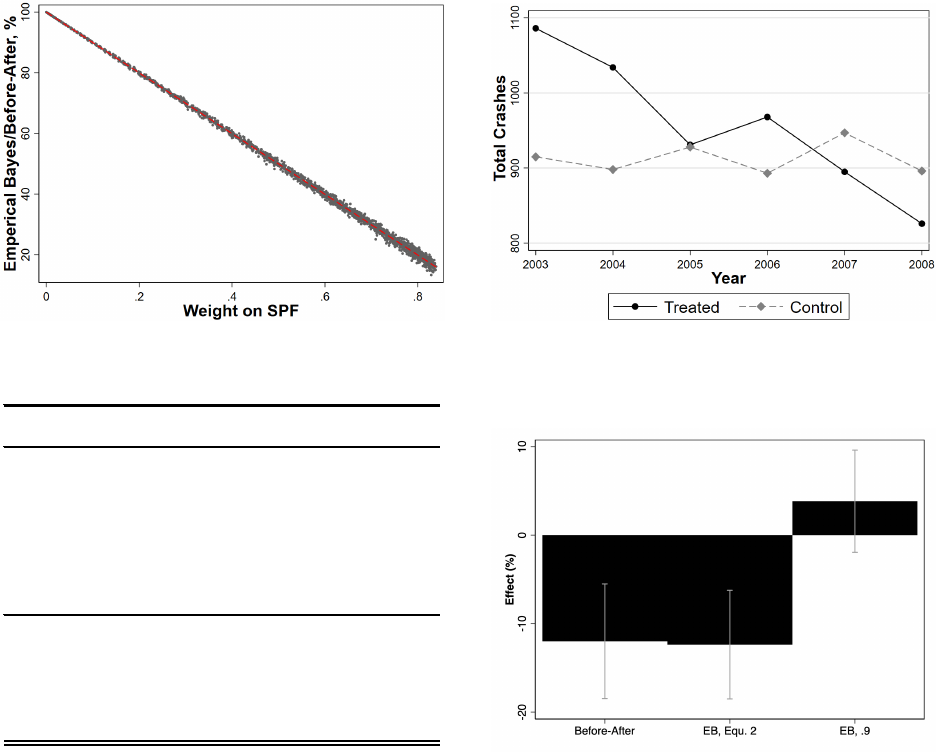
Figure 3: Monte Carlo and San Antonio Placebo Policy Analyses

(a) Remaining RTM Bias (b) Crash Trends in San Antonio, TX

Dependent Variable: Total Crashes

Average Daily Traffic -0.0000026

(0.0000067)

Risk Proxy

0.077

(0.021)

Psuedo R-Squared 0.042

Overdispersion 0.15

Avg weight, treated obs 0.139

Observations 44

information in CRIS is compiled by law enforcement personnel and includes the crash loca-

tion (latitude and longitude) and whether the crash was “in or related to” an intersection.

We use GIS software to identify the yearly count of crashes that are “in or related to” one of

624 major San Antonio intersections. Next, we spatially join all georeferenced crashes that

are within 200 feet of a major intersection and within 50 feet of an intersecting road that

passes through the intersection. We deﬁne an intersection crash as within 200 feet based

on evidence that the number of crashes within 200 feet of an intersection in Houston, TX

during the same time period is several times higher than at any distance greater than 200

feet (Gallagher and Fisher [2020]).

We also collect average daily traﬃc (ADT) information for each intersection (North

Central Texas Council of Governments [2016]). Not all roadways are surveyed each year.

ADT, calculated as the average across all intersecting roads at an intersection, is available

once for each intersection during the ﬁrst three years of our panel. The ﬁnal panel for

our analysis is a yearly intersection-level database that sums the number of crashes at each

intersection.

5.2 Placebo Safety Policy

San Antonio is one of the few large North American cities never to have had a red-light

camera program (Insurance Institute for Highway Safety (2023)). RLC programs use video

cameras to monitor signalized intersections for red-light running. The aim is to reduce

the total number of crashes, and especially injury-related crashes, through a reduction in

collisions involving vehicles running a red light. We focus our analysis on 2003-2008 because

ADT is available for each intersection 2003-2005. We evaluate a placebo intersection safety

countermeasure that we call a RLC program. We assume the policy is implemented in 2006.

We assign the placebo safety intervention to the 50 intersections with the largest number of

crashes 2003-2005. This selection criteria closely follows how Houston selected intersections

for its RLC program (Stein et al. [2006]; Gallagher and Fisher [2020]). The eﬀect of the

program is analyzed using three post-treatment years 2006-2008.

Figure 3b plots the total number of crashes at the “treated” and “control” intersections

by year. The number of crashes is stable at the control intersections before and after the

placebo safety policy. The average total number of yearly crashes at the control intersection

is 914 before the policy and 912 after the policy. In sharp contrast, the number of crashes

at treated intersections decreased by 12% from 1,017 pre-policy to 896 post-policy.

5.3 Model Results

We evaluate the placebo program using a simple before-after model and the EB model. The

before-after model implies that the program led to a 12% reduction in crashes (Figure 3d).

The entire estimated reduction in the before-after model is due to mean reversion. There is

no evidence of an overall trend in crashes at the non-treated intersections (Figure 3b).

Our review of two recent meta-analyses on the safety eﬀectiveness of RLC programs

reveals that most of these studies use the EB model and a parsimonious SPF ([Høye, 2013];

[Goldenbeld et al., 2019]). The median number of independent variables in the SPF is two.

ADT is included in every SPF. We follow the literature in our analysis and also specify an

SPF with two independent variables and include ADT as one of the variables. The second

variable in our SPF is a proxy for crash risk, measured as the yearly mean number crashes at

the intersection from 2003-2022. Twenty years of actual crash data provides a good measure

of the true crash risk at each intersection. The variable is a proxy because it does not reﬂect

changes to the roadways or city-wide driving patterns that may have altered the underlying

crash risk. We do not claim to have modeled a correct SPF. Our aim is to specify a SPF

model in line with the current literature.

A critical decision in any EB model analysis is how to specify the control group when

estimating the SPF. The crash-related characteristics of the control group should closely

match those of the treated group. We use the risk proxy variable to limit out-of-sample San

Antonio control intersections to those with a risk proxy in the same range as the treated

intersections. All potential control intersections with an average number of yearly crashes

(2003-2022) of less than 5.0 or greater than 29.4 are excluded from the analysis. We estimate

the SPF on a sample of 44 control intersections.

Figure 3c shows results from using a binomial regression to estimate our SPF. The table

lists parameter estimates and standard errors (in parentheses) for the independent variables.

The estimated coeﬃcients can be interpreted as semi-elasticities. We estimate that a one

crash per year increase in the risk proxy increases the average number of yearly crashes at the

intersection in the placebo pre-period (2003-2005) by approximately 8 percent (probability

value < 0.01).

Figure 3d displays the before-after and EB model point estimates. We estimate the

EB model using two diﬀerent sets of model weights ( ˆw

). The recommended approach in

the literature is to use Equation 2 to determine ˆw

for each treated intersection. When we

use the recommended approach, we estimate an average weight of 0.14 (Figure 3c), and a

placebo policy treatment eﬀect of -12% (Figure 3d, middle column). The ﬁgure shows the

95% conﬁdence interval in brackets.

The EB model estimate is very similar to the before-

after estimate. Both estimates suﬀer from substantial RTM bias. In the third column of

Figure 3d we estimate the EB model using a ﬁxed weight of 0.9 for all intersections. The

estimated average placebo safety treatment eﬀect is small in magnitude and not statistically

diﬀerent from zero.

6 Discussion and Recommendations

We provide the following recommendations for researchers and practitioners who continue

to use the EB model, or who seek alternative models to evaluate traﬃc safety interventions.

6.1 Better Selection of Intervention Sites

Safety interventions should target high risk road locations to most improve roadway safety.

However, a treatment selection process where the selection criteria emphasize recent spikes

We calculate bootstrapped standard errors using a non-parametric bootstrap procedure and 1,000 boot-

strap samples (e.g., Efron and Tibshirani [1993]; Cameron and Trivedi [2005]).

in crashes, rather than the underlying crash risk, will lead to mean reversion and complicate

evaluation of the safety intervention.

Mean reversion induced by the site selection method can be reduced by limiting the role

that year-to-year variation in crash outcomes plays in selecting treatment locations. First,

select locations for a safety intervention using more years of crash data (e.g. 10 years rather

than 2-3 years as is common). Second, practitioners can minimize selection based on mean

reverting temporal trends by excluding the most recent crash data (e.g., Ashenfelter [1978]).

This is in direct contrast to the current recommendation in the EB modeling literature

(e.g., Hauer et al. [2002]). Third, avoid using infrequent crash outcomes, such as fatalities,

to measure roadway risk when assigning safety interventions. Even the most dangerous

locations often have years with no fatal crashes. An assignment criteria that includes all

crashes, while weighting the more severe crashes, will provide a more stable measure of risk

over time and reduce mean reversion. The most eﬀective method for site selection is to

randomize the intervention across a sample of (pre-selected) locations, and then to evaluate

the treatment eﬀect using a randomized controlled trial (e.g., Elvik [2021]).

Practitioners can evaluate whether the selection process is likely to lead to treated lo-

cations characterized by mean reversion. Use the site selection criteria to create proposed

lists of treated locations using diﬀerent pre-treatment time periods. If the proposed treat-

ment locations vary substantially from period to period, then the selection criteria is mainly

picking up on temporal trends and doing a poor job measuring the true underlying crash

risk. Locations assigned safety interventions using these criteria will likely be characterized

by mean reversion and assessing the true impact of the safety intervention will be diﬃcult.

6.2 Improved Application of the Empirical Bayes Method

We recommend updating language to better reﬂect the ability of the EB method to reduce

RTM bias, reporting additional statistics regarding mean reversion, and selecting a high

weight ( ˆw

Researchers frequently describe the EB model as “correcting”, “accounting”, “address-

ing”, or “eliminating” RTM bias (Table 1). The Bayesian intuition of combining existing

and new sample information to improve model estimates does not correct for RTM bias. The

EB model will only eliminate RTM bias when the SPF model is speciﬁed correctly and when

all weight is placed on the out-of-sample prediction (i.e. ˆw

= 1). We recommend that re-

searchers are transparent about these limitations of the model. Moreover, researchers should

report the average ˆw

, which provides an indication of the remaining RTM bias relative to

the simple before-after model.

Researchers should set a large weight in the SPF model when there is concern over

mean reversion. The standard approach is to estimate Equation 2, which selects ˆw

minimize the estimated variance of

E(k

) and thereby maximizes the precision of the

EB model. However, there is a trade-oﬀ between the duel objectives of eliminating RTM

bias and maximizing precision. We recommend using a ﬁxed weight of 0.9 in settings where

there is suspected mean reversion. A weight of 1.0 would eliminate RTM bias, provided the

SPF is correctly speciﬁed, but completely relies on out-of-sample prediction. Moreover, a

weight of 1.0 would no longer reﬂect the Bayesian approach of combining existing crash risk

information with new crash risk information from the sample locations targeted for a safety

intervention. A weight of 0.9 allows the EB model to largely reduce RTM bias in expectation

(Figure 3a) and in practice (Figure 3d), while still incorporating location speciﬁc information

not captured by the SPF.

6.3 Consider Alternative Models for Analysis

The diﬀerence-in-diﬀerences (DD) model is an attractive alternative to the EB model (e.g.,

Angrist and Pischke [2008]; Roth et al. [2023]). The DD model estimates the eﬀect of a

safety intervention by comparing the change before and after intervention for treated sites to

the same before and after change for the control sites. The DD model allows the researcher

to adjust for mean reversion by selecting control locations that have similar patterns of mean

reversion as treated locations.

The most important part of the DD model is to choose control locations that would have a

similar change in the number of crashes without the intervention. There are several strategies

to choose control locations. First, if researchers know the criteria used by policy makers to

select the treated locations, then similar control locations can be selected using the same

criteria. For example, there may be control locations that meet the same selection criteria,

but were excluded for reasons unrelated to crash risk (e.g. political or budget considerations).

Second, use propensity score matching and trimming to identify sites with similar features

as those receiving the intervention (e.g., Abdulsalam et al. [2017], Gallagher and Fisher

[2020]). Third, use eligible non-selected locations when the organization implementing the

intervention randomizes the treated locations.

7 Conclusion

The empirical bayes model was developed to correct for regression to the mean estimation

bias and is a standard, widely used methodology in the traﬃc safety engineering literature.

We show that the EB model does not correct for RTM bias. We ﬁrst show this analyti-

cally using the EB modeling equations. The EB model will lead to causal safety measure

estimates that suﬀer from RTM bias, unless the EB model completely ignores crash data

at the treatment locations. Our Monte Carlo analysis shows that the EB model performs

particularly poorly when there is a high amount of unexplained variation in the crash data

and when researchers select modeling weights to produce the most eﬃcient estimator.

We apply the EB model to analyze a placebo traﬃc safety program using twenty years

of data (2003-2022) on all vehicle crashes in San Antonio, TX. We refer to this non-existent

safety program as a red-light camera program. We show that a simple before-after model

implies a 12% reduction in total crashes, when intersections are selected for the placebo

treatment using selection criteria similar to that used in other cities with actual RLC pro-

grams. We then show that the standard EB model does not correct for mean reversion in

this setting.

Our recommendations for how to improve the reliability of traﬃc safety studies include

recognizing that the EB model does not correct for RTM bias, proposed diagnostic tests to

gauge the amount of potential RTM bias from using an EB model, a stronger emphasis on

careful sample construction, and the application of statistical models that are more likely to

correct for RTM bias.

8 References

Automated enforcement: A compendium of worldwide evaluations of results. Technical Report

DOT HS 810 763, Department of Transportation, 2007.

Early estimates of motor vehicle traﬃc fatalities and fatality rate by sub-categories in 2021. Tech-

nical Report DOT HS 813 298, National Highway Traﬃc Safety Administration, May 2022.

Roadway traﬁc injuries. Technical report, The World Health Organization, June 2022. URL

https://www.who.int/news-room/fact-sheets/detail/road-traffic-injuries.

Highway safety manual. Technical report, American Association of State Highway and

Transportation Oﬃcials, 2023. URL https://www.highwaysafetymanual.org/Pages/

ResearchResources.aspx.

National roadway safety strategy. Technical report, Department of Transportation, 2023a. URL

https://www.transportation.gov/NRSS/SaferRoads.

Applying safety data and analysis to performance-based transportatino planning. Technical

report, Department of Transportation, 2023b. URL https://highways.dot.gov/safety/

zero-deaths/transportation-safety-planning-tsp.

Highway safety improvement program manual. Technical report, Department of Transportation,

2023c. URL https://safety.fhwa.dot.gov/hsip/resources/fhwasa09029/sec6.cfm.

Red light running. Technical report, 2023. URL https://www.iihs.org/topics/

red-light-running#communities-using-red-light-safety-cameras.

Christopher Abbess, Daniel Jarrett, and Catherine C. Wright. Accidents at blackspots: Estimating

the eﬀectiveness of remedial treatment, with special reference to the “regression-to-mean” eﬀect.

Traﬃc Engineering and Control, 22(10), 1981.

Amal Jasem Abdulsalam, Dane Rowlands, Said M Easa, and Abd El Halim O Abd El Halim. Novel

case-control observational method for assessing eﬀectiveness of red-light cameras. Canadian

Journal of Civil Engineering, 44, 2017.

National Highway Traﬃc Safety Administration. Newly released estimates show traﬃc fatalities

reached a 16-year high in 2021. US Department of Transportation, May 2022.

Jon Tommeras Selvik adn Rune Elvik and Eirik Bjorheim Abrahamsen. Can the use of road safety

measures on national roads in norway be interpreted as an informal application of the alarp

principle. Accident Analysis & Prevention, 135, 2020.

Mohamed M. Ahmed and Mohamed Abdel-Aty. Evaluation and spatial analysis of automated red-

light running enforcement cameras. Transportation Research Part C: Emerging Technologies, 50,

2015.

Joshua D. Angrist and Jorn-Steﬀen Pischke. Mostly Harmless Econometrics. Princeton University

Press, 2008.

Orley Ashenfelter. Estimating the eﬀect of training programs on earnings. The Review of Economics

and Statistics, 60, 1978.

Orley Ashenfelter and David Card. Using the longitudinal structure of earnings to estimate the

eﬀect of training programs. The Review of Economics and Statistics, 67, 1985.

Marcus A. Brewer, Steven P. Venglar, Kay Fitzpatrick, Liang Ding, and Byung-Junk Park. Super

2 highways in texas: Operational and safety characteristics. Transportation Research Record:

Journal of the Transportation Research Board, 2301, 2012.

Salvatore Caﬁso and Alessandro Di Graziano. Surrogate safety measures for optimizing investments

in local rural road networks. Transportation Research Record: Journal of the Transportation

Research Board, 2237, 2011.

Salvatore Caﬁso, Carmelo D’Agostino, and Bhagwant Persaud. Investigating the inﬂuence on

safety of retroﬁtting italian motorways with barriers meeting a new eu standard. Traﬃc Injury

Prevention, 18, 2017.

A. Colin Cameron and Pravin K. Trivedi. Microeconometrics. Cambridge University Press, 2005.

Deo Chimba, Evarist Ruhazwe, Steve Allen, and Jim Waters. Digesting the safety eﬀectiveness

of cable barrier systems by numbers. Transportation Research Part A: Policy and Practice, 95,

2017.

Mehmet Ali Dereli and Saﬀet Erdogan. A new model for determining the traﬃc accident black

spots using gis-aided spatial statistical methods. Transportation Research Part A: Policy and

Practice, 103, 2017.

Praveen Edara, Sawyer Breslow, Carlos Sun, and Boris R. Claros. Empirical evaluation of j-turn

intersection performance: Analysis of conﬂict measures and crashes. Transportation Research

Record: Journal of the Transportation Research Board, 2486, 2015.

Bradley Efron and R.J. Tibshirani. An Introduction to the Bootstrap. Chapman and Hall, 1993.

Rune Elvik. Why are there so few experimental road safety evaluation studies: Could their ﬁndings

explain it? Accident Analysis & Prevention, 163, 2021.

Justin Gallagher and Paul J. Fisher. Criminal deterrence when there are oﬀsetting risks: Traﬃc

cameras, vehicular accidents, and public safety. American Economic Journal: Economic Policy,

12(3), 2020.

Kelvin Chun Keong Goh, Graham Currie, Majid Sarvi, and David Logan. Road safety beneﬁts from

bus priority: An empirical study. Transportation Research Record: Journal of the Transportation

Research Board, 2352, 2013.

Charles Goldenbeld, Stijn Daniels, and Govert Schermers. Red light cameras revisited. recent

evidence on red light camera safety eﬀects. Accident Analysis & Prevention, 128, 2019.

Maged Gouda and Karim El-Basyouny. Before-and-after empirical bayes evaluation of achieving

bare pavement using anti-icing on urban roads. Transportation Research Record: Journal of the

Transportation Research Board, 2674, 2020.

William H. Greene. Econometric Analysis. Prentice Hall, 2003.

Frank Gross, Craig Lyon, Bhagwant Persaud, and Raghavan Srinivasan. Safety eﬀectiveness of

converting signalized intersections to roundabouts. Accident Analysis & Prevention, 50, 2013.

Ezra Hauer. On the estimation of the expected number of accidents. Accident Analysis & Preven-

tion, 18, 1986.

Ezra Hauer. Observational Before-After Studies in Road Safety. Emerald Group Publishing Limited,

1997.

Ezra Hauer, Douglas W. Harwood, Forrest M. Council, and Michael S. Griﬃth. Estimating safety

by the empirical bayes method: A tutorial. Transportation Research Record, 1784, 2002.

Scott Himes, Frank Gross, Kimberly Eccles, and Bhagwant Persaud. Multistate safety evaluation

of intersection conﬂict warning systems. Transportation Research Record, 2583(1), 2016.

Alena Høye. Still red light for red light cameras? an update. Accident Analysis and Prevention,

55, 2013.

Weimin Jin, Mashrur Chowdhury, Sakib Mahmud Khan, and Patrick Gerard. Investigating the

impacts of crash prediction models on quantifying safety eﬀectiveness of adaptive signal control

systems. Journal of Safety Research, 76, 2021.

Soyoung Jung, Shinhye Joo, and Cheol Oh. Evaluating the eﬀects of supplemental rest areas on

freeway crashes caused by drowsy driving. Accident Analysis & Prevention, 99, 2017.

Mubassira Khan, Ahmed Abdel-Rahim, and Christopher J. Williams. Potential crash reduction

beneﬁts of shoulder rumble strips in two-lane rural highways. Accident Analysis & Prevention,

75, 2015.

Zulqarnain H. Khattak, Mark J. Magalotti, and Michael D. Fontaine. Estimating safety eﬀects of

adaptive signal control technology using the empirical bayes method. Journal of Safety Research,

64, 2018.

Myunghoon Ko, Srinivis Reddy Geedipally, Troy Duane Walden, and Robert Carl Wunderlich.

Eﬀects of red light running camera systems installation and then deactivation on intersection

safety. Journal of Safety Research, 62, 2017.

Robert J. LaLonde. Evaluating the econometric evaluations of training programs using experimental

data. The American Economic Review, 76, 1986.

Thanh Q. Le, Frank Gross, and Timothy Harmon. Safety eﬀects of low-cost systemic safety improve-

ments at signalized and stop-controlled intersections. Transportation Research Record: Journal

of the Transportation Research Board, 2636, 2017.

Alfonso Montella. A comparative analysis of hotspot identiﬁcation methods. Accident Analysis &

Prevention, 42, 2010.

Alfonso Montella, Bhagwant Persaud, Mauro D’Apuzzo, and Lella Liana Imbriani. Safety evaluation

of automated section speed enforcement system. Transportation Research Record: Journal of the

Transportation Research Board, 2281, 2012.

Alfonso Montella, Lella Liana Imbriani, Vittorio Marzano, and Filomena Mauriello. Eﬀects on speed

and safety of point-to-point speed enforcement systems: Evaluation on the urban motorway a56

tangenziale di napoli. Accident Analysis & Prevention, 75, 2015.

Farhana Naznin, Graham Currie, Majid Sarvi, and David Logan. An empirical bayes safety evalua-

tion of tram/streetcar signal and lane priority measures in melbourne. Traﬃc Injury Prevention,

17, 2016.

North Central Texas Council of Governments. Historical traﬃc counts, 2016. URL http://www.

nctcog.org/trans/data/trafficcounts/indexcdp.asp.

Eun Sug Park, Paul J. Carlson, Richard J. Porter, and Carl K. Anderson. Safety eﬀects of wider

edge lines on rural, two-lane highways. Accident Analysis & Prevention, 48, 2012.

Eun Sug Park, Paul J. Carlson, and Adam Pike. Safety eﬀects of wet-weather pavement markings.

Accident Analysis & Prevention, 133, 2019.

Juneyoung Park and Mohamed Abdel-Aty. Development of adjustment functions to assess combined

safety eﬀects of multiple treatments on rural two-lane roadways. Accident Analysis & Prevention,

75, 2015.

Juneyoung Park, Mohamed Abdel-Aty, and Chris Lee. Exploration and comparison of crash mod-

iﬁcation factors for multiple treatments on rural multilane roadways. Accident Analysis & Pre-

vention, 70, 2014.

Juneyoung Park, Mohamed Abdel-Aty, and Jaeyoung Lee. Use of emperical and full bayes before-

after approaches to estimate the safety eﬀects of roadside barriers with diﬀerent crash conditions.

Journal of Safety Research, 58, 2016.

Juneyoung Park, Mohamed Abdel-Aty, and Jung-Han Wang. Time series trends of the safety eﬀects

of pavement resurfacing. Accident Analysis & Prevention, 101, 2017.

Ellan De Pauw, Stijn Daniels, Laurent Franckx, and Inge Mayeres. Safety eﬀects of dynamic speed

limits on motorways. Accident Analysis & Prevention, 114, 2018.

Thomas Peel, Mohamed Ahmed, and Noriaki Ohara. Investigating safety eﬀectiveness of wyoming

snow fence installations along a rural mountainous freeway. Transportation Research Record:

Journal of the Transportation Research Board, 2613, 2017.

Bhagwant Persaud, Bo Lan, Craig Lyon, and Ravi Bhim. Comparison of empirical bayes and full

bayes approaches for before-after road safety evaluations. Accident Analysis & Prevention, 42,

2010.

Bhagwant Persaud, Craig Lyon, Jeﬀrey Bagdade, and Andrew H. Ceifetz. Evaluation of safety per-

formance of passing relief lanes. Transportation Research Record: Journal of the Transportation

Research Board, 2348, 2013.

Srinivas S. Pulugurtha and Ramesh Otturu. Eﬀectiveness of red light running camera enforcement

program in reducing crashes: Evaluation using “before the installation”, “after the installation”,

and “after the termination” data. Accident Analysis & Prevention, 64, 2014.

Moynur Rahman and Min-Wook Kang. Safety evaluation of drowsy driving advisory system: Al-

abama case study. Journal of Safety Research, 74, 2020.

Jonathan Roth, Pedro H.C. Sant’Anna, Alyssa Bilinski, and John Poe. What’s trending in

diﬀerence-in-diﬀerences? a synthesis of the recent econometrics literature. Journal of Econo-

metrics, August 2023.

Raghavan Srinivasan, Craig Lyon, Bhagwant Persaud, Jongdae Baek, Frank Gross, Sarah Smith,

and Carl Sundstrom. Crash modiﬁcation factors for changes to left-turn phasing. Transportation

Research Record: Journal of the Transportation Research Board, 2279, 2012.

Robert Stein, Ned Levine, and Tim Lomax. Criteria for red light camera intersection selection,

2006.

Jillian Strauss, Luis F. Miranda-Moreno, and Patrick Morency. Mapping cyclist activity and injury

risk in a network combining smartphone gps data and bicycle counts. Accident Analysis &

Prevention, 83, 2015.

Jillian Strauss, Sohail Zangenehpour, Luis F. Miranda-Moreno, and Nicolas Saunier. Cyclist de-

celeration rate as surrogate safety measure in montreal using smartphone gps data. Accident

Analysis & Prevention, 99, 2017.

Xuesong Wang, Yilun Xing, Lian Luo, and Rongjie Yu. Evaluating the eﬀectiveness of behavior-

based safety education methods for commercial vehicle drivers. Accident Analysis & Prevention,

117, 2018.

Jonathon Wood and Eric T. Donnell. Empirical bayes before-after evaluation of horizontal curve

warning pavement markings on two-lane rural highways in pennsylvania. Accident Analysis &

Prevention, 146, 2020.

Mingjian Wu, Karim El-Basyouny, and Tae J. Kwon. Before-and-after empirical bayes evaluation

of citywide installation of driver feedback signs. Transportation Research Record: Journal of the

Transportation Research Board, 2674, 2020.

Hao Yu, Pan Liu, Jun Chen, and Hao Wang. Comparative analysis of the spatial analysis methods

for hotspot identiﬁcation. Accident Analysis & Prevention, 66, 2014.

Yingheng Zhang, Haojie Li, N.N. Sze, and Gang Ren. Propensity score methods for road safety

evaluation: Practical suggestions from a simulation study. Accident Analysis & Prevention, 158,

2021.