Site Selection Bias in Program Evaluation

NBER WORKING PAPER SERIES

SITE SELECTION BIAS IN PROGRAM EVALUATION

Hunt Allcott

Working Paper 18373

http://www.nber.org/papers/w18373

NATIONAL BUREAU OF ECONOMIC RESEARCH

1050 Massachusetts Avenue

Cambridge, MA 02138

September 2012

This paper is a substantial revision of a manuscript titled "External Validity and Partner Selection

Bias" on which Sendhil Mullainathan was a co-author. Although he is no longer a co-author, this

project has benefited enormously from his insights. I thank Josh Angrist, Amitabh Chandra, Lucas

Davis, Kyle Dropp, Meredith Fowlie, Xavier Gine, Chuck Goldman, Matt Harding, Joe Hotz, Guido

Imbens, Larry Katz, Chris Knittel, Dan Levy, Jens Ludwig, Konrad Menzel, Emily Oster, Rohini

Pande, Todd Rogers, Piyush Tantia, Ed Vytlacil, Heidi Williams, and seminar participants at the ASSA

meetings, Berkeley, Columbia, Harvard, MIT, NBER Labor Studies, NBER Energy and Environmental

Economics, NEUDC, the UCSB/UCLA Conference on Field Experiments, and the World Bank for

insights and helpful advice. Thanks also to Tyler Curtis, Marc Laitin, Alex Laskey, Alessandro Orfei,

Nate Srinivas, Dan Yates, and others at Opower for fruitful discussions. Christina Larkin provided

timely research assistance. The views expressed herein are those of the authors and do not necessarily

reflect the views of the National Bureau of Economic Research.

NBER working papers are circulated for discussion and comment purposes. They have not been peer-

reviewed or been subject to the review by the NBER Board of Directors that accompanies official

NBER publications.

be quoted without explicit permission provided that full credit, including © notice, is given to the source.

Site Selection Bias in Program Evaluation

Hunt Allcott

NBER Working Paper No. 18373

September 2012, Revised March 2014

JEL No. C93,D12,L94,O12,Q41

ABSTRACT

“Site selection bias” occurs when the probability that partners adopt or evaluate a program is correlated

with treatment effects. I test for site selection bias in the context of the Opower energy conservation

programs, using 111 randomized control trials (RCTs) involving 8.6 million households across the

United States. Predictions based on rich microdata from the first ten replications substantially overstate

efficacy in the next 101 sites. There is evidence of two positive selection mechanisms. First, local

populations with stronger preferences for environmental conservation both encourage utilities to adopt

the program and are more responsive to the treatment. Second, program managers initially target treatment

at the most responsive consumer sub-populations, meaning that efficacy drops when utilities expand

the program. While it may be optimal to initially target an intervention toward the most responsive

populations, these results show how analysts can be systematically biased when extrapolating experimental

results, even after many replications. I augment the Opower results by showing that microfinance institutions

(MFIs) that run RCTs differ from the global population of MFIs and that hospitals that host clinical

trials differ from the national population of hospitals.

Hunt Allcott

Department of Economics

New York University

19 W. 4th Street, 6th Floor

New York, NY 10012

and NBER

[email protected]

1 Introduction

Program evaluation using randomized control trials (RCTs) has long been a important part of

economics, from the Negative Income Tax experiments to the RAND health insurance experiment,

Moving to Opportunity, the Job Training Partnership Act, and a wave of recent RCTs in devel-

opment, health, labor economics, and other ﬁelds. Program evaluation is often used to inform a

policy decision: should a treatment be implemented in some “target” population? Typically, an

evaluation is carried out at one or more sample sites, and the results are generalized to make an

implementation decision in a diﬀerent and often larger set of target sites. This raises questions of

external validity: how well do parameter estimates generalize across sites?

When generalizing empirical results, we either implicitly or explicitly make an assumption I call

external unconfoundedness: that there are no unobservables that moderate the treatment eﬀect and

diﬀer between sample and target. As formalized by Hotz, Imbens, and Mortimer (2005) and Hotz,

Imbens, and Klerman (2006), this type of assumption mirrors the unconfoundedness assumption

required for internal validity (Rosenbaum and Rubin 1983). When we have results from only one

site, this assumption amounts to assuming away the possibility of unexplained site-level treatment

eﬀect heterogeneity. Because this is often unrealistic, we value replication in additional sites. After

enough replications, external unconfoundedness implies only that the distribution of treatment

eﬀects in sample sites can predict the distribution of eﬀects in target sites. Put simply, if an

intervention works well in enough diﬀerent trials, we might advocate that it be scaled up. Formally,

this logic requires that sample sites are as good as randomly selected from the population of target

sites.

In practice, there are many reasons why sites are selected for empirical study. For example,

because RCTs require an implementing partner with managerial ability and operational expertise,

the set of actual partners may be able to run more eﬀective programs than the typical potential

partner. As another example, partners that are already running programs that they know are

eﬀective are more likely to be open to independent impact estimates (Pritchett 2002). Both of these

mechanisms would cause a positive site selection bias: treatment eﬀects from sample sites would

be larger than in the full set of targets. Alternatively, partners that are particularly innovative and

willing to test new programs may also be running many other eﬀective programs in the same area.

If there are diminishing returns, the new program with an actual partner might have lower impact

than with a typical potential partner. This would cause negative site selection bias. Site selection

bias implies that even with a large number of internally valid impact estimates, policymakers could

still draw systematically biased inference about a program’s impact at full scale.

While site selection bias is both intuitive and potentially important, there is little empirical

evidence on this issue or the mechanisms through which it might act. The reason is simple: since

this type of selection operates at the level of the site instead of the individual unit, one needs a

statistically large sample of sites with internally valid estimates of the eﬀect of the same treatment.

Then, one must deﬁne a population of potential partner sites and somehow infer treatment eﬀects

in sites where evaluations have not yet been carried out. Given the cost of RCTs, it is unusual for

the same intervention to be rigorously evaluated at more than a small handful of sites. By contrast,

as in LaLonde (1986), Dehejia and Wahba (1999), Heckman, Ichimura, Smith, and Todd (1998),

Smith and Todd (2004), and many other studies, providing evidence on individual-level selection

bias and an estimator’s internal validity is much less onerous, as it simply requires a large sample

of individuals.

The Opower energy conservation program provides an exceptional opportunity to study the

site selection process. The treatment is to mail “Home Energy Reports” to residential electricity

consumers that provide energy conservation tips and compare their energy use to that of their neigh-

bors. Electric and natural gas utilities have partnered with Opower largely because the program

helps to comply with state-level energy conservation mandates. As of February 2013, the program

had been implemented using 111 randomized control trials involving 8.6 million households at 58

utilities across the United States.

This paper’s organizing question is, what would be the eﬀects if the Opower program were scaled

nationwide? Aside from providing a case study of an important methodological issue, this out-of-

sample prediction problem is also particularly policy-relevant. In recent years, “behavioral” energy

eﬃciency programs have received increasing attention as an alternative to traditional policies such

as subsidies and standards for energy eﬃcient capital stock. While Opower’s home energy reports

are perhaps the most prominent example of such interventions, the American Council for an Energy

Eﬃcient Economy reports that 281 diﬀerent behavior-based programs were run in the U.S. between

2008 and 2013 (Mazur-Stommen and Farley 2013). Consultancy McKinsey & Co. recently released

a study predicting “immense” potential for behavioral energy eﬃciency in the U.S., with potential

savings from Opower and many other opportunities amounting to 16 to 20 percent of current

residential energy consumption (Heck and Tai 2013). Policymakers use such predictions to help

determine the stringency of energy conservation mandates as part of an eﬀort to reduce energy use

externalities and other ineﬃciencies that may increase energy use.

I begin by using microdata from Opower’s ﬁrst ten replications to predict aggregate nation-

wide eﬀects. This is a highly promising opportunity for out-of-sample prediction: there are very

large samples, with 512,000 households in treatment and control, ten diﬀerent replications spread

throughout the country, internally-valid estimates, and a useful set of individual level covariates

to adjust for diﬀerences between sample and target populations. Using the non-parametric test

ENERNOC (2013), KEMA (2013), and Quackenbush (2013) are examples of state-level energy eﬃciency potential

assessments that include predictions for behavioral energy eﬃciency programs based partially on results from RCTs in

pilot locations. The studies were commissioned by utilities and state public utilities commissions as part of the process

of setting Energy Eﬃciency Resource Standards. Allcott and Greenstone (2012) discuss the economic rationale for

these types of policies.

of treatment eﬀect heterogeneity introduced by Crump, Hotz, Imbens, and Mitnik (2008), I show

that treatment eﬀects are larger for households that use more electricity and also vary in intuitive

ways conditional on four other features of a home’s physical capital stock. I then use two standard

“oﬀ-the-shelf” approaches to extrapolation: linear prediction and the re-weighting procedure in-

troduced by Hellerstein and Imbens (1999). Results from these ﬁrst ten replications predict retail

electricity cost savings of about 1.7 percent, or $2.3 billion, in the ﬁrst year of a nationally-scaled

program.

Aside from the microdata, I also have Opower’s “metadata”: impact estimates and standard

errors from all 111 RCTs at all 58 diﬀerent utility partners that began before February 2013. As an

“in-sample” test of external unconfoundedness, I use microdata from the initial ten sites to predict

ﬁrst-year eﬀects at the 101 later sites. The microdata over-predict eﬃcacy by approximately 0.5

percentage points, or $690 million worth of retail electricity. In other words, early sites were strongly

positively selected through mechanisms associated with the treatment eﬀect.

I then focus on the metadata to further document site selection bias and provide suggestive evi-

dence on underlying mechanisms. I use the “site selection probability,” or the conditional probabil-

ity that a utility partners with Opower. There is a close analogy between this site-level propensity

score and the familiar individual-level propensity score, but the “dimension-reduction” property of

propensity scores is particularly useful in meta-analysis with a limited number of site-level observa-

tions. The site selection probability allows a straightforward test of site selection bias: I show that

within the 111 existing RCTs, site selection probabilities are positively associated with treatment

eﬀects. While this association is documented using utility-level observables, I also show that it is

“selection on unobservables” in the sense that it would not have been predicted using the microdata

from the ﬁrst ten sites.

I also provide suggestive evidence on four speciﬁc mechanisms that could both induce a site

to be included in the sample and moderate the treatment eﬀect. To do this, I deﬁne “mechanism

scores,” which are site selection probabilities constructed only with a subset of site-level covariates

that proxy for the mechanism. I then test whether these four mechanism scores are conditionally

associated with treatment eﬀects. There is statistically and economically signiﬁcant evidence of

selection through what one might call “population preferences”: consumers in areas with high

income, high education, and stronger preferences for environmental conservation both encourage

utilities to adopt the Opower program and are more responsive to the intervention once it is

implemented.

Along with using the binary selection decision, another way to study site selection bias is to

exploit the timing of selection. The same observables that predict the binary selection decision from

the population of potential partner utilities also predict earlier selection within the set of actual

partners. A simple scatterplot of ﬁrst-year treatment eﬀects against site start date shows clearly

declining eﬃcacy for later sites. This downward trend exists both between utilities that partner

earlier vs. later and within utility at earlier vs. later customer sub-populations. A substantial

portion of the within-utility trend is explained by the fact that a utility’s earlier sites involve

higher-usage consumers who are more responsive. Typically, if the program works well in an initial

customer sub-population, the utility will contract with Opower to implement at additional sites

within their service territory. Conditioning on site level observables in the form of the mechanism

scores explains just over one-quarter of the between-utility trend. The remaining portion reﬂects

selection mechanisms that are unexplained even with data from 111 replications.

These results reﬂect successful targeting by Opower and its partners: beginning with the most

responsive populations maximizes cost eﬀectiveness if there is limited scaling capacity or uncer-

tainty over eﬃcacy. Thus, the paper does not argue that site selection reﬂects sub-optimal behavior:

just as individual-level endogenous selection into a job training program reﬂects rational choices

by potential participants, site-level endogenous selection also reﬂects rational choices by potential

partners. Instead, the point of the paper is that site-level endogenous selection can systematically

bias inference and policy decisions, just as individual-level endogenous selection can. Furthermore,

I show how site-level selection mechanisms can be systematically categorized and quantiﬁed, just as

we have become familiar with labeling and measuring individual-level mechanisms such as ability

bias. This paper also does not argue that RCTs are not useful and important. In the Opower con-

text, this would be particularly untrue: as shown by Allcott (2011), non-experimental approaches

to evaluating Opower programs give highly misleading estimates.

Another incorrect conclusion would be that behavioral programs will necessarily not be cost

eﬀective at additional sites. In reality, statistical predictions of eﬃcacy at new sites are imprecise,

and there are a good number of recent Opower programs that have performed as well as the ﬁrst

ten. Furthermore, although for this analysis it is more natural to extrapolate when measuring

eﬀects as a percent of counterfactual usage, cost eﬀectiveness depends on the absolute quantity of

electricity conserved. Because utilities in higher-usage regions such as the southeastern U.S. have

been less likely to partner with Opower, the program might actually have better cost eﬀectiveness

if scaled nationwide even if there were smaller savings in percent terms.

Although the Opower experiments provide a powerful case study, they are only one example in

one context. An appendix to the paper proposes a set of site selection mechanisms that may apply

more generally. The appendix also provides brief suggestive evidence from two other domains on

how RCT sites diﬀer systematically from policy-relevant target sites. First, I study microﬁnance

institutions (MFIs) that have partnered to carry out randomized trials with three academic groups:

the Jameel Poverty Action Lab, Innovations for Poverty Action, and the Financial Access Initia-

Opower also has its own prediction model. Their estimates are not comparable to mine, because while I focus on

eﬀects at full scale (“technical potential”), Opower reports eﬀects if scaled only to a smaller group of households where

the intervention is cost eﬀective (“economic potential”). I do not calculate economic potential because it increases

complexity while adding nothing to the discussion of site selection bias. However, because their methodology is

partially based oﬀ of the earlier working paper version of this study, our results would be unlikely to conﬂict if we

did calculate comparable statistics.

tive. I show that partner MFIs diﬀer from the global population of MFIs on characteristics that

might moderate eﬀects of various interventions, including correlates of default rates, organizational

structure, and monitoring and implementation ability. Second, I study hospitals that are the sites

of clinical trials for new drugs and surgical procedures. I show that clinical trial sites tend to be

larger, more experienced in surgical procedures, oﬀer a wider range of technologies and patient

services, and are generally higher-quality than the average US hospital. Because both microﬁnance

RCTs and clinical trials test a variety of diﬀerent interventions, it is not possible to correlate selec-

tion probability with consistently-deﬁned treatment eﬀects as one can for the Opower experiments.

However, these additional examples suggest that site selection bias is probably not unique to energy

conservation RCTs.

The paper proceeds as follows. The remainder of this section discusses related literature. Section

2 introduces the Opower interventions and data. Section 3 carries out extrapolation using microdata

from the ﬁrst ten replications. Section 4 studies site selection bias using the metadata. Section 5

concludes by suggesting several steps that can partially address site selection bias when designing

and analyzing RCTs. Appendix II broadens the discussion to contexts other than Opower, providing

additional evidence from microﬁnance and clinical trials.

1.1 Related Literature

There are several areas of related literature. The Job Training Partnership Act of 1982 (JTPA)

provides closely-related evidence; see Bloom et al. (1993), Doolittle and Traeger (1990), and others.

The JTPA initiated job training programs at 600 sites, of which 200 were approached to do RCTs

and 16 eventually agreed. Hotz (1992), Heckman (1992), Heckman and Vytlacil (2007b), and

others discuss the fact that these sites were non-randomly selected and propose that this could lead

experimental estimates to diﬀer from the true nationwide eﬀects. Non-random site selection is part

of what Heckman (1992) calls “randomization bias,” although his discussion focuses also on other

issues, such as how operational demands of RCTs could cause program performance to decline and

how the need for control groups requires expansion of the pool of eligible individuals.

While arguing that randomization bias could be important, Heckman (1992) writes that the

evidence from JTPA is “indirect” and “hardly decisive.” Furthermore, given average sample sizes

of 270 people per site, Heckman and Smith (1997) show that it is not even possible to reject that

the JTPA treatment eﬀects are homogeneous across sites. With much larger samples of microdata

and many more sites, the Opower experiments allow a clearer analysis of ideas proposed in the

discussion of JTPA.

This approach of comparing RCT partner sites to non-partner sites has also been implemented by Blair, Iyengar,

and Shapiro (2013), who show that ﬁeld experiments in economics and political science are more likely to be carried

out in wealthy, democratic countries that spend more on citizen welfare. The MFI results are related to Brigham et

al. (2013), who experimentally test the willingness of MFIs to partner on RCTs.

This paper is also related to other multi-site program evaluations in a variety of domains. Among

others, this includes Abdulkadiroglu, Angrist, Dynarski, Kane, and Pathak (2009), Angrist, Pathak,

and Walters (2011), Hoxby and Rockoﬀ (2004), and Walters (2013) on charter schools, as well as a

growing number of multi-site development interventions such as Banerjee, Cole, Duﬂo, and Linden

(2007) and the pair of de-worming studies by Miguel and Kremer (2004) and Bobonis, Miguel,

and Sharma (2006). Dehejia (2003), Hotz, Imbens, and Mortimer (2005), and Hotz, Imbens, and

Klerman (2006) study the WIN and GAIN job training programs, focusing on methodological issues

related to extrapolation across sites. In the context of this growing interest in multi-site evaluations,

this paper adds the insight that impact estimates extrapolated even from many sample sites may

be systematically diﬀerent from true target eﬀects due to site selection bias.

There is also a theoretical and empirical literature on selection of individual units into random-

ized trials, including Belot and James (2013), Gautier and van der Klaauw (2012), Gross, Mallory,

Heiat, and Krumholz (2002), Heckman and Vytlacil (2007b), Kline and Tamer (2011), Malani

(2008), Manski (1996), Steg et al. (2007), and others. Site selection bias is mathematically similar,

except that the agents deciding whether or not to select into the sample is not the individuals

themselves. Instead, they are organizations, businesses, or government agencies that control sets

of individuals to be potentially treated. This implies a diﬀerent set of economic selection mecha-

nisms applicable to potential partner organizations instead of potentially-treated individuals. Also

important but less directly related is the work on selective trials (Chassang, Padro I Miquel, and

Snowberg 2012).

Most immediately related are studies of the Opower programs. Independent of the discussion

of site selection bias, this paper is an important contribution in that it is the only comprehensive

meta-analysis of these programs. Costa and Kahn (2013) show that correlates of environmentalism

moderate treatment eﬀects at one site. This is broadly consistent with one of the key site selection

mechanisms I discuss. Allcott and Rogers (2014) study long term eﬀects at the three longest-

running sites, and Ayres, Raseman, and Shih (2013) also evaluate two early programs. A large

number of consulting reports evaluate individual programs for regulatory accounting purposes,

including Integral Analytics (2012), KEMA (2012), Opinion Dynamics (2012), Perry and Woehleke

(2013), Violette, Provencher, and Klos (2009). Allcott (2011) presents eﬀects from the ﬁrst ten

sites. The academic studies of Opower’s early programs have more than 500 citations on google

scholar, many of which point to them as evidence that behavioral energy eﬃciency interventions

have large eﬀects while giving little attention to the site selection process. This paper argues that

extrapolating results beyond these early samples should be done carefully.

Nolan et al. (2008) and Schultz et al. (2007) provided the academic “proof of concept” for

the Opower program. Although their experiment is not part of my meta-analysis, it is strikingly

consistent with site selection bias. Their treatment was to hand-deliver door-hangers with energy

use neighbor comparisons to about 300 homes in a wealthy California suburb. The treatment eﬀects

are three to six times larger than the ﬁrst ten Opower programs.

Finally, there is a recent discussion of broader issues related to external validity, including

Angrist and Pischke (2010), Cartwright (2007), Deaton (2010a, 2010b), Duﬂo, Glennerster, and

Kremer (2007), Imbens (2010), Ludwig, Kling, and Mullainathan (2011), Manski (2011), Rodrik

(2008), Rothwell (2005), and Worrall (2007). This literature discusses a series of threats to external

validity, including variation in populations in economic environments, general equilibrium eﬀects,

“gold plating,” the use of short-term measurement and surrogate outcomes, treatment ﬁdelity, and

other issues. Some of the more recent additions to this literature, such as Pritchett and Sandefur

(2013), discuss site selection bias as one additional threat to external validity, citing these Opower

results as a case study.

2 Overview: Experimental Design and Data

2.1 Experimental Design

Opower is a private company that partners with utilities to mail Home Energy Reports to resi-

dential electricity and natural gas consumers. Utilities partner with Opower and run other energy

conservation programs for several reasons. Most importantly, there are 27 states with Energy Eﬃ-

ciency Resource Standards (EERS), which require utilities to reduce energy use by a given amount,

typically about one percent per year. In the absence of an EERS or other regulatory mechanism,

for-proﬁt investor-owned utilities (IOUs) have little incentive to reduce demand for the product they

sell. Rural electric cooperatives and other utilities owned by municipalities or other government

entities should maximize welfare instead of proﬁts, so they often run energy eﬃciency programs

if they believe the programs beneﬁt customers. Aside from conserving energy, some utilities also

have found that the home energy report program can help improve consumers’ positive perception

of the utility brand.

To implement a program, Opower and the partner utility ﬁrst identify a set of residential

consumers to target. Some small utilities choose to target the entire residential consumer base,

while others target heavy users who might be most responsive to the intervention, and others

target local geographic areas where conservation could help to delay costly upgrades to distribution

infrastructure. To be eligible for the program, a customer must have at least one year of valid

pre-experiment energy use data and satisfy some additional technical conditions.

The resulting

Typically, households in Opower’s experimental populations need to have valid names and addresses, no negative

electricity meter reads, at least one meter read in the last three months, no signiﬁcant gaps in usage history, exactly

one account per customer per location, and a suﬃcient number of neighbors to construct the neighbor comparisons.

Households that have special medical rates or photovoltaic panels are sometimes also excluded. Utility staﬀ and

“VIPs” are sometimes automatically enrolled in the reports, and I exclude these non-randomized report recipients

from any analysis. These technical exclusions eliminate only a small portion of the potential population. These

exclusions do not contribute to site selection bias if one believes that the excluded households would never receive

site-level population is then randomized into treatment and control groups.

Figure 1 shows an example report. The two-page letter has two key components. On the

ﬁrst page, the Neighbor Comparison Module compares the household’s energy use to its 100

geographically-nearest neighbors in similar house sizes. The Action Steps Module, which is typi-

cally on the second page, includes energy conservation tips targeted to the household based on its

historical energy use patterns and observed characteristics.

The treatment group is sent reports at frequencies that vary within and between households

and sites. For example, of the ﬁrst ten programs, two randomized households between monthly and

quarterly frequencies, while three other programs targeted heavier users with monthly reports and

lighter users with quarterly. One common pattern is three consecutive monthly reports followed by

bimonthly reports for at least another two years.

The basic structure of the reports is highly consistent: two pages of neighbor comparisons,

additional personalized energy use information, and energy conservation tips. However, the reports

do vary. The envelope and report are branded with the partner utility’s name, and the information

and tips are updated each month to reﬂect the customer’s most recent energy bills and seasonal

factors; for example, customers are more likely to see information about air conditioners in the

summer. Despite this variation, there is a remarkably high degree of treatment ﬁdelity compared to

other treatments of interest in economics. For example, “job training” often takes diﬀerent forms

at diﬀerent sites (Dehejia 2003, Hotz, Imbens, and Klerman 2006), and the eﬀects of “contract

teachers” could depend markedly on the teacher’s ability and even who employs them (Bold et al.

2013).

Aside from treatment ﬁdelity, there are two other useful features of the Opower experiments.

First, in the taxonomy of Levitt and List (2009), these are “natural ﬁeld experiments,” meaning

that people are in general not aware that they are being studied. Therefore, there are no Hawthorne

eﬀects. Second, these are “opt-out” experiments, and opting out requires actively calling the utility

and canceling. In the average program, only about 0.6 percent of the treatment group opts out

over the ﬁrst year. Thus, there is no need to model essential heterogeneity or household-level

selection into the treatment (Heckman, Urzua, and Vytlacil 2006), and the treatment eﬀect is a

Policy-Relevant Treatment Eﬀect in the sense of Heckman and Vytlacil (2001).

2.2 Data

I use three kinds of data: characteristics of the population of potential utility partners, household-

level microdata from the ﬁrst ten Opower sites through the end of 2010, and site-level metadata

from all Opower sites through February 2014.

the intervention and are thus not part of a Target population.

2.2.1 Utility-Level Characteristics

Several parts of the paper use utility-level characteristics for all or part of Opower’s population of

potential partner utilities. I deﬁne this population to be all 882 large electric utilities in the United

States, excluding small utilities with fewer than 10,000 residential consumers and power marketers

in states with deregulated retail markets, as Opower has no clients in these two categories. About

ﬁve percent of utilities operate in multiple states. In order to model how state and local policies

aﬀect utilities’ decisions, a utility is deﬁned as a separate observation for each state in which it

operates.

The primary data source is the Energy Information Administration (EIA) Form 861 for cal-

endar year 2007 (U.S. EIA 2013), the year before the ﬁrst Opower programs began. From these

data, I construct each utility’s ownership structure (Investor-Owned, Municipality-Owned, or other,

which includes rural electric cooperatives and other government entities such as the Tennessee Val-

ley Authority), number of residential consumers, mean residential electricity usage, and the share of

consumers that have voluntarily enrolled in “green pricing programs” that sell renewably-generated

energy at a premium price. I also construct two measures of the extent of other existing energy

eﬃciency programs: the ratio of estimated electricity conserved in residential energy conserva-

tion programs to total residential electricity sold (“Residential Conservation/Sales”) and the ratio

of total spending on energy conservation programs to total revenues (“Conservation Cost/Total

Revenues”).

Form 861 includes a list of the counties in each utility’s service territory, which can be matched

to county-level demographic information. In a handful of cases (primarily in Alaska) where counties

could not be matched between datasets, I substituted state averages for county-level data. Using the

county-level U.S. Election Atlas (Leip 2013), I construct the share of all votes in the 2004 and 2008

presidential elections that were for the Green party candidate (“Green Vote Share”), as well as the

share of Democratic and Republican votes in those elections that were for the Democratic candidate

(“Democrat Vote Share”). County mean household income and the share of people 25 years and

older that have a college degree are from the 2000 Census. I also include whether the state in which

the utility operates has an Energy Eﬃciency Resource Standard (EERS), using information from

the Pew Center (2011). Finally, I gather data on physical characteristics of housing stock: mean

square footage and share of homes with pools are from the American Housing Survey state-level

averages, and share using electric heat, mean house age, share rented instead of owner-occupied,

and share single family are from the county-level American Community Survey 5-year estimates

for 2005-2009.

2.2.2 Site-Level Metadata

Due to contractual restrictions, Opower cannot share microdata from many of their recent part-

ners. Instead, they have provided their site-level metadata, including average treatment eﬀects

and standard errors, number of reports sent, and attrition for each post-treatment month of each

RCT. Consistent with the theoretical framework in Section 3, I deﬁne a “site” as a group of house-

holds where one experiment takes place. Some utilities have multiple “sites,” because they began

with one customer sub-population and then added other sub-populations in separate randomized

control trials at a later date. As of February 2014, there were 111 sites with at least one year of

post-treatment data at 58 diﬀerent utilities.

I study ATEs from the ﬁrst 12 post-treatment months at each site, for several reasons. Consid-

ering full instead of partial years averages over seasonal variation in eﬀect sizes, whereas comparing

programs that have been in eﬀect over diﬀerent seasons would require location-speciﬁc seasonal

adjustments. Comparing programs that have been in eﬀect for diﬀerent durations would also re-

quire duration controls, given that eﬀect sizes tend to grow over time (Allcott and Rogers 2014).

This gradual strengthening of eﬀects as treatment continues means that the ATEs studied here

are smaller than the ATEs that would be realized after a longer treatment period. Using one year

instead of two or more full years, however, allows the analysis to include the largest number of

sites. This comes at little cost in terms of precision: although the standard errors are somewhat

wider, the one-year ATE explains 92 percent of the variation in the two-year ATE.

Opower’s analysts estimated the ATEs using mutually-agreed procedures and code. I deﬁne

as the month when the ﬁrst home energy reports are generated. The 12 months before m

are

the “baseline” period, while the “post-treatment” period begins the ﬁrst day of the month after

. The month m

is excluded from the analysis, as it often will include days both before and

after the ﬁrst reports arrive. Y

ist

is daily average electricity usage (in kilowatt-hours per day) for

household i in site s for the period ending in date t, divided by the control group’s mean usage

over the post-treatment period and multiplied by 100. This comes from meter reads, which for

most households occur about once per month. Y

0is

is a vector of three baseline usage controls:

average daily usage over the entire baseline period, the baseline winter (December-March), and the

baseline summer (June-September). π

is a set of month-of-sample indicators. The ﬁrst year ATE

is estimated using the following equation:

ist

= −τ

+ φ

0is

+ π

+ ε

ist

(1)

The intervention causes a decrease in energy use. By convention, I multiply τ T by -1, so that

reported τ are positive and larger values imply higher eﬃcacy. Standard errors are robust and

clustered by household.

Due to various contractual and computational issues, Opower has not been able to provide the clustered standard

Because Y

ist

is normalized by control group mean usage, τ

can be interpreted as the percentage

point eﬀect on electricity use. For example, τ

= 1 would reﬂect a one percent eﬀect. Of course, this

approach is also equivalent to regressing in levels (with Y in kWh/day) and dividing the coeﬃcients

and standard errors by control group mean usage. There are at least two other potential ways to

normalize usage. One is to directly use kilowatt-hours per day instead of normalizing into a percent.

Across the 111 sites, however, treatment eﬀects in kWh/day are closely associated with control

group usage in kWh/day (t = 11.35, R

= 0.54). Because this association is well-understood, it

is more informative to compare and extrapolate in percent terms. By contrast, treatment eﬀects

in percent are not statistically associated with control group usage. When sharing results publicly,

Opower typically reports in percent terms.

A second alternative approach would be to use the natural log of Y . However, the outcome of

policy interest is site-level or national-level electricity usage reduction in levels, e.g. kilowatt-hours

per day or per year. This is correctly calculated by diﬀerences in means of usage levels. Regressing

instead in logs and multiplying by the control group level tends to understate the quantity of energy

conserved, because regressing in logs gives higher weight to lower-usage households with smaller

eﬀect sizes. Other practical reasons to prefer logs are less important in this context: there is very

little measurement error because these are administrative records, and the estimated bτ under my

normalization are not aﬀected by dropping outlying high-usage observations.

Table 1 presents descriptive statistics for the metadata. The 110 site-level populations average

about 77,200 households, of which an average of 53,300 are assigned to treatment. The total

underlying sample size for the meta-analysis is thus approximately 8.57 million households, or

about one in every 12 in the United States. Control group post-treatment average usage ranges

from 12.0 to 90.1 kilowatt-hours (kWh) per day. For context, one kilowatt-hour is enough electricity

to run either a typical new refrigerator or a standard 60-watt incandescent lightbulb for about 17

hours. The average U.S. household consumes 11,280 kWh/year, or 30.9 kWh/day (U.S. EIA 2011).

The ATEs also vary substantially, both in levels and in percent.

There are two types of attrition. First, an average of 10 percent of households move and close

their utility accounts each year. The site with the highest one-year move rates (42 percent) is at

a utility in college town where most households are rentals that change hands each academic year.

After an account closes, Opower ceases to send reports and no longer observes electricity bills for

the physical location or the former occupant, so the unit attrits from the sample.

The second type of attrition is when a household actively calls the utility and asks to opt out

of the program. An average of 0.5 percent of households opt out during the ﬁrst year. These

households’ utility bills are observed, and they remain in the sample. I deﬁne the “treatment”

errors for ﬁve of the 111 sites. Notwithstanding, I observe non-clustered standard errors for all sites. For the ﬁve

sites where clustered standard errors are not available, I have predicted them based on a regression of clustered on

non-clustered standard errors in the other 96 sites. Because intra-household correlations of electricity use are similar

across sites, the prediction has an R

of 0.87, so this approximation seems highly unlikely to aﬀect the results.

as “being mailed a Home Energy Report or opting out.” This deﬁnition of “treatment” gives a

treatment eﬀect of policy interest: the eﬀect of attempting to mail Home Energy Reports to an

entire site-level population. In practice, because opt-out rates are so low, the ATE is the almost

exactly the same when the “treatment” is deﬁned as “being mailed a Home Energy Report.” One

might also consider deﬁning “treatment” as “opening and reading the Home Energy Report,” but

this is both unobserved and less useful for policy.

Opower also works with utilities that sell only natural gas and other “dual fuel” utilities that sell

both natural gas and electricity. Instead of studying eﬀects on electricity use only, one alternative

approach would be to combine eﬀects on natural gas and electricity consumption. There are two

reasons why I do not do this. First, there is no equivalent of the EIA form 861 database for natural

gas utilities, so it would be diﬃcult to construct a dataset with characteristics of potential partner

utilities. Second, while the treatment presumably aﬀects natural gas and oil use in all sites where

households use these fuels, Opower only observes these eﬀects if their partner utility is the company

that sells the other fuels. In many sites, the natural gas and oil retailers are separate companies

from the electricity retailer. I prefer a consistently-observed measure of the eﬀects on electricity

use instead of an inconsistently-observed measure of the eﬀects on total energy use.

2.2.3 Microdata

In addition to the metadata, I have household-level microdata through the end of 2010 for each of

the ten Opower programs that began before December 2009. Table 2 provides an overview. Due to

conﬁdentiality restrictions, utility names and locations are masked and the sites are numbered from

one to ten. The dataset includes 21.3 million electricity meter reads from 512,000 households, of

which 5.4 million meter reads occur in the ﬁrst year post-treatment. The rightmost column shows

that treatment and control groups at nine sites are statistically balanced on baseline usage, while

there is mild imbalance at site 5. Placebo tests using pre-treatment data suggest that controlling

for lagged electricity use eliminates the potential bias from this imbalance, and the overall results

are eﬀectively the same when excluding site 5, which is unsurprising given that it is only a small

share of the ten-site sample.

Opower and their partner utilities gather customer demographic data from public records and

private-sector marketing data providers such as Acxiom. I also have each household’s Census tract,

which I can map to Census data. For analysis of the microdata, I consider four mechanisms that

theory suggests could moderate the treatment eﬀects, that are observed in the microdata, and that

vary both within and potentially between sites. Columns 1 and 2 of Table 3 present the means and

standard deviations of these variables in the ten-site sample.

Since these early programs, Opower has institutionalized a re-randomization algorithm to ensure covariate balance

before implementation.

The ﬁrst category is social norms: social inference, conditional cooperation, and conformity

suggest that households who learn that they use more energy than the norm should conserve more

energy than those who learn that they use less. This is measured by “First Comparison,” the

usage diﬀerence in kWh/day between a household and its mean neighbor, as reported in the Social

Comparison Module on the ﬁrst report. While I also observe the comparisons on later reports,

only the ﬁrst comparison is unaﬀected by treatment. This variable is also measured for the control

group because Opower’s computers generate “placebo” reports for control households.

The second category measures population preferences. Households that are more environmen-

tally conscious or have a taste for conservation should be more responsive to the intervention. For

example, Costa and Kahn (2013) show that households in Democratic or better educated neigh-

borhoods and households that donate to environmental groups have stronger treatment eﬀects at

one early Opower site. Measures in this category include Census tract mean household income and

the share of population over 25 years old that holds a college degree, both from the 2000 Census.

A potentially important correlate of interest in energy conservation is “Hybrid Share,” the share

of all registered vehicles in the Census tract in 2013 that are hybrid-electric. Finally, this category

also includes “Green Pricing,” an indicator variable for whether the household participates in a

green pricing program.

The third category is increasing marginal cost of conservation. Households that have already

participated in other energy eﬃciency programs may have already exploited the lowest-cost energy

conservation opportunities, and any additional opportunities may be more costly. For example,

a natural way that consumers might respond to the Opower treatment is to be more assiduous

about turning oﬀ lights when not in use. Over the past few years, many utilities also ran programs

to replace standard incandescent lightbulbs with energy eﬃcient Compact Fluorescent Lightbulbs

(CFLs). Because CFLs use one-fourth the electricity of an incandescent, a household that has

participated in one of these programs and then responds to the Opower treatment by turning oﬀ

the lights would save one-fourth the electricity of a household that still had incandescents. “EE

Program Participant” is an indicator for whether the household had received a loan or rebate for an

energy eﬃcient appliance, insulation, or a heating, ventilation, and air conditioning system through

another utility program before the Opower program began. Of course, this variable should also be

correlated with a preferences for conservation, and thus the association with the treatment eﬀect

is theoretically ambiguous.

The fourth category is physical house characteristics, as measured by an Electric Heat indicator,

House Age, indicators for Has Pool, Rental (vs. owner-occupied), and Single Family buildings, and

Square Feet. With the possible exception of having a pool, there are straightforward theoretical

reasons why each of these six characteristics could moderate the treatment eﬀect. One natural way

for consumers to respond to the intervention is to lower thermostat temperatures in the winter,

and having electric heat (instead of gas or oil heat) implies that this action would reduce electricity

use. Because building codes have been progressively tightened over the past 30 years, older homes

are less energy eﬃcient and oﬀer more low-cost opportunities to conserve. Although little is known

about how treatment groups respond to the reports because surveys have not been very informative

(Allcott and Rogers 2014), correlations between treatment eﬀects and characteristics such as having

a pool may provide some insight. Renters have less ability and incentive to invest in energy eﬃcient

capital stock in their apartments. Occupants of single family dwellings have more control over their

electricity use. Larger homes use more energy, but square footage could moderate treatment eﬀects

even conditional on electricity use: it may be more or less diﬃcult to conserve if electricity is used

more intensively in a small house vs. less intensively in a large house.

Section 3 uses these variables to extrapolate eﬀects out of the microdata sample, and columns

3 and 4 of Table 3 present the target population means to which the eﬀects are ﬁtted. Column 3 is

the national mean across all 882 potential partner utilities, weighted by the number of consumers

in each utility. This weighting means that the extrapolated eﬀect will reﬂect the total potential

savings if the treatment were scaled nationwide. Column 4 is the unweighted mean across the

“later sites,” which refers to the 101 Opower programs that started after the 10 programs in the

microdata sample. Weighting the 101 sites equally means that the predicted eﬀect is the mean of

the site-level ATEs.

Table 3 shows that the microdata sample diﬀer on observable proxies for population preferences:

they have higher income, more college graduates, own more hybrid vehicles, and are more likely

to participate in green pricing programs. Their houses also have slightly diﬀerent physical charac-

teristics, with less electric heat, fewer rentals, and more single-family homes. Appendix Table A1

presents the means and standard deviations of each variable at each speciﬁc site. Some variables

are not available for all sites, and Green Pricing and EE Program Participant are only available in

site 10.

Because treatment frequency varies, I will typically adjust for frequency when comparing ATEs

across sites. A “frequency-adjusted” treatment eﬀect eτ is adjusted to match F , the average treat-

ment frequency across all 111 sites in the metadata. As reported in Table 1, this is approximately

0.58 reports per month. Denoting the frequency at site s as F

, the adjustment is:

eτ

= bτ

+ bυ(F − F

) (2)

Standard errors are calculated using the Delta method. The bυ is estimated using microdata from

sites 2 and 7, where frequency was randomly assigned between monthly and quarterly. As shown

in Appendix Table A2, the estimated bυ is 0.515 percent of electricity use per report/month, and

the estimates from each of the two sites alone are economically and statistically similar. The point

estimate implies that a one-standard deviation change in reports per month across the 111 sites

(0.11 reports/month) would change the ATE by 0.515×0.11=0.056 percentage points. Frequency

adjustment does not meaningfully impact any of the analyses, both because the adjustment is

very small relative to the variation in eﬀect sizes and because frequency is uncorrelated with other

factors. Appendix Figure A1 plots ATEs vs. frequency-adjusted ATEs; the R

is 0.98.

2.3 Economic Signiﬁcance of Site-Level Heterogeneity

Is the heterogeneity across sites statistically and economically signiﬁcant? If there is no true

variation in eﬀects between sites and the variation in point estimates is simply due to sampling

error, then there is no possibility for site selection bias. Even if there is statistically signiﬁcant

heterogeneity, there would be little reason to worry about site selection bias if the variation is not

economically important.

Data in Table 1 suggest that the variation in eﬀects across sites is larger than can be explained

by sampling error: the standard deviation of the 111 site-level ATEs is 0.45 percent of electricity

usage, while the average standard error is only 0.18 percent. More formally, Cochran’s Q test rejects

that the eﬀects are homogeneous with a p-value of less than 0.001. The I

statistic (Higgins and

Thompson 2002) shows that 86.6 percent of the variation in eﬀect sizes is due to true heterogeneity

instead of sampling variation. Eﬀectively none of this variation is due to variation in treatment

intensity as measured by frequency: the standard deviation of frequency-adjusted ATEs and their

mean standard error are 0.44 percent and 0.18 percent, respectively, and the I

is 85.6 percent.

One measure of economic signiﬁcance is the dollar magnitude of the variation in predicted

eﬀects at scale. Figure 2 presents a horizontally-oriented forest plot of the predicted electricity cost

savings in the ﬁrst year of a program that is expanded “nationally,” i.e. to all households at all

potential partner utilities. Each dot reﬂects the prediction using the percent ATE from each site,

multiplied by national annual electricity costs. The point estimates of ﬁrst-year savings vary by a

factor of 5.2, from $695 million to $3.62 billion, and the standard deviation is $618 million.

A second measure of economic signiﬁcance is the variation in cost eﬀectiveness, as presented

in Figure 3. While there are many ways to calculate cost eﬀectiveness, I present the simplest:

the ratio of program cost to kilowatt-hours conserved during the ﬁrst two years.

As Allcott and

Rogers (2014) point out, cost eﬀectiveness improves substantially when evaluating over longer time

horizons; I use two years here to strike a balance between using longer time horizons to calculate

more realistic levels vs. using shorter time horizons to include more sites with suﬃcient post-

treatment data. I make a boilerplate cost assumption of $1 per report.

The variation is again quite substantial. The most cost eﬀective (0.88 cents/kWh) is 14 times

better than the least cost eﬀective, and the 10th percentile is four times better than the 90th

Cost eﬀectiveness would be further improved if natural gas savings were included. Of course, cost eﬀectiveness is

not a measure of welfare. The welfare eﬀects of non-price interventions such as the Opower program are an important

issue, but this is certainly distinct from this paper’s argument about site selection bias.

percentile. The site on the right of the ﬁgure with outlying poor cost eﬀectiveness is a small

program with extremely weak ATE and high cost due to frequent reports.

This variation is economically signiﬁcant in the sense that it can cause program adoption errors:

program managers at a target site might make the wrong decision if they extrapolate cost eﬀective-

ness from another site in order to decide whether to implement the program. Alternative energy

conservation programs have been estimated to cost approximately ﬁve cents per kilowatt-hour

(Arimura, Li, Newell, and Palmer 2011) or between 1.6 and 3.3 cents per kilowatt-hour (Friedrich

et al. 2009). These three values are plotted as horizontal lines on Figure 3. Whether an Opower

program at a new site has cost eﬀectiveness at the lower or upper end of the range illustrated in

Figure 3 therefore could change whether a manager would or would not want to adopt. Extrap-

olating cost eﬀectiveness from other sample sites could lead a target to implement when it is in

fact not cost eﬀective, or fail to implement when it would be cost eﬀective. As a concrete example,

I note that in one early site with a small ATE and therefore poor cost eﬀectiveness, the partner

utility ended the program.

3 Extrapolation Under External Unconfoundedness

3.1 Model

3.1.1 Individuals and Potential Outcomes

There is a population of individual units indexed by i: in this case, household electricity accounts.

The outcome of interest is electricity use, denoted Y

. T

∈ {1, 0} is the treatment indicator variable.

Following the Rubin (1974) Causal Model, each individual unit has two potential outcomes, Y

(1)

if exposed to treatment and Y

(0) if not. These potential outcomes can be written as additively-

separable functions of vectors of observed and unobserved characteristics X

and U

(0) = β(X

) + ζ(U

) (3)

(1) = α(X

) + β(X

) + γ(U

) + ζ(U

)

The X variables are the set of individually-varying characteristics in Table 3. Notice that X

will not include characteristics that are “observed” at the site level but do not vary within the

sample, as α(X) cannot be estimated without variation in X. For example, the unemployment rate

near a job training center may be known, but local unemployment is an element of U unless the

sample includes individuals facing diﬀerent local unemployment rates.

Individual i’s treatment eﬀect is the diﬀerence in Y

between the treated and untreated states:

= Y

(1) − Y

(0) = α(X

) + γ(U

) (4)

3.1.2 Sites

When considering replication and external validity, it is useful to introduce the concept of a “site”:

a set of individual units, often grouped by geography, where one program might be carried out. In

this case, because electric utilities typically contract individually with Opower, a site will typically

be either the set of residential customers at one utility or a subset thereof. In several states,

however, a quasi-governmental energy eﬃciency agency can contract with Opower, in which case a

site could comprise customers of diﬀerent utilities within the same state. In other contexts, a “site”

might be a school or school district, a job training center, a microﬁnance institution, or a hospital.

The population of individual units is divided mutually exclusively and exhaustively into these

“sites.” I index sites by s and use an integer variable S

to indicate the site of which individual i is

a member. Within each site, Opower randomizes individual units into treatment and control with

constant probability. Thus, the ATE at site s is simply:

= E[α(X

)|S

= s] + E[γ(U

)|S

= s] (5)

To economize on notation, I deﬁne X

≡ E[α(X

)|S

= s] and U

≡ E[γ(U

)|S

= s].

3.1.3 External Unconfoundedness

Because T is randomly assigned, Rosenbaum and Rubin’s (1983) unconfoundedness assumption

holds: T

⊥ (Y

(1), Y

(0)) |X

. It is therefore possible to consistently estimate τ

in “sample” sites

where experiments have been carried out. Instead of simply estimating τ

in sample, however, this

paper’s objective is to estimate τ in non-sample “target” sites. Denote D

∈ {1, 0} as an indicator

variable for whether individual i is a member of a sample site. The treatment eﬀect in a target

population is:

E[τ

|D = 0] = [τ

|D = 1] (6)

+ E[α(X

)|D

= 0] − E[α(X

)|D

= 1]

+ E[γ(U

)|D

= 0] − E[γ(U

)|D

= 1]

The right side of the ﬁrst line is the sample treatment eﬀect, while the second line is the

adjustment for observable moderators. The third line reﬂects unobservable diﬀerences between

sample and target. Given that this cannot be controlled for, a non-zero third line implies a biased

estimate of the target treatment eﬀect.

One might formally think of an estimator as “externally valid” if one can use sample data to

consistently estimate parameters in other target sites. External validity requires an assumption

which resembles the unconfoundedness assumption required for internal validity: D

must be inde-

pendent of the diﬀerence in potential outcomes conditional on observables. I call this assumption

external unconfoundedness:

External Unconfoundedness: D

⊥ (Y

(1) − Y

(0))|X

External unconfoundedness implies that the third line of Equation (6) is zero. This assumption

is conceptually analogous to assumptions in previous work, although technically slightly diﬀerent:

it is a binary version of assumption (A2’) in Hotz, Imbens, and Klerman (2006), and it is a weaker

version of unconfounded location (Hotz, Imbens, and Mortimer 2005). I deﬁne and name it here

because it is precisely the assumption needed for this analysis and for many similar exercises in

other contexts. Furthermore, the word “external” is more descriptively accurate than “location” in

the Opower setting, where because samples often do not saturate the households in a geographic

area, eﬀects may be extrapolated to target households in the same location as the sample.

3.1.4 “Site Assignment Mechanisms”

A key ingredient of internal validity the Rubin Causal Model is the assignment mechanism: how

individuals are assigned between treatment and control. Analogously, a key ingredient of external

validity is how individuals are assigned between sample and target.

Building on a discussion in Hotz, Imbens, and Mortimer (2005, page 246), I formalize three

relevant classes of “site assignment mechanisms.” The ﬁrst class involves unconfounded individual

assignment to sites: S

⊥τ

. This implies that unobservables do not vary across sites, so there

is no site-level treatment eﬀect heterogeneity. Under this assignment mechanism, external uncon-

foundedness holds in a large sample of individuals when extrapolating between any pair of sample

and target sites. This would arise if individuals were randomly assigned to sites.

As an example of how this ﬁrst class has been assumed, consider analyses of the GAIN job

training program that attribute diﬀerences in outcomes between Riverside County and other sites

only to an emphasis on Labor Force Attachment (LFA) (Dehejia 2003, Hotz, Imbens, and Klerman

2006). These analyses require that there are no unobservable factors other than the use of LFA that

moderate the treatment eﬀect and diﬀer across sites. More broadly, this assumption is required any

time an analyst argues that results from one site generalize to some diﬀerent or broader population.

Of course, random assignment of individuals to sites is unlikely. In the Opower context, for

example, households are obviously not randomly assigned to utility service areas. Furthermore,

Figure 2 shows that unconditional ATEs vary substantially across sites, and the working paper ver-

sion of this paper showed that conditioning on observables explains very little of this heterogeneity.

In many other contexts, we also expect unobservables to vary across sites.

The second class of mechanisms involves unconfounded site assignment to sample: D

⊥τ

Under this class of mechanisms, unobservables may vary in expectation across sites, there may

be site-level treatment eﬀect heterogeneity, and external unconfoundedness need not hold when

extrapolating between a pair of sites. However, external unconfoundedness would hold when ex-

trapolating from a large sample of sample sites to a large sample of target sites. This would arise

if sites were randomly assigned to being in the sample.

The distinction between these two classes of site assignment mechanisms motivates the impor-

tance of replication, for two reasons. First, replication allows the econometrician to turn more U ’s

into X’s: adding sites can add variation in moderators that allows α(X) to be estimated. Second,

even if some moderators remain unobserved in U , replication gives a sense of the distribution of

unobservable moderators across sites.

It may be reasonable to assume unconfounded site assignment to sample in multi-site program

evaluations where the researcher can choose sample sites without restriction and does so to maximize

external validity. For example, the JTPA evaluation initially hoped to randomly select sites for

evaluations within 20 strata deﬁned by size, region, and a measure of program quality (Hotz

1992). The Moving to Opportunity experiment (Sanbonmatsu et al. 2011) was implemented in ﬁve

cities chosen for size and geographic diversity. Similarly, the RAND Health Insurance Experiment

(Manning et al. 1988) was implemented in six sites that were chosen for diversity in geographic

location, city size, and physician availability.

A third class of assignment mechanisms is when external unconfoundedness does not hold even

with a large number of sites. In the absence of random assignment of individuals to sites or sites

to sample, there are economic processes that drive selection into partnership. In these cases, there

may be “site selection bias,” under which sample ATEs provide systematically biased estimates of

target ATEs. Of course, site selection bias does not mean that the estimated sample ATEs are

biased away from the true sample ATEs. The model simply captures heterogeneous Conditional

Average Treatment Eﬀects (CATEs) that could vary across sites. The reason to use the phrase

“site selection bias” is that it underscores that the Sample CATEs could be systematically diﬀerent

from Target CATEs. Furthermore, these potential systematic diﬀerences arise from site selection

processes that can be theoretically understood and observed in practice.

The reason to carefully specify these site assignment mechanisms is that this clariﬁes the point of

the paper. Replication is intuitively appealing because even if there is site level heterogeneity, with

an increasing number of replications it might seem reasonable to assume external unconfoundedness

due to unconfounded site assignment to sample. This section tests that appealing assumption in

what approaches a “best-case scenario,” with ten large-sample replications of essentially the same

treatment with high-quality microdata. Section 4, the core of the paper, then explores why this

assumption breaks down, exploring the third class of site selection mechanisms.

3.2 Empirical Approach

I now extrapolate using sample microdata from the ﬁrst ten Opower replications. I ﬁrst predict the

program’s nationwide “technical potential”: the eﬀect that would be expected if the program were

scaled nationwide, assuming external unconfoundedness. I then test the external unconfoundedness

assumption “in sample” by extrapolating from the microdata to the remainder of the sites in the

metadata.

The techniques that can be used for extrapolation are limited by the fact that I observe only the

means of X in the target populations. For example, because I do not have microdata for the sites

in the metadata, I cannot extrapolate to these sites by estimating propensity scores and weighting

by inverse probability weights. Instead, I use two other simple oﬀ-the-shelf approaches commonly

used in applied work: linear extrapolation and re-weighting. Before carrying out these procedures,

I ﬁrst determine the subset of X variables that statistically signiﬁcantly moderate the treatment

eﬀect.

3.2.1 Testing for Treatment Eﬀect Heterogeneity

The empirical analysis combines microdata from the ﬁrst ten sites. The variable Y

1is

is the mean

post-treatment energy use, as a percent of mean control group post-treatment usage in site s; it is

simply a collapse of Y

ist

to the household daily average.

is the vector of K covariates summarized

in Table 3, net of the sample means. Some X variables are not observed at all households. Indexing

the X variables by k, if X

is the mean of X

kis

over all households in all sites where X

kis

is non-

missing,

kis

= (X

kis

− X

) if X

kis

is non-missing, and 0 if missing. M

kis

is an indicator that

takes value 1 if X

kis

is missing, 0 if non-missing.

is analogously a vector of length K, where

kis

= (M

kis

− M

Heterogeneous treatment eﬀects are estimated using the following equation:

1is

= −(α

+ µ

+ τ)T

+ β

+ $

+ φ

0is

+ π

+ ε

(7)

As in the model, the α parameters capture how observables X moderate the treatment eﬀect.

The ﬁrst term is pre-multiplied by −1 to maintain the convention that more positive eﬀects imply

better eﬃcacy. Because

X and

M are normalized to have mean zero in the sample, in expectation

the constant term τ equals the sample ATE that would be estimated if

X and

M were not included

in the regression. The s sub-indices on β, $, and φ represent the fact that the equation includes

site-speciﬁc controls for the main eﬀects of

M, and Y

Standard errors are robust and clustered by the unit of randomization. In sites 1-9, random-

ization was at the household level. In site 10, however, households were grouped into 952 groups,

which were then randomized between treatment and control.

The test for treatment eﬀect heterogeneity follows the “top-down” procedure of Crump, Hotz,

Imbens, and Mitnik (2008). I start with the full set of

X, estimate Equation (7), drop the one

with the smallest t-statistic along with its corresponding

M, and continue estimating and dropping

until all remaining covariates have t-statistic greater than or equal to 2 in absolute value. I denote

this set of remaining covariates as

het

, with corresponding missing indicators

het

3.2.2 Linear Prediction

Linear prediction is unbiased under the assumption that the treatment eﬀect scales linearly in

X: α(X) = αX, where α is now a vector of scalar parameters. Denote the vectors of sample and

target means as X

het

and X

het

, respectively. To predict target treatment eﬀect τ

, I simply combine

Equation (6) with the external unconfoundedness and linearity assumptions. The prediction with

sample data is:

bτ

= bτ

+ bα(X

het

− X

het

) (8)

Standard errors are calculated using the Delta method.

3.2.3 Re-Weighting Estimator

A second approach to prediction is to re-weight the sample population to approximate the target.

To do this, I apply the approach of Hellerstein and Imbens (1999), who show more generally how

samples can be re-weighted to match moment conditions from auxiliary data. Given that only the

target means of X are observed, I assume that the target distribution of observables f

(x) is simply

a rescaled version of the sample distribution f

(x), so f

(x) = f

(x) · (1 + λ(x − X

)), where λ is a

vector of scaling parameters. Under this assumption, observation weights w

= 1/(1+λ(X

−X

))

re-weight the sample to exactly equal the target distribution. Following Hellerstein and Imbens

(1999), I estimate w

using empirical likelihood, which is equivalent to maximizing

ln w

subject

to the constraints that

= 1 and

= X

het

. In words, the second constraint is that

the re-weighted sample mean of X equals the target mean. Given that the sum of the weights is

constrained to 1, Jensen’s inequality implies that maximizing the sum of ln w

penalizes variation

in w from the mean. Thus, the Hellerstein and Imbens (1999) procedure amounts to ﬁnding

observation weights that are as similar as possible while still matching the target means.

3.3 Results

Table 4 presents heterogeneous treatment eﬀects using combined microdata from the ﬁrst ten sites.

Column 1 presents the unconditional treatment eﬀect, estimated using Equation (7) without any

of the

X or

M variables. The ATE across the ﬁrst ten sites is 1.707 percent of energy use. The R

of 0.86 reﬂects that fact that the lagged outcome Y

0is

explains much of the variation in Y

1is

Column 2 presents estimates of Equation (7) including all

X and

M variables and their in-

teractions with T . Column 3 presents the results from the last regression of the Crump, Hotz,

Imbens, and Mitnik (2008) “top-down” procedure, including only the

het

and

het

that statis-

tically moderate the treatment eﬀect. Column 4 adds a set of 10 site indicators interacted with

T . This identiﬁes the α parameters only oﬀ of within-site variation, not between-site variation.

Column 5 repeats column 4 after adding the interaction between T and Y

0is

. This tests whether

the α

coeﬃcients reﬂect an omitted association between X

and baseline usage.

The α

coeﬃcients in columns 2-5 are remarkably similar. Furthermore, Appendix Table A3

presents estimates of column 2 speciﬁc to each of the 10 sites. None of the coeﬃcients are solely

driven by any one site. There is only one case where the bα from one site is statistically signiﬁcant

and has a sign opposite the bα in the combined data: in site 2, households with electric heat have an

imprecisely-estimated zero treatment eﬀect, while in the combined data, homes with electric heat

tend to have statistically larger eﬀects than non-electric heat homes.

The signs and magnitudes are also sensible. The ﬁrst social comparison interaction is positive:

informing a household that it uses ten kilowatt-hours per day more than its neighbors is associated

with just less than a one percentage point larger treatment eﬀect. Electric heat and single family

homes conserve more, as do households with more square feet. Having a pool is also associated with

a 1 to 1.2 percentage point larger eﬀect. Because these estimates condition on First Comparison,

as well as baseline electricity use in column 5, the α parameters for physical characteristics reﬂect

the extent to which the characteristic is associated with the treatment eﬀect relative to some other

household characteristic that would use the same amount of electricity.

Estimates like those in Table 4 should be interpreted cautiously for two reasons. First, X is not

randomly assigned, meaning that the α parameters may not be causal. For example, the α for First

Comparison cannot be interpreted as the causal impact of normative information on the treatment

eﬀect, as this association could also be moderated by other factors that both increase electricity

use and make households more responsive. Similarly, giving pools to randomly-assigned households

may not increase treatment eﬀects. However, as long as the α parameters are stable within and

between sites, they are useful for prediction even if they do not reﬂect causal relationships.

The second reason for cautious interpretation is that the X variables are correlated, meaning

that estimates of one α

could in principle be sensitive to inclusion or exclusion of other X vari-

ables. For example, the association between the treatment eﬀect and the Democratic vote share in

household i’s Census tract is not robust and is in fact often negative. Because this is inconsistent

with the site-level comparative static in the next section, I do not include Democratic vote share

in X in the primary analysis. Appendix I presents results including Democratic vote share and

explains why the interaction term is not robust.

Figure 4 presents the extrapolation results. The left panel presents the frequency-adjusted ATE

from the sample, unconditional on X. This is simply the estimate in column 1 of Table 4 adjusted

for frequency using Equation (2). The middle panel presents the predicted eﬀects if the program

were scaled “nationwide” to all households at all potential partner utilities. As shown in Equation

(8), the “Linear Fit” is simply the frequency-adjusted sample eﬀect eτ

increased by the product

of the diﬀerences in sample and target means (the ﬁrst and third columns of Table 3) and the bα

estimates (column 3 of Table 4). The empirical likelihood estimates for the “Weighted Fit” are

presented in Appendix Table A4. The linear and weighted ﬁts are similar to each other and also

to the unconditional ATE, largely because sample and target means of X

het

are similar.

Using these standard approaches and assuming external unconfoundedness, the predicted na-

tionwide eﬀects would be about 1.7 percent of electricity use in the ﬁrst year of the program. This

amounts to 21 terawatt-hours, or about the annual output of three large coal power plants. At

retail prices, the electricity cost savings would be $2.3 billion in the ﬁrst year.

The results from the 101 “later sites” provide an opportunity to explicitly test the external

unconfoundedness assumption. The right panel of Figure 4 shows the linear and weighted ﬁts for

the average of the 101 sites, along with the unweighted mean. The predicted eﬀects are 0.42 and 0.52

percentage points larger than the true eﬀects. When scaled to the national level, a misprediction of

0.47 percentage points would amount to an overstatement of the eﬀects by 5.9 terawatt-hours in the

program’s ﬁrst year, or $650 million in retail electricity cost savings. These diﬀerences reﬂect site

selection bias: the failure of the external unconfoundedness assumption even after 10 replications.

This bias exists despite what approaches a “best case scenario” for extrapolation: internally valid

results, large samples, a set of observables that moderate the treatment eﬀect, and a relatively large

number of replications. The next section explores how this bias came about.

4 Site Selection Bias in the Opower Experiments

This section begins with descriptive evidence on site selection bias, then proposes several economic

mechanisms through which this could arise. I then formally test for site selection bias and provide

suggestive evidence on mechanisms using meta-regressions with site selection probabilities.

4.1 Graphical Evidence on Site Selection

Figure 5 shows the frequency-adusted ATE for the ﬁrst year of each of the 111 sites in the microdata,

as a function of site start date. There is a clear downward trend. Each of the ﬁrst 11 programs had

a frequency-adjusted ATE of 1.34 percent or larger. Sixty-seven of the next 100 programs had a

smaller ATE than that. This corroborates in more detail the result from Figure 4 that extrapolating

from the ﬁrst ten sites would have overestimated eﬃcacy in the later sites.

Figures 6a-6d present geographical intuition for the site selection process. Figure 6a shows

that Opower partner utilities are concentrated along the west coast, the upper midwest, and the

northeast. The earliest adopters are in California, Washington, and Minnesota. Figure 6b highlights

states that have either a quasi-governmental energy eﬃciency agency (Maine, Vermont, Oregon,

and Hawaii) or an Energy Eﬃciency Resource Standard. The extremely high degree of overlap

suggests that either EERS regulations are important immediate causes of partnership or underlying

variation in concern for conservation and environmental issues drives both EERS regulations and

utility management interest in the program. Figure 6c presents state-level hybrid vehicle shares.

Comparing this to Figures 6a and 6b shows that states with more hybrids are more likely to

have both EERS policies and Opower sites, and states with more hybrids (California, Washington,

and Massachusetts in particular) tend to have started Opower programs relatively early. Finally,

comparing Figure 6a to Figure 6d shows that Opower sites tend to be in areas with lower average

electricity usage. There are only a couple of Opower sites in southern states with high summer air

conditioning demand, and these programs started relatively late.

4.2 Potential Opower Site Selection Mechanisms

In the Opower setting, site selection occurs on two levels. First, Opower contracts with a utility.

This partnership is an equilibrium outcome of utility management decisions and Opower’s decisions

about prices and where to target sales eﬀort. The second level of “site selection” is when Opower

and the partner utility choose a sub-population of residential consumers within the utility’s service

territory. Diﬀerent selection mechanisms operate at each level, and both levels contribute to the

eventual selection of “sites” from the nationwide population of utility consumers.

A site selection mechanism is a process through which factors that moderate treatment eﬀects

are also associated with potential partners’ decisions to contract with Opower. I consider four

potential mechanisms suggested by theory and anecdotal evidence. The utility-level characteristics

that proxy for these mechanisms are in order in Table 5. The ﬁrst three columns present means and

standard deviations for the population of utilities, Opower partners, and non-partners, respectively.

The fourth column tests whether the means diﬀer between the two groups. This table is structured

similarly to tables that provide suggestive evidence of internal validity by comparing observable

characteristics of treatment and control groups. As of July 2013, 63 utilities had begun at least

one Opower program, including 58 in the metadata and another 5 with less than one year of

post-treatment results.

• Usage Targeting. Treatment eﬀects measured in kilowatt-hours (not in percent) are the

outcome that matters for cost eﬀectiveness, and cost eﬀectiveness is in turn used for pro-

gram adoption decisions. Because heavier users conserve more kilowatt-hours, expected cost

eﬀectiveness is better at utilities with higher average usage, as well as within-utility sub-

populations with relatively high usage. The ﬁrst variable in Table 5, the utility’s mean

residential electricity usage, proxies for this. Interestingly, column 4 shows that partner utili-

ties have much lower average electricity use. While this unconditional correlation appears to

contradict the expected direction of this potential mechanism, the maps in Figure 6 suggest

that lower electricity use is also negatively associated with other potentially-relevant factors

that vary across space. This highlights the importance of testing the potential mechanisms

conditional on each other.

• Population Preferences. Preferences for environmental conservation vary across sites.

Environmentalist states are more likely adopt Energy Eﬃciency Resource Standards, and

even in the absence of such regulation, utility managers from conservationist areas might

be more likely to prioritize conservation. If these population preferences are also positively

correlated with treatment responsiveness, this would generate positive selection. The second

through eighth variables in Table 5 are proxies. Consistent with Figures 6a and 6c, Table

5 shows that partner sites have statistically signiﬁcantly more Democratic voters. Partner

utilities also have higher socioeconomic status, as measured by income and education, have

more hybrid vehicles, have more Green Party voters and higher green pricing program market

shares, and are more likely to have an EERS.

• Complementary or Substitute Programs. Utilities that place a priority on energy

eﬃciency programs in general may be more likely to adopt the Opower program. A util-

ity’s other programs could be complements, because one way that consumers respond to the

Opower treatment is by participating in other energy eﬃciency programs such as appliance

rebates or weatherization (Allcott and Rogers 2014). In this case, the more eﬀective these

other programs are, the larger the Opower treatment eﬀect. On the other hand, other en-

ergy eﬃciency programs could also be substitutes, because the marginal program could have

diminishing returns, as in the lightbulb replacement program example discussed earlier. The

next two variables in Table 5 measure each utility’s pre-existing energy eﬃciency programs;

both variables are positively unconditionally associated with partner status.

• Partner structure. Larger utilities have economies of scale in implementing the Opower

program. For example, the utility faces ﬁxed costs of management time to implement and

statistically evaluate the program, regardless of the number of households involved. Sep-

arately, Energy Eﬃciency Resource Standards are more likely to apply to investor-owned

utilities, and EERS polices are key drivers of program adoption. Partner structure could also

inﬂuence treatment eﬀects, as customers of large utilities and of IOUs may be more or less

engaged with their utility and more or less likely to read and react to mail from the utility.

In Table 5, partner structure is captured by the municipality ownership and investor-owned

utility dummies and the number of residential consumers. The table shows that partners are

much larger and much more likely to be IOUs.

Twelve out of 13 utility-level covariates are unbalanced with more than 90 percent conﬁdence, and

an F-test easily rejects the hypothesis that the observables are jointly uncorrelated with partner

status. Opower’s partner utilities are clearly diﬀerent from non-partners.

4.3 The Site Selection Probability

Deﬁne Z as a set of 13 utility-level covariates in Table 5. The “site selection probability” e(z

which one might also call a “site propensity score,” is the probability of site s being in sample

conditional on Z

: e(z

) = Pr(D

= 1|Z

= z). It is analogous to the individual-level propensity

score, except it indexes the probability of being in sample vs. target instead of treatment vs.

control.

The site selection probability is useful in two ways. First, it provides a simple test of site

selection bias on observables: if site selection probabilities are correlated with treatment eﬀects, this

implies selection on observables. Using logic like that of Altonji, Elder, and Taber (2005), selection

on observables might suggest that there is also selection on unobservables. Second, arguments

analogous to those in Rosenbaum and Rubin (1993) show how conditioning on the site selection

probability can be useful in prediction: if external unconfoundedness conditional on Z were to

hold, predicted ATEs are consistent conditional on the site selection probability.

Furthermore,

even if external unconfoundedness does not hold, conditioning on the site selection probability may

improve prediction by controlling for observables.

4.4 Empirical Approach

I begin by estimating site selection probabilities using a probit regression of partner status on

site-level observables. To test for site selection on observables, I then use meta-regressions that

correlate site-level treatment eﬀects with site selection probabilities. As suggestive tests of diﬀerent

site selection mechanisms, I test whether treatment eﬀects are correlated with “mechanism scores”

constructed only from the subset of observables that proxy for each mechanism. I also test whether

the decline in eﬃcacy at later sites can be explained by observables.

Rosenbaum and Rubin (1983) show that if the individual-level propensity score is known and treatment is

strongly ignorable, conditioning on the propensity score allows consistent estimates of sample treatment eﬀects.

Their results can be directly applied to show that under analogous assumptions, conditioning on the site selection

probability allows consistent predictions of target treatment eﬀects. More speciﬁcally, assume unconfounded site

assignment to sample given Z as well as overlap: D

⊥τ

and 0 < Pr(D

= 1|Z

) < 0. Under these assumptions,

Theorem 2 of Rosenbaum and Rubin (1983) implies that D

⊥Z

|e(Z

). Given this, their Theorem 3 implies external

unconfoundedness conditional on the site selection probability: D

⊥τ

|e(Z

4.4.1 Selection Equation

Assume that the partnership decision depends on a linear function of variables Z

that vary across

utilities:

= 1(ρZ

+ υ

≥ 0) (9)

Assuming that υ

is normally distributed, this can be estimated as a probit. The observations in

this regression are the 882 utilities in Table 5, and Z comprises all variables in that table, normalized

to mean 0, standard deviation 1. The ﬁtted site selection probability is simply be(Z

) = Φ (bρZ

where Φ is the CDF of the standard normal distribution.

For suggestive tests of the four proposed site selection mechanisms, consider the subsets of

variables Z

that proxy for each mechanism m, as discussed in the bullets above. “Mechanism

scores” be

are site selection probabilities based only on the variation in Z

, at the means of the

other site covariates. (Since all Z are normalized to mean zero, this is the same as omitting the

other Z when calculating be

.) The variation in Z

is interacted with the corresponding coeﬃcients

bρ

from Equation (9). I use the bρ

estimated with the full set of Z covariates because I wish to

test whether one site selection mechanism is active conditional on the others. The ﬁtted mechanism

score is:

) = Φ(bρ

) (10)

Standard errors for the ﬁtted mechanism scores are calculated using the Delta method.

4.4.2 Meta-Regression

To test for site selection bias, I use the metadata to regress frequency-adjusted treatment eﬀects on

the site selection probabilities. Within each utility, I number sites in order of start date, denoting

this integer variable as M

. The utility’s ﬁrst program implementation date is denoted P

, and κ

is a constant. The regression is:

eτ

= ηP

+ ϕM

+ θbe(Z

) + κ + 

(11)

There are 111 observations in this regression, one for each site. Since be(Z

) varies only by

utility and some utilities have multiple sites, standard errors are clustered by utility. Furthermore,

be(Z

) is an estimated regressor, so standard errors must be adjusted to account for uncertainty

in the ﬁrst estimates. To do this, I add the ﬁrst-step adjustment from Equation (15) of Murphy

and Topel (1985) to the clustered and robust standard errors. Standard errors do not need to be

further adjusted for sampling error in the left-hand-side variable eτ

; this already manifests itself in

While one could alternatively estimate analogous selection scores using a hazard model, exploiting both the

extensive margin and timing of selection, the scores are more precisely predicted when simply using the probit model.

the standard errors by increasing the variance of .

I weight observations by analytic weights 1/V ar(eτ

). Intuitively, this improves overall precision

by weighting more heavily the eτ which are more precisely estimated. I also present results using

random eﬀects meta-regression, which assumes that 

is the normally-distributed sum of variance

from both unexplained site level heterogeneity and sampling error in eτ

The θ coeﬃcient is a test of site selection on observables. If

θ > 0, this implies that utilities

that appear more likely to partner with Opower have larger treatment eﬀects, implying positive

site selection bias. If

θ < 0, this implies negative site selection bias. Negative coeﬃcients on P and

M would capture the downward trend in eτ

for later sites in Figure 5. M does not have a causal

interpretation due to censoring: partner utilities that expect low eﬃcacy in the second, third, or

additional sites within their service territory will not implement these additional programs, and

thus the τ for those potential later sites is unobserved. Thus M is likely to be more positive (less

negative) than it would be if all partner utilities implemented the Opower program at the same

number of sites.

For suggestive tests of individual site selection mechanisms, I substitute the four mechanism

scores be

) for be(Z

) in Equation (11). All mechanism scores are included jointly because

they are correlated. Notwithstanding, these are only suggestive tests of site selection mechanisms.

The ideal test would be to experimentally vary electricity usage, population preferences, or other

factors, measure them perfectly, and test for eﬀects on site selection probability and treatment

eﬀects. By contrast, the Z

variables are imperfectly-measured proxies, and they may be correlated

with unobserved confounders which could aﬀect their association with selection probability and

treatment eﬀects.

4.5 Results

4.5.1 Selection Equation

Table 6 presents the probit estimates of Equation (9). There is evidence for some, but not all, of the

proposed mechanisms. Utility mean electricity usage is not conditionally associated with partner

status. There is, however, strong evidence for the population preferences mechanism: Green Party

vote shares and Energy Eﬃciency Resource Standards are conditionally associated with partner

status, and the seven population preferences variables jointly predict partner status with a p-value

of 0.0006.

There is weak support for selection associated with other utility programs. Residential Conser-

vation/Sales and Conservation Cost/Total Revenues are positively correlated, and when they are

both included neither is statistically signiﬁcant. However, each is marginally statistically signiﬁcant

when the other is excluded, and they are jointly suggestive of selection with a statistically insignif-

icant p-value of 0.12. Conditional on other Z, partner sites also have statistically signiﬁcantly

diﬀerent structures than non-partners: municipal and investor-owned utilities and large utilities

are more likely to partner. These three variables jointly predict partnership with a p-value of less

than 0.0001.

Appendix Table A5 gives more detail on the site selection probabilities. The top panel shows

that the usage mechanism score is negatively unconditionally associated with partner status, con-

sistent with the result in Table 5 that partners have lower usage than non-partners. The other

three mechanism scores, however, are positively unconditionally associated with partner status.

The top panel also shows that the ﬁrst three mechanism scores, although not partner structure, are

statistically signiﬁcantly associated with the timing of partnership in the same way that they are

associated with partner status. For example, utilities in areas with environmentalist preferences

are more likely to partner, and conditional on partnership, they are more likely to partner earlier.

This suggests that the mechanism scores might be useful in explaining the downward time trend

in eﬃcacy illustrated by Figure 5.

The bottom panel of Appendix Table A5 shows that each of the four mechanism scores is posi-

tively unconditionally associated with all of its constituent Z

variables, which makes interpretation

straightforward. For example, positive site selection bias based on the preferences mechanism score

is consistent with positive site selection bias related to any of its individual underlying Z

, such

as Income, Hybrid Share, and Green Vote Share.

4.5.2 Meta-Regression

Trends in Eﬃcacy. Before presenting the estimates of Equation (11), I ﬁrst provide statistical

results for the trend in eﬃcacy illustrated by Figure 5. Column 1 of Table 7 estimates the slope

of the line in Figure 5, regressing the frequency-adjusted ATE for each of the 111 sites on its start

date. Sites that start one year later average 0.173 percentage point smaller ATEs. The next two

columns divide this into between-utility and within-utility trends. Column 2 limits the sample to

each utility’s ﬁrst site, showing a between-utility downward trend. Several of the 58 utilities have

multiple sites that start on the same date, so this regression has 66 observations.

Column 3 includes indicators for each of the 58 utilities and reports the association between

eτ

and site start number M

. On average, a utility’s next site performs 0.091 percentage points

worse than its previous site. Figure 7 illustrates the downward within-utility trend; it is a partial

regression plot of column 3, residual of the utility indicators. Column 4 repeats column 3 but also

conditions on control group mean usage. The coeﬃcient shrinks by slightly more than one-third,

suggesting that a signiﬁcant share of the within-utility trend is explained by picking initial sets

of households with higher usage, who tend to be more responsive to the social comparisons and

conservation information.

Could these results be driven by time eﬀects instead of cohort eﬀects? In other words, is it

possible that the same initial sites would have experienced lower eﬃcacy had they started in 2011

instead of 2009? While it is impossible to fully distinguish time eﬀects from cohort eﬀects in this

setting, several pieces of information suggest that this is highly unlikely. First, column 5 of Table

7 adds the linear time control to column 3, showing that the within-utility decline in eﬃcacy holds

conditional on time. Second, Allcott and Rogers (2014) study the three longest-running Opower

programs, showing that eﬀects continue to strengthen over time as long as treatment frequency is

maintained. While this could be a highly positive duration eﬀect combined with a negative time

eﬀect, it seems more likely to be a positive duration eﬀect with no time eﬀect.

Third, there is no indication that the trend is driven by a lack of treatment ﬁdelity. There is no

statistically or economically signiﬁcant trend in treatment frequency for later vs. earlier sites, and

the coeﬃcient estimates are almost exactly the same when not adjusting for treatment frequency.

Furthermore, discussions with Opower’s managers suggest that the treatment may actually be

improving over time due to a series of incremental changes. While this is diﬃcult to quantify

systematically, it only would strengthen the argument that the later populations would be less

responsive to an exactly identical treatment. I also note that there is no trend in the proportion

of “dual fuel” partner utilities that sell both electricity and gas, nor is there a trend in the share

of homes using electric heat, so this is not a spurious result of focusing only on electricity as the

outcome variable.

Meta-Regression with Site Selection Probabilities. Table 8 presents estimates of Equation

(11). Immediately below each coeﬃcient is the robust standard error, clustered by utility. The

second standard error adds the Murphy-Topel (1986) adjustment for uncertainty in the ﬁrst-step

estimates of the site selection probabilities. The second standard error is appropriate for tests of

site selection bias: whether a set of variables Z

is associated with both selection and the treatment

eﬀect.

Column 1 simply regresses frequency-adjusted ATE on utility start date P and within-utility

start number M. There is no Murphy-Topel adjustment because neither P nor M comes from a

ﬁrst-step regression. This shows that sites at utilities that start one year later have smaller eτ by

0.178 percentage points, conditional on the within-utility start number M. Controlling for M is

important in tests of θ in Columns 2-5, because utilities with high selection probabilities might

implement at more sites, reducing average eﬃcacy.

Column 2 jointly tests the four proposed site selection mechanisms. The population preferences

mechanism score is positively associated with eτ conditional on the other mechanisms. In other

words, the set of seven utility-level variables that proxy for “population preferences” are statisti-

cally signiﬁcantly associated with both selection and the treatment eﬀect, conditional on the other

mechanisms. A ten percent increase in selection probability through the preferences mechanism is

associated with 0.1087 percentage point larger treatment eﬀects.

Column 2 also suggests that the usage mechanism score is negatively associated with eτ . Using

the robust standard error, we can conclude with better than 90 percent conﬁdence that utilities with

higher average electricity usage have statistically smaller treatment eﬀects, conditional on the other

mechanism scores. However, the association is not statistically signiﬁcant with the Murphy-Topel

adjustment, meaning that we cannot infer that this mechanism both inﬂuences partner selection

decisions and treatment eﬀects.

Note that the magnitude of the Murphy-Topel adjustment varies for each right-hand-side vari-

able. The adjustment for within-utility start number M is very small, driven only by the covariance

between M and be

). The adjustments for the mechanism scores depend more directly on the

precision of bρ

, the ﬁrst-step coeﬃcients on Z

. The adjustment for the usage mechanism score

is particularly large, which reﬂects the small t-statistic on Utility Mean Usage in Table 6. The ad-

justment for the structure mechanism score is relatively small, which reﬂects the large t-statistics

on the ownership and size variables in Table 6.

I interpret the downward eﬃcacy trend as evidence of site selection bias. How much of this is

driven by site selection on observables vs. selection on unobservables? Column 3 includes both

utility start date and the mechanism scores. The point estimate of η drops from -0.178 to -0.131,

suggesting that observables explain about 26 percent of the decline in eﬃcacy. The remainder

of the trend reﬂects site selection on unobservables. Column 4 shows that this result does not

change when it is identiﬁed only with between-utility variation by studying only each utility’s ﬁrst

program.

Column 5 presents the overall test of site selection on observables, regressing eτ on the site

selection probability be(Z

). A ten percentage point increase in selection probability on observables

is associated with about a 0.038 percentage point larger ATE. This implies positive site selection

on observables, although the magnitude is not very large.

The deﬁnition of external unconfoundedness makes clear that non-random site selection biases

predicted treatment eﬀects only if this cannot be controlled for using observables. Intuitively, if

variation in X in the microdata from the ﬁrst ten sites could allow one to estimate α parameters to

control for variation in population preferences and other factors, then this variation in eﬃcacy could

have been predicted. As we saw in Figure 4, α parameters from microdata do not predict the decline

in eﬃcacy. Column 6 of Table 8 shows that site selection bias on site-level observables Z also could

not have been predicted with the microdata. For this column, each frequency-adjusted treatment

eﬀect eτ

is further adjusted on X

het

to match the mean values of X

het

in the metadata. The θ

coeﬃcient is still positive, and the point estimate is actually larger, implying that site selection on

site-level observables would not have been predictable even with ten replications.

Although inverse variance weighting improves precision by weighting more precisely-estimated

eτ

more heavily, the results are robust to diﬀerent weighting schemes. Appendix Table A6 replicates

Table 8 using random eﬀects meta-regression. The signs and signiﬁcance levels are all the same,

and the point estimates are very similar. Additional (unreported) results show that the coeﬃcients

in Table 8 are also statistically and economically the same when weighting sites equally.

One disadvantage of the site selection probability is that it obscures the inﬂuence of individual

underlying Z variables on the selection estimates. Table 9 replicates the analysis for each Z variable

individually, with each Z again normalized to mean 0, standard deviation 1. Column 1 presents

the coeﬃcient of a regression of eτ on the variable. Six of the seven population preferences variables

are positively unconditionally associated with eτ, with magnitudes indicating that a one standard

deviation increase is associated with a 0.1 to 0.3 percentage point larger treatment eﬀect. Both

measures of pre-existing utility energy eﬃciency programs are also positively associated with ATEs,

although only one correlation is statistically signiﬁcant. Investor-owned utilities have lower eﬃcacy,

consistent with the hypothesis that consumers are less likely to engage with information from for-

proﬁt utilities.

In Table 9, Utility Mean Usage has a negative and highly statistically signiﬁcant correlation

with the ATE. However, this negative association is driven largely by the negative association

between average electricity consumption and population preferences: unreported regressions show

that conditioning only on the preferences mechanism score drops the coeﬃcient on Utility Mean

Usage to zero. This is consistent with the maps in Figure 5 which show that Democratic states use

less electricity.

Column 2 of Table 9 presents the bρ coeﬃcient from a univariate probit regression of partner

status on each Z variable. These results mirror the diﬀerences in means in Table 5. Column 3

presents the

θ coeﬃcient. This essentially combines the results of the ﬁrst two columns: the sign

in column 3 is the product of the ATE correlation in column 1 with the selection correlation in

column 2, and more precise estimates in the ﬁrst two columns imply more precise estimates column

3. Three of the seven variables proxying for population preferences have statistically positive

coeﬃcients, and the other four coeﬃcients are positive but not statistically signiﬁcant. Utility

Mean Usage and both measures of utility energy eﬃciency programs also have statistically positive

θ estimates. Only the Investor-Owned Utility indicator has a statistically negative

θ. Aside from

corroborating the results for the mechanism-speciﬁc analyses, these results reinforce the overall

ﬁnding of positive site selection on observables.

Figure 8 graphically summarizes the main result. The ﬁgure plots the frequency-adjusted ATE

against the population preferences mechanism score. For simplicity, this ﬁgure includes only the

66 data points corresponding to each utility’s ﬁrst site and does not condition on within-utility

start number M . The solid line is the best ﬁt line for all data points, while the dashed line is

the regression ﬁt line excluding the four outliers on the lower left, which are the four utilities

in states without an Energy Eﬃciency Resource Standard. Mirroring the conditional estimates

in Table 8, the unconditional relationship is highly positive: programs in higher-SES and more

environmentalist areas experience much higher eﬃcacy.

In summary, what are the predicted nationwide eﬀects, and how is this prediction aﬀected by

site selection bias on observables? The unconditional mean treatment eﬀect ˜τ across the 111 sites

is 1.31 percent of baseline usage. Using the same assumptions as in Section 3.3, this translates

to $1.80 billion dollars of electricity conserved in the program’s ﬁrst year. After conditioning

linearly on the site selection probability, the unweighted mean ATE across all 882 target utilities is

predicted to be 1.17 percent of baseline usage, or about 10 percent less. Weighting by each utility’s

number of residential consumers gives the average percent eﬀect across the nationwide population:

1.28 percent of baseline usage, which amounts to $1.77 billion dollars in the program’s ﬁrst year.

Because larger utilities have higher site selection probabilities, and higher selection probabilities

are associated with larger ATEs, weighting by utility population oﬀsets the reduced eﬀect predicted

by selection probabilities in the unweighted population of utilities. Of course, these predictions are

unbiased only under linearity and external unconfoundedness conditional on Z. If unobservables

inﬂuence site selection, this out-of-sample prediction will be systematically biased.

5 Conclusion

Given the potential for site-level treatment eﬀect heterogeneity, replication is important because it

gives a sense of the distribution of eﬀects across sites. However, in the absence of randomly-selected

sites for replication, there are a series of mechanisms that can cause experimental sites to have

systematically diﬀerent eﬃcacy than target sites. The Opower energy conservation programs are a

remarkable opportunity to study these issues, given microdata from 500,000 households plus results

from a total of 111 randomized control trials. Using these data, I quantify site selection bias in two

ways. First, I calculate each utility’s probability of selection on observables and show that within

the set of partner utilities, selection probabilities are positively correlated with treatment eﬀects.

This suggests that eﬃcacy would be lower (in percent terms) if the program were scaled nationwide.

Second, I exploit the timing of selection, showing that earlier partners are also positively selected

from the set of eventual partners. The beneﬁt of this second approach is that it is “in-sample,”

meaning that it reﬂects selection on observables and unobservables.

In the Opower context, there is evidence of two positive selection mechanisms. First, there is

associative evidence of selection on “population preferences”: populations in high-income, high-

education, environmentalist areas enact policies that induce utilities to adopt the program and are

also more responsive to the treatment. Second, Opower and their partner utilities target the most

responsive households ﬁrst, causing eﬃcacy to decline mechanically as the program is extended to

the broader population.

To augment these statistical results, Appendix II proposes a set of site selection mechanisms

that may be relevant across a variety of domains, not just energy conservation. This appendix

also shows suggestive evidence from two other domains: microﬁnance institutions (MFIs) that

partner on academic experiments diﬀer on observables from the global population of MFIs, and

clinical trials for drugs and surgical procedures take place at hospitals that diﬀer from the national

population of hospitals.

How can researchers address site selection bias? At the partner recruitment stage, we can

hypothesize potential U’s (moderators that are econometrically “unobserved” in sample data) and

try to replicate in additional sites with diﬀerent U’s. Even if it is not possible to estimate the

relationship between U and the treatment eﬀect, such a strategy would produce a more realistic

distribution of site-level heterogeneity. A second way to minimize site selection bias is to intensify

partner recruitment eﬀorts on exactly the types of partners who are less interested in RCTs.

This approach is analogous to using intensive follow-up for all or some individuals to minimize and

quantify the eﬀects of individual-level sample attrition, as in the Moving to Opportunity experiment

(DiNardo, McCrary, and Sanbonmatsu 2006).

Several steps can also be taken when reporting results of RCTs. First, the researcher can

explicitly deﬁne the target population and provide information on characteristics of individuals

and partners in both sample and target, just as in Tables 3 and 5. Second, when target site

characteristics are available, site selection probabilities may be useful, both in a test of site selection

on observables and as a way to parsimoniously control for observables when extrapolating.

Non-random site selection only biases predictions if it is unobserved by the analyst, and this is

reﬂected in the fact that external unconfoundedness is deﬁned to be conditional on observables. At

several points in the paper, I ask whether site-level treatment eﬀect heterogeneity could be predicted

using either individual-level or site-level observables. I also argue that the observables in the Opower

experiments are “promising” for extrapolation relative to many other contexts. Notwithstanding, I

do not wish to overemphasize the distinction between observables and unobservables. The number

of moderators observed, and the success of diﬀerent econometric strategies in controlling for these

moderators, will be context-speciﬁc. Given that it is rare to successfully address individual-level

selection bias by controlling for observed covariates, it is not clear that analogous approaches can

fully address analogous selection problems at the site level.

References

[1] Abdulkadiroglu, Atila, Joshua Angrist, Susan Dynarski, Thomas Kane, and Parag Pathak (2009).

“Accountability and Flexibility in Public Schools: Evidence from Boston’s Charters and Pilots.” NBER

Working Paper No. 15549 (November).

[2] AHA (American Hospital Association) (2012). “AHA Annual Survey Database.” See

http://www.aha.org/research/rc/stat-studies/data-and-directories.shtml

[3] Allcott, Hunt (2011). “Social Norms and Energy Conservation.” Journal of Public Economics, Vol.

95, No. 9-10 (October), pages 1082-1095.

[4] Allcott, Hunt and Michael Greenstone (2012). “Is There an Energy Eﬃciency Gap?” Journal of

Economic Perspectives, Vol. 26, No. 1 (Winter), pages 3-28.

[5] Allcott, Hunt, and Sendhil Mullainathan (2010). “Behavior and Energy Policy.” Science, Vol. 327, No.

5970 (March 5th).

[6] Allcott, Hunt, and Todd Rogers (2014). “The Short-Run and Long-Run Eﬀects of Behavioral Interven-

tions: Experimental Evidence from Energy Conservation.” American Economic Review, forthcoming.

[7] Altonji, Joseph, Todd Elder, and Christopher Taber (2005). “Selection on Observed and Unobserved

Variables: Assessing the Eﬀectiveness of Catholic Schools.” Journal of Political Economy, Vol. 113,

No. 1, pages 151-184.

[8] Angrist, Joshua (2004). “Treatment Eﬀect Heterogeneity in Theory and Practice.” The Economic

Journal, Vol. 114, No. 494 (March), pages C52-C83.

[9] Angrist, Joshua, and Ivan Fernandez-Val (2010). “ExtrapoLATE-ing: External Validity and Overiden-

tiﬁcation in the LATE Framework.” NBER Working Paper No. 16566 (December).

[10] Angrist, Joshua, Victor Lavy, and Anatalia Schlosser (2010). “Multiple Experiments for the Causal

Link between the Quantity and Quality of Children.” Journal of Labor Economics, Vol. 28 (October),

pages 773-824.

[11] Angrist, Joshua, Parag Pathak, and Christopher Walters (2011). “Explaining Charter School Eﬀec-

tiveness.” NBER Working Paper No. 17332 (August).

[12] Angrist, Joshua, and Jorn-Steﬀen Pischke (2010). “The Credibility Revolution in Empirical Economics:

How Better Research Design is Taking the Con out of Econometrics.” Journal of Economic Perspec-

tives, Vol. 24, No. 2 (Spring), pages 3-30.

[13] Arimura, Toshi, Shanjun Li, Richard Newell, and Karen Palmer (2011). “Cost-Eﬀectiveness of Elec-

tricity Energy Eﬃciency Programs.” Resources for the Future Discussion Paper 09-48 (May).

[14] Ashby, Kira, Hilary Forster, Bruce Ceniceros, Bobbi Wilhelm, Kim Friebel, Rachel Henschel, and Sha-

hana Samiullah (2012). “Green with Envy: Neighbor Comparisons and Social Norms in Five Home En-

ergy Report Programs.” http://www.aceee.org/ﬁles/proceedings/2012/data/papers/0193-000218.pdf

[15] Ayres, Ian, Sophie Raseman, and Alice Shih (2013). “Evidence from Two Large Field Experiments

that Peer Comparison Feedback Can Reduce Residential Energy Usage.” Journal of Law, Economics,

and Organization, Vol. 29, No. 5 (October), pages 992-1022.

[16] Banerjee, Abhijit (2009). “Big Answers for Big Questions.” In Cohen, Jessica, and William Easterly

(Eds.), What Works in Development? Thinking Big and Thinking Small. Washington, DC: Brookings

Institution Press.

[17] Banerjee, Abhijit, Shawn Cole, Esther Duﬂo, and Leigh Linden (2007). “Remedying Education: Evi-

dence from Two Randomized Experiments in India.” Quarterly Journal of Economics, Vol. 122, No.

3, pages 1235-1264.

[18] Banerjee, Abhijit, Esther Duﬂo, Rachel Glennerster, and Cynthia Kinnan (2009). “The Miracle of

Microﬁnance? Evidence from a Randomized Evaluation.” Working Paper, MIT (May).

[19] Belot, Michele, and Jonathan James (2013). “Selection into Policy Relevant Field Experiments.” Work-

ing Paper, Oxford University (September).

[20] Bertrand, Marianne, Esther Duﬂo, and Sendhil Mullainathan (2004). “How Much Should We Trust

Diﬀerence-in-Diﬀerences Estimates?” Quarterly Journal of Economics, Vol. 119, No. 1, pages 249-275.

[21] Bertrand, Marianne, Dean Karlan, Sendhil Mullainathan, Eldar Shaﬁr, and Jonathan Zinman (2010).

“What’s Advertising Content Worth? Evidence from a Consumer Credit Marketing Field Experiment.”

Quarterly Journal of Economics, Vol. 125, No. 1 (February), pages 263-306.

[22] Blair, Graeme, Radha Iyengar, and Jacob Shapiro (2013). “Where Policy Experiments are Conducted

in Economics and Political Science: The Missing Autocracies.” Working Paper, Princeton University

(May).

[23] Bloom, Howard, Larry Orr, George Cave, Stephen Bell, and Fred Doolittle (1993). “The National

JTPA Study: Title II-A Impacts on Earnings and Employment at 18 Months.” U.S. Department of

Labor Research and Evaluation Report Series 93-C.

[24] Bobonis, Gustavo, Edward Miguel, and Charu Puri-Sharma (2006). “Iron Deﬁciency Anemia and

School Participation.” Journal of Human Resources, Vol. 41, No. 4, pages 692-721.

[25] Bold, Tessa, Mwangi Kimenyi, Germano Mwabu, Alice Ng’ang’a, and Justin Sandefur (2013). “Scaling

Up What Works: Experimental Evidence on External Validity in Kenyan Education.” Working Paper,

Goethe University Frankfurt (August).

[26] Brigham, Matthew, Michael Findley, William Matthias, Chase Petrey, and Daniel Nielson (2013).

“Aversion to Learning in Development? A Global Field Experiment on Microﬁnance Institutions.”

Working Paper, University of Texas at Austin (March).

[27] Campbell, Donald (1957). “Factors Relevant to the Validity of Experiments in Social Settings.” Psy-

chological Bulletin, Vol. 54, No. 4 (July), pages 297-312.

[28] Card, David, Jochen Kluve, and Andrea Weber (2009). “Active Labor Market Policy Evaluations: A

Meta-Analysis.” IZA Discussion Paper No. 4002 (February).

[29] Cartwright, Nancy (2007). “Are RCTs the Gold Standard?” Biosocieties, Vol. 2, No. 2 pages 11–20.

[30] Cartwright, Nancy (2010). “What are randomized trials good for?” Philosophical Studies, Vol. 147,

59–70.

[31] Center for Climate and Energy Solutions (2011). “Energy Eﬃciency Standards and Targets.”

http://www.c2es.org/us-states-regions/policy-maps/energy-eﬃciency-standards

[32] Chassang, Sylvain, Gerard Padro I Miquel, and Erik Snowberg (2012). “Selective Trials: A Principal-

Agent Approach to Randomized Controlled Experiments.” American Economic Review, Vol 102, No.

4 (June), pages 1279-1309.

[33] Chattopadhyay, Raghabendra, and Esther Duﬂo (2004). “Women as Policy Makers: Evidence from a

Randomized Policy Experiment in India.” Econometrica, Vol. 72, No. 5, pages 1409-1443.

[34] CMS (Center for Medicare & Medicaid Services) (2013). “Hospital Compare Data.” Available from

https://data.medicare.gov/data/hospital-compare

[35] CTTI (Clinical Trials Transformation Initiative) (2012). “Database for Aggregate Analysis

of ClinicalTrials.gov.” Available from http://www.trialstransformation.org/what-we-do/analysis-

dissemination/state-clinical-trials/aact-database

[36] Crepon, Bruno, Esther Duﬂo, Marc Gurgand, Roland Rathelot, and Philippe Zamora (2012). “Do La-

bor Market Policies Have Displacement Eﬀects? Evidence from a Clustered Randomized Experiment.”

Working Paper, Centre de Recherche en Economie et Statistique (June).

[37] Costa, Dora, and Matthew Kahn (2013). “Energy Conservation “Nudges” and Environmentalist Ideol-

ogy: Evidence from a Randomized Residential Electricity Field Experiment.” Journal of the European

Economic Association, Vol. 11, No. 3 (June), pages 680-702.

[38] Davis, Matthew (2011). “Behavior and Energy Savings.” Working Paper, Environmental Defense Fund

(May). http://blogs.edf.org/energyexchange/ﬁles/2011/05/BehaviorAndEnergySavings.pdf

[39] Deaton, Angus (2010a). “Instruments, Randomization, and Learning about Development.” Journal of

Economic Literature, Vol. 48, No. 2 (June), pages 424–455.

[40] Deaton, Angus (2010b). “Understanding the Mechanisms of Economic Development.” Journal of Eco-

nomic Perspectives, Vol. 24, No. 3 (Summer), pages 3-16.

[41] Dehejia, Rajeev (2003). “Was There a Riverside Miracle? A Hierarchical Framework for Evaluating

Programs with Grouped Data.” Journal of Business and Economic Statistics, Vol. 21, No. 1, pages

1–11.

[42] Dehejia, Rajeev, and Sadek Wahba (1999). “Causal Eﬀects in Non-Experimental Studies: Re-

Evaluating the Evaluation of Training Programs.” Journal of the American Statistical Association,

Vol. 94, pages 1053–1062.

[43] DiNardo, John, Nicole Fortin, and Thomas Lemieux (1996). “Labor Market Institutions and the Dis-

tribution of Wages, 1973-1992: A Semiparametric Approach.” Econometrica, Vol. 64, pages 1001-1044.

[44] DiNardo, John, Justin McCrary, and Lisa Sanbonmatsu (2006). “Constructive Proposals for Dealing

with Attrition: An Empirical Example.” Working Paper, University of Michigan (July).

[45] Donabedian, Avedis (1988). “The Quality of Care: How Can It Be Assessed?” Journal of the American

Medical Association, Vol. 260, No. 12, pages 1743-1748.

[46] Doolittle, Fred, and Linda Traeger (1992). Implementing the National JTPA Study. New York, NY:

Manpower Demonstration Research Corporation.

[47] Duﬂo, Esther (2004). “Scaling Up and Evaluation.” Conference Paper, Annual World Bank Conference

on Development Economics.

[48] Duﬂo, Esther, Rachel Glennerster, and Michael Kremer (2007). “Using Randomization in Development

Economics Research: A Toolkit.” Centre for Economic Policy Research Discussion Paper No. 6059

(January).

[49] ENERNOC (2013). “New Jersey Market Assessment, Opportunities for Energy Eﬃciency.” White

Paper (July).

[50] Greenberg, David, and Mark Schroder (2004). The Digest of Social Experiments; Third Edition.

Washington, DC: Urban Institute Press.

[51] Gross, CP, R Mallory, A Heiat, and HM Krumholz (2002). “Reporting the Recruitment Process in

Clinical Trials: Who are these Patients and How Did they Get There?” Annals of Internal Medicine,

Vol. 137, No. 1 (July), pages 10-16.

[52] Friedrich, Katherine, Maggie Eldridge, Dan York, Patti Witte, and Marty Kushler (2009). “Saving

Energy Cost-Eﬀectively: A National Review of the Cost of Energy Saved through Utility-Sector Energy

Eﬃciency Programs.” ACEEE Report No. U092 (September).

[53] Gautier, Pieter, and Bas van der Klaauw (2012). “Selection in a Field Experiment with Voluntary

Participation.” Journal of Applied Econometrics, Vol. 27, No. 1 (January/February), pages 63-84.

[54] Gine, Xavier, and Dean Karlan (2010). “Group versus Individual Liability: Long Term Evidence from

Philippine Microcredit Lending Groups.” Working Paper, Yale University (May).

[55] Hartman, Erin, Richard Grieve, Roland Ramsahai, and Jasjeet Sekhon (2013). “From SATE to PATT:

Combining Experimental with Observational Studies to Estimate Population Treatment Eﬀects.”

Working Paper, University of California at Berkeley (October).

[56] Heck, Stefan, and Humayun Tai (2013). “Sizing the Potential of Behavioral Energy-Eﬃciency Initia-

tives in the US Residential Market.” White Paper, McKinsey & Company.

[57] Heckman, James (1979). “Sample Selection Bias as a Speciﬁcation Error.” Econometrica, Vol. 47, No.

1 (January), pages 153-161.

[58] Heckman, James (1992). “Randomization and social policy evaluation.” In Charles Manski and Irwin

Garﬁnkel (Eds.), Evaluating Welfare and Training Programs. Harvard Univ. Press: Cambridge, MA,

pages 201-230.

[59] Heckman, James, Hidehiko Ichimura, Jeﬀrey Smith, and Petra Todd (1998). “Characterizing Selection

Bias Using Experimental Data.” Econometrica, Vol. 66, No. 5 (September), pages 1017-1098.

[60] Heckman, James, Hidehiko Ichimura, and Petra Todd (1997). “Matching as an Econometric Evaluation

Estimator: Evidence from Evaluating a Job Training Program.” Review of Economic Studies, Vol. 64,

No. 4, (October), pages 605-654.

[61] Heckman, James, Robert Lalonde, and Jeﬀrey Smith (1999). “The Economics and Econo-

metrics of Active Labor Market Programs.” In Orley Ashenfelter and David Card (Eds.),

Handbook of Labor Economics, Chapter 31, pages 1865-2097.

[62] Heckman, James, and Jeﬀrey Smith (1995). “Assessing the Case for Social Experiments.” Journal of

Economic Perspectives, Vol. 9, No. 2 (Spring), pages 85-110.

[63] Heckman, James, and Jeﬀrey Smith (1997). “The Sensitivity of Experimental Impact Estimates: Evi-

dence from the National JTPA Study,” NBER Working Paper No. 6105 (July).

[64] Heckman, James, Sergio Urzua, and Edward Vytlacil (2006). “Understanding Instrumental Variables

in Models with Essential Heterogeneity.” The Review of Economics and Statistics, Vol. 88, No. 3

(August), pages 389-432.

[65] Heckman, James, and Edward Vytlacil (2001). “Policy-Relevant Treatment Eﬀects.” American Eco-

nomic Review, Vol. 91, No. 2 (May), pages 107-111.

[66] Heckman, James, and Edward Vytlacil (2005). “Structural Equations, Treatment Eﬀects, and Econo-

metric Policy Evaluation.” Econometrica, Vol. 73, No. 3 (May), pages 669–738.

[67] Heckman, James, and Edward Vytlacil (2007a). “Econometric Evaluation of Social Programs, Part

I: Causal Models, Structural Models and Econometric Policy Evaluation.” In James Heckman and

Edward Leamer (Eds), Handbook of Econometrics, Vol. 6B. Amsterdam: Elsevier, pages 4779-4874.

[68] Heckman, James, and Edward Vytlacil (2007b). “Econometric Evaluation of Social Programs, Part

II: Using the Marginal Treatment Eﬀect to Organize Alternative Econometric Estimators to Evaluate

Social Programs, and to Forecast their Eﬀects in New Environments.” In James Heckman and Edward

Leamer (Eds), Handbook of Econometrics, Vol. 6B. Amsterdam: Elsevier, pages 4875-5144.

[69] Higgins, Julian, and Simon Thompson (2002). “Quantifying Heterogeneity in a Meta-Analysis.” Statis-

tics in Medicine, Vol. 21, No. 11 (June 15), pages 1539-1558.

[70] Hotz, Joseph (1992). “Designing Experimental Evaluations of Social Programs: The Case of the U.S.

National JTPA Study.” University of Chicago Harris School of Public Policy Working Paper 9203

(January).

[71] Hotz, Joseph, Guido Imbens, and Jacob Klerman (2006). “Evaluating the Diﬀerential Eﬀects of Al-

ternative Welfare-to-Work Training Components: A Reanalysis of the California GAIN Program.”

Journal of Labor Economics, Vol. 24, No. 3, pages 521-66.

[72] Hotz, Joseph, Guido Imbens, and Julie Mortimer (2005). “Predicting the Eﬃcacy of Future Training

Programs Using Past Experiences at Other Locations.” Journal of Econometrics, Vol. 125, No 1-2,

pages 241-270.

[73] Hoxby, Caroline, and Jonah Rockoﬀ (2004). “The Impact of Charter Schools on Student Achievement.”

Working Paper, Columbia University (May).

[74] Imbens, Guido (2010). “Better LATE Than Nothing: Some Comments on Deaton (2009) and Heckman

and Urzua (2009).” Journal of Economic Literature, Vol. 48, No. 2 (June), pages 399-423.

[75] Imbens, Guido, and Jeﬀrey Wooldridge (2009). “Recent Developments in the Econometrics of Program

Evaluation.” Journal of Economic Literature, Vol. 47, No. 1 (March), pages 5-86.

[76] Integral Analytics (2012). “Sacramento Municipal Utility District Home Energy Report Program.”

http://www.integralanalytics.com/ia/Portals/0/FinalSMUDHERSEval2012v4.pdf

[77] Karlan, Dean, and Jonathan Zinman (2009). “Observing Unobservables: Identifying Information

Asymmetries With a Consumer Credit Field Experiment.” Econometrica, Vol. 77, No. 6, pages 1993-

2008 (November).

[78] KEMA (2012). “Puget Sound Energy’s Home Energy Reports Program: Three Year Impact, Behavioral

and Process Evaluation.” Madison, Wisconsin: DNV KEMA Energy and Sustainability.

[79] KEMA (2013). “Update to the Colorado DSM Market Potential Assessment (Revised).” White Paper

(June).

[80] Kline, Brendan, and Elie Tamer (2011). “Using Observational vs. Randomized Controlled Trial Data

to Learn about Treatment Eﬀects.” Working Paper, Northwestern University (April).

[81] LaLonde, Robert (1986). “Evaluating the Econometric Evaluations of Training Programs with Exper-

imental Data.” American Economic Review, Vol. 76, No. 4, pages 604-620.

[82] Lee, David, and Thomas Lemieux (2009). “Regression Discontinuity Designs in Economics.” NBER

Working Paper 14723 (February).

[83] Leip, David (2013). “Dave Leip’s Atlas of U.S. Presidential Elections.” Available from

http://uselectionatlas.org/

[84] Levitt, Steven D. and John A. List (2009). “Field Experiments in Economics: The Past, the Present,

and the Future.” European Economic Review, Vol. 53, No. 1 (January), pages 1-18.

[85] Ludwig, Jens, Jeﬀrey Kling, and Sendhil Mullainathan (2011). “Mechanism Experiments and Policy

Evaluations.” Journal of Economic Perspectives, Vol. 25, No. 3 (Summer), pages 17-38.

[86] Luoto, Jill, and David Levine (2013). “MPOT: Mobile Payments Over Time. Can Mobile Payments

Help Disseminate Health-Related Goods?” Report to US Agency for International Development.

[87] Manning, Willard, Joseph Newhouse, Naihua Duan, Emmett Keeler, Bernadette Benjamin, Arleen

Leibowitz, Susan Marquis, and Jack Zwanziger (1988). “Health Insurance and the Demand for Medical

Care.” Santa Monica, California: The RAND Corporation.

[88] Manski, Charles (1996). “Learning about Treatment Eﬀects from Experiments with Random Assign-

ment of Treatments.” Journal of Human Resources, Vol. 31, No. 4 (Autumn), pages 709-733

[89] Manski, Charles (2011). “Policy Analysis with Incredible Certitude.” The Economic Journal, Vol. 121,

No. 554 (August), pages F261-F289.

[90] Mazur-Tommen, Susan, and Kate Farley (2013). “ACEEE Field Guide to Utility-Run Behavior Pro-

grams.” Available from http://aceee.org/research-report/b132

[91] Meyer, Bruce (1995). “Lessons from U.S. Unemployment Insurance Experiments.” Journal of Economic

Literature, Vol. 33, No. 1 (March), pages 91-131.

[92] Miguel, Edward, and Michael Kremer (2004). “Worms: Identifying Impacts on Education and Health

in the Presence of Treatment Externalities.” Econometrica, Vol. 72, No. 1, pages 159-217.

[93] Murphy, Kevin M., and Robert Topel (1985). “Estimation and Inference in Two-Step Econometric

Models.” Journal of Business and Economic Statistics, Vol. 3, No. 4 (October), pages 370-379.

[94] NBER (National Bureau of Economic Research) (2013). “CMS Medicare Provider of Services Files.”

Available from http://www.nber.org/data/provider-of-services.html

[95] NHGIS (National Historical Geographic Information System) (2013). “NHGIS Data Finder.” Available

from https://www.nhgis.org

[96] Nolan, Jessica, Wesley Schultz, Robert Cialdini, Noah Goldstein, and Vladas Griskevicius (2008).

“Normative Inﬂuence is Underdetected.” Personality and Social Psychology Bulletin, Vol. 34, pages

913-923.

[97] Opinion Dynamics (2012). “Massachusetts Three Year Cross-Cutting Behavioral Program Evaluation

Integrated Report.” Waltham, MA: Opinion Dynamics Corporation.

[98] Pritchett, Lant (2002). “It Pays to Be Ignorant: A Simple Political Economy of Rigorous Program

Evaluation.” Working Paper, Kennedy School of Government (April).

[99] Pritchett, Lant, and Justin Sandefur (2013). “Context Matters for Size: Why External Validity Claims

and Development Practice Don’t Mix.” Center for Global Development Working Paper 336 (August).

[100] Quackenbush, John (2013). “Readying Michigan to Make Good Energy Decisions: Energy Eﬃciency.”

White Paper, Michigan Public Service Commission (October).

[101] Rodrik, Dani (2009). “The New Development Economics: We Shall Exper-

iment, but How Shall We Learn?” In J. Cohen and W. Easterly, Eds.,

What Works in Development?\ Thinking Big and Thinking Small. Washington, DC: Brookings

Institution Press.

[102] Rosenbaum, Paul, and Donald Rubin (1983). “The Central Role of the Propensity Score in Observa-

tional Studies for Causal Eﬀects.” Biometrika, Vol. 70, No. 1, pages 41-55.

[103] Rothwell, Peter (2005). “External validity of randomised controlled trials: To whom do the results of

this trial apply?” The Lancet, Vol. 365, pages 82-93.

[104] Rubin, Donald (1974). “Estimating Causal Eﬀects of Treatments in Randomized and Non-Randomized

Studies.” Journal of Educational Psychology, Vol. 66, No. 5, pages 688-701.

[105] Sanbonmatsu, Lisa, Jens Ludwig, Lawrence Katz, Lisa Gennetian, Greg Duncan, Ronald

Kessler, Emma Adam, Thomas McDade, and Stacy Tessler Lindau (2011). “Moving to Op-

portunity for Fair Housing Demonstration Program: Final Impacts Evaluation.” Available from

http://isites.harvard.edu/fs/docs/icb.topic964076.ﬁles/mto ﬁnal exec summary.pdf

[106] Schultz, Wesley, Jessica Nolan, Robert Cialdini, Noah Goldstein, and Vladas Griskevicius (2007). “The

Constructive, Destructive, and Reconstructive Power of Social Norms.” Psychological Science, Vol. 18,

pages 429-434.

[107] Smith, Jeﬀrey, and Petra Todd (2004). “Does Matching Address LaLonde’s Critique of Nonexperimen-

tal Estimators?” Journal of Econometrics, Vol 125 pages 305-353.

[108] Steg, P., J. Lopez-Sendon, E. Lopez de Sa, S. Goodman, J. Gore, F. Anderson Jr, D. Himbert,

J. Allegrone, and F. Van de Werf (2007). “External validity of clinical trials in acute myocardial

infarction.” Archives of Internal Medicine, Vol. 167, No. 1, pages 68-73.

[109] Stuart, Elizabeth, Stephen Cole, Catherine Bradshaw, and Philip Leaf (2011). “The Use of Propen-

sity Scores to Assess the Generalizability of Results from Randomized Trials.” Journal of the Royal

Statistical Society, Vol. 174, Part 2, pages 369-386.

[110] U.S. Bureau of Economic Analysis (2013). “Regional Data: GDP & Personal Income.” Available from

http://www.bea.gov/iTable/index regional.cfm

[111] U.S. Census (2010a). “Money Income of Households by State Using 2- and 3-Year-Average Medians:

2006 to 2008.” http://www.census.gov/hhes/www/income/income08/statemhi3 08.xls

[112] U.S. Census (2010b). “American Community Survey: GCT1502. Percent of People 25 Years and Over

Who Have Completed a Bachelor’s Degree.” http://factﬁnder.census.gov/servlet/GCTTable? bm=y&-

context=gct&-ds name=ACS 2008 3YR G00 &-mt name=ACS 2008 3YR G00 GCT1502 US9T&-

CONTEXT=gct&-tree id=3308&-geo id=&-format=US-9T&- lang=en

[113] U.S. Census (2010c). “Table 391. Vote Cast for United States Representatives, by Major Political Party

– States.” http://www.census.gov/compendia/statab/2010/tables/10s0391.xls

[114] U.S. Department of Energy (2011). “Renewables Portfolio Standards.” Available from

http://apps1.eere.energy.gov/states/maps/renewable portfolio states.cfm

[115] U.S. EIA (Energy Information Administration) (2013). “Form EIA-861 data ﬁles.” Available from

http://www.eia.gov/electricity/data/eia861/

[116] U.S. EIA (Energy Information Administration) (2011). “Table 5A. Residen-

tial Average Monthly Bill by Census Division, and State.” Available from

http://www.eia.gov/electricity/sales revenue price/html/table5 a.html.

[117] U.S. News (2013). “Methodology: U.S. News & World Report Best Hospitals 2013-2014.” Available

from http://www.usnews.com/pubﬁles/BH 2013 Methodology Report Final 28August2013.pdf

[118] Violette, Daniel, Provencher, Bill, and Mary Klos (2009). “Impact Evaluation of Positive Energy

SMUD Pilot Study.” Boulder, CO: Summit Blue Consulting.

[119] Wennberg, David, F. L. Lucas, John Birkmeyer, Carl Bredenberg, and Elliott Fisher (1998). “Variation

in Carotid Endarterectomy Mortality in the Medicare Population.” Journal of the American Medical

Association, Vol. 279, No. 16, pages 1278-1281.

[120] Worrall, John (2007). “Evidence in Medicine and Evidence-Based Medicine.” Philosophy Compass,

Vol. 2, No. 6, pages 981-1022.

Tables

Table 1: Site-Level Metadata

Standard

Mean Deviation Minimum Maximum

Number of Households (000s) 77.2 70.4 5.8 435

Number of Treated Households (000s) 53.3 58.7 2.91 348

Reports/Month 0.58 0.11 0.21 1.03

Control Mean Usage (kWh/day) 36.2 14.9 12.0 90.1

Average Treatment Eﬀect (kWh/day) 0.47 0.25 0.1 1.47

Standard Error (kWh/day) 0.062 0.032 0.017 0.19

Average Treatment Eﬀect (Percent) 1.31 0.45 0.50 2.63

Standard Error (Percent) 0.18 0.095 0.079 0.66

Move Rate 0.10 0.059 0.018 0.42

Opt-Out Rate 0.006 0.004 0 0.032

Number of Sites 111

Number of Distinct Utilities 58

Notes: This table presents descriptive statistics for the site-level Opower metadata.

Table 2: Microdata Experiment Overviews

Electricity Baseline Usage:

Treated Usage T-C (SE)

Site Region Start Date Households Households Observations (kWh/day)

1 Midwest July 2009 54,475 28,027 1,873,722 0.04 (0.05)

2 Midwest January 2009 72,885 39,024 3,186,778 0.01 (0.12)

3 Mountain October 2009 38,710 24,201 1,308,914 0.12 (0.14)

4 West October 2009 33,506 23,906 570,582 0.09 (0.13)

5 Rural Midwest April 2009 17,728 9,861 794,942 1.01 (0.42)

6 Northeast September 2009 49,522 24,808 1,712,713 -0.21 (0.13)

7 West October 2008 79,017 34,893 3,121,959 0.02 (0.10)

8 West January 2009 42,819 9,422 1,673,438 0.26 (0.27)

9 West September 2009 39,334 19,663 672,687 0.00 (0.17)

10 West March 2008 83,955 34,664 6,393,523 -0.42 (0.58)

Combined March 2008 511,951 248,469 21,309,258

Notes: This table presents overviews of the ﬁrst ten Opower programs, for which microdata are available.

Electricity Usage Observations includes all pre- and post-treatment data. The rightmost column presents

the treatment - control diﬀerence in baseline usage, with standard errors in parentheses.

Table 3: Household-Level Characteristics

Microdata Microdata Later

Sample Sample National Sites

Mean Std. Dev. Mean Mean

First Comparison (kWh/day) 1.46 15.29 0.00 1.34

Income ($000s) 73.8 28.2 57.0 59.3

Share College Grads 0.35 0.17 0.25 0.27

Hybrid Share 0.018 0.012 0.010 0.011

Green Pricing 0.094 0.291 0.006 0.009

EE Program Participant 0.06 0.24 - -

Electric Heat 0.15 0.36 0.34 0.28

House Age (Years) 40.1 27.6 39.2 41.2

Has Pool 0.16 0.36 0.17 0.17

Rental 0.12 0.32 0.33 0.33

Single Family 0.76 0.43 0.63 0.64

Square Feet (000s) 1.89 0.72 1.86 1.83

Notes: Columns 1 and 2 present the means and standard deviations of household characteristics in the

ten-site microdata. Column 3 presents the national means, while column 4 presents the mean for the “later

sites,” the 88 more recent sites not included in the microdata. The share of Energy Eﬃciency Program

Participants is not observed outside of the microdata.

Table 4: Heterogeneous Treatment Eﬀects

(1) (2) (3) (4) (5)

Treatment 1.707 1.734 1.746

(0.056)*** (0.055)*** (0.056)***

T x First Comparison 0.097 0.097 0.096 0.095

(0.010)*** (0.010)*** (0.010)*** (0.013)***

T x Income 0.005

(0.003)

T x Share College Grads 0.154

(0.698)

T x Hybrid Share -8.737

(7.942)

T x Green Pricing 0.162

(0.333)

T x EE Program Participant 0.073

(0.394)

T x Electric Heat 1.367 1.432 1.299 1.346

(0.263)*** (0.263)*** (0.265)*** (0.318)***

T x HouseAge 0.001

(0.002)

T x Has Pool 1.227 1.151 1.092 1.012

(0.306)*** (0.305)*** (0.313)*** (0.323)***

T x Rent -0.265

(0.298)

T x Single Family 0.704 0.848 0.761 0.765

(0.238)*** (0.216)*** (0.254)*** (0.271)***

T x Square Feet 0.454 0.502 0.520 0.469

(0.120)*** (0.109)*** (0.114)*** (0.132)***

T x Baseline Usage 0.002

(0.014)

R2 0.86 0.87 0.87 0.87 0.87

N 508,295 508,295 508,295 508,295 508,295

T x Site Indicators No No No Yes No

Notes: This table presents estimates of Equation (7) with diﬀerent X characteristics. The outcome

variable is Y

, household i’s post-treatment electricity use normalized by the site s control group post-

treatment average. Robust standard errors are in parenthesis. *, **, ***: Statistically signiﬁcant with 90,

95, and 99 percent conﬁdence, respectively.

Table 5: Utility Characteristics

All Partners Non-Partners Diﬀerence

Utility Mean Usage (kWh/day) 34.7 28.3 35.2 -6.9

(9.0) (8.0) (8.9) (1.0)

∗∗∗

Income ($000s) 50.2 58.8 49.6 9.2

(10.1) (9.8) (9.8) (1.3)

∗∗∗

Share College Grads 0.21 0.26 0.21 0.06

(0.07) (0.07) (0.07) (0.01)

∗∗∗

Hybrid Share 0.0073 0.0109 0.0070 0.0039

(0.0042) (0.0049) (0.0040) (0.0006)

∗∗∗

Democrat Vote Share 0.44 0.53 0.43 0.10

(0.11) (0.10) (0.11) (0.01)

∗∗∗

Green Vote Share 0.0046 0.0056 0.0045 0.0011

(0.0033) (0.0031) (0.0033) (0.0004)

∗∗∗

Energy Eﬃciency Resource Standard 0.58 0.97 0.55 0.42

(0.49) (0.18) (0.50) (0.03)

∗∗∗

Green Pricing Market Share 0.0045 0.0099 0.0041 0.0058

(0.0151) (0.0180) (0.0148) (0.0023)

∗∗

Residential Conservation/Sales 0.0007 0.0036 0.0005 0.0031

(0.0028) (0.0062) (0.0022) (0.0008)

∗∗∗

Conservation Cost/Total Revenues 0.0027 0.0095 0.0022 0.0073

(0.0065) (0.0108) (0.0057) (0.0014)

∗∗∗

Municipality-Owned Utility 0.26 0.21 0.27 -0.06

(0.44) (0.41) (0.44) (0.05)

Investor-Owned Utility 0.19 0.70 0.15 0.55

(0.39) (0.46) (0.35) (0.06)

∗∗∗

ln(Residential Customers) 10.5 12.6 10.4 2.3

(1.3) (1.4) (1.1) (0.2)

∗∗∗

N 882 63 819

F Test p-Value 0.0000

∗∗∗

Notes: The ﬁrst three columns of this table present the means of utility-level characteristics for all utili-

ties, for Opower partners, and for Opower non-partners, respectively. Standard deviations are in parenthesis.

The fourth column presents the diﬀerence in means between partners and non-partners, with robust standard

errors in parenthesis. *, **, ***: Statistically signiﬁcant with 90, 95, and 99 percent conﬁdence, respectively.

Table 6: Opower Partner Selection Probit

1(Partner)

Utility Mean Usage (kWh/day) 0.097

(0.112)

Income ($000s) 0.117

(0.140)

Share College Grads -0.008

(0.171)

Hybrid Share -0.033

(0.140)

Democratic Vote Share 0.086

(0.118)

Green Vote Share 0.223

(0.105)**

Energy Eﬃciency Resource Standard 0.667

(0.165)***

Green Pricing Market Share 0.026

(0.054)

Residential Conservation/Sales 0.058

(0.065)

Conservation Cost/Total Revenues 0.093

(0.074)

Municipality-Owned Utility 0.314

(0.102)***

Investor-Owned Utility 0.254

(0.114)**

ln(Residential Customers) 0.581

(0.092)***

Psuedo R2 0.45

Chi-Squared Test p-Value 0.00

N 882

Notes: This table presents estimates of Equation (9). Robust standard errors are in parenthesis. *, **,

***: Statistically signiﬁcant with 90, 95, and 99 percent conﬁdence, respectively.

Table 7: Eﬃcacy Trends Within vs. Between Utility

All First Within- Within- Within-

Sites Site Utility Utility Utility

(1) (2) (3) (4) (5)

Site Start Date (Years) -0.173 -0.189 0.067

(0.032)*** (0.040)*** (0.099)

Within-Utility Start Number -0.091 -0.058 -0.137

(0.039)** (0.033)* (0.078)*

Control Mean Usage (kWh/day) 0.017

(0.004)***

R2 0.22 0.28 0.79 0.86 0.79

N 111 66 111 111 111

Utility Fixed Eﬀects No No Yes, Yes Yes

Notes: Robust standard errors, clustered by utility, are in parenthesis. The outcome variable is frequency-

adjusted ATE, and observations are weighted by inverse variance. *, **, ***: Statistically signiﬁcant with

90, 95, and 99 percent conﬁdence, respectively.

Table 8: Meta-Regression on Site Selection Probabilities

(1) (2) (3) (4) (5) (6)

Utility Start Date (Years) -0.178 -0.131 -0.098

(0.038)

∗∗∗

(0.033)

∗∗∗

(0.036)

∗∗∗

(0.034)

∗∗∗

(0.037)

∗∗∗

Within-Utility Start Number -0.106 -0.085 -0.123 -0.082 -0.042

(0.016)

∗∗∗

(0.019)

∗∗∗

(0.019)

∗∗∗

(0.027)

∗∗∗

(0.031)

(0.021)

∗∗∗

(0.020)

∗∗∗

(0.027)

∗∗∗

(0.031)

Usage P-Score -2.861 -2.132 -3.201

(1.518)

∗

(1.017)

∗∗

(1.100)

∗∗∗

(3.657) (2.679) (3.824)

Preferences P-Score 1.087 0.865 0.774

(0.209)

∗∗∗

(0.196)

∗∗∗

(0.180)

∗∗∗

(0.279)

∗∗∗

(0.245)

∗∗∗

(0.222)

∗∗∗

Programs P-Score 0.082 0.079 0.711

(0.334) (0.216) (0.285)

∗∗

(0.401) (0.278) (0.380)

∗

Structure P-Score -0.824 -0.694 -0.710

(0.540) (0.381)

∗

(0.382)

∗

(0.565) (0.403)

∗

(0.398)

∗

Site P-Score 0.382 0.608

(0.212)

∗

(0.271)

∗∗

(0.213)

∗

(0.274)

∗∗

F 25.16 21.45 25.51 44.16 4.64 2.94

R2 0.29 0.34 0.47 0.59 0.08 0.10

N 111 111 111 66 111 111

Notes: This table presents estimates of Equation (11). The outcome variable is frequency-adjusted ATE,

and observations are weighted by inverse variance. Standard errors are in parenthesis. The ﬁrst standard

error is robust, clustered by utility. The second adds the Murphy-Topel (1986) adjustment for uncertainty

in the ﬁrst-step estimates of the site selection probabilities. *, **, ***: Statistically signiﬁcant with 90, 95,

and 99 percent conﬁdence, respectively.

Table 9: Univariate Results

Univariate Univariate Univariate

Correlation bρ Selection

with ATE Coeﬃcient Coeﬃcient

(1) (2) (3)

Utility Mean Usage (kWh/day) -0.19 -0.38 2.65

(0.06)

∗∗∗

(0.06)

∗∗∗

(1.09)

∗∗

Income ($000s) 0.11 0.39 1.11

(0.06)

∗

(0.05)

∗∗∗

(0.84)

Share College Grads 0.13 0.35 1.52

(0.07)

∗

(0.05)

∗∗∗

(1.08)

Hybrid Share 0.09 0.35 1.00

(0.04)

∗∗

(0.05)

∗∗∗

(0.57)

∗

Democrat Vote Share 0.04 0.44 0.14

(0.07) (0.07)

∗∗∗

(0.74)

Green Vote Share 0.18 0.16 7.61

(0.04)

∗∗∗

(0.06)

∗∗∗

(3.43)

∗∗

Energy Eﬃciency Resource Standard 0.33 0.67 5.83

(0.02)

∗∗∗

(0.13)

∗∗∗

(0.85)

∗∗∗

Green Pricing Market Share 0.099 0.124 3.525

(0.056)

∗

(0.051)

∗∗

(3.082)

Residential Conservation/Sales 0.007 0.280 0.059

(0.008) (0.074)

∗∗∗

(0.090)

Conservation Cost/Total Revenues 0.05 0.33 0.52

(0.02)

∗∗

(0.05)

∗∗∗

(0.30)

∗

Municipality-Owned Utility 0.104 -0.070 -11.468

(0.075) (0.067) (13.244)

Investor-Owned Utility -0.16 0.51 -1.66

(0.07)

∗∗

(0.06)

∗∗∗

(0.77)

∗∗

ln(Residential Customers) 0.004 0.700 0.073

(0.047) (0.066)

∗∗∗

(0.209)

Notes: Column 1 presents the coeﬃcients in univariate regressions of the frequency-adjusted ATE eτ on

each Z variable, with robust standard errors clustered by utility. Column 2 presents the bρ coeﬃcient from

a univariate probit regression of partner status on each Z variable, with robust standard errors. Column 3

presents the

θ from a regression of eτ on the variable-speciﬁc selection probability calculated from column

2, controlling for within-utility start number M. Column 3 has robust standard errors, clustered by utility,

with the Murphy-Topel (1985) adjustment. *, **, ***: Statistically signiﬁcant with 90, 95, and 99 percent

conﬁdence, respectively.

Figures

Figure 1: Home Energy Report, Front and Back

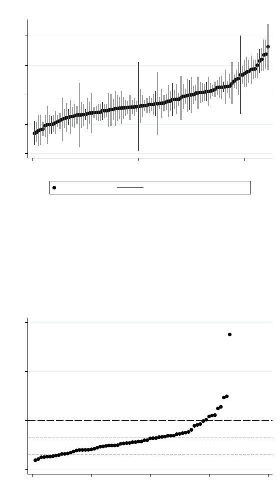
Figure 2: Predicted Nationwide Eﬀects by Site

0 1 2 3 4

First−Year Electricity Cost Savings ($ billions)

0 50 100

Site

Point Estimate 90 Percent Confidence Interval

Predicted National Effects by Site

Notes: This ﬁgure presents the national electricity cost savings that would be predicted by extrapolating

the ATE from the ﬁrst year of each existing Opower site to all US households.

Figure 3: Cost Eﬀectiveness by Site

Friedrich et al. lower bound

Friedrich et al. upper bound

Arimura et al. estimate

0 5 10 15

Cost Effectiveness (cents/kWh)

0 20 40 60 80

Site

Two−Year Cost Effectiveness by Site

Notes: This ﬁgure presents the cost eﬀectiveness over the ﬁrst two years of each program against national

benchmark estimates from Arimura et al. (2011) and Friedrich et al. (2009).

Figure 4: Predicted Eﬀects Using Microdata

ATE

Linear Fit

Weighted Fit

Linear Fit

Weighted Fit

True ATE

Microdata Nationwide Later Sites

0 .2 .4 .6 .8 1 1.2 1.4 1.6 1.8 2

Frequency−Adjusted ATE (Percent)

Out−of−Sample Prediction Using Microdata

Notes: This ﬁgure presents the eﬀects of the Opower program as predicted by microdata from the ﬁrst

ten sites. The left panel is the sample estimate, the middle panel is the nationwide prediction, and the right

panel is the prediction for the 101 later sites that are in the metadata but not the microdata. The “True

ATE” is the actual average ATE for the later sites.

Figure 5: Eﬃcacy Trend

0 .5 1 1.5 2 2.5

Frequency−Adjusted ATE (Percent)

1/2008 1/2009 1/2010 1/2011 1/2012 1/2013

Wave Start Date

ATE Linear Trend

Efficacy by Start Date

Notes: This ﬁgure plots the data and ﬁtted regression line matching column 1 of Table 7.

Figure 6a: States with Opower Sites

Notes: Shaded states have an Opower site. Darker colors indicate earlier program start dates.

Figure 6b: States with Energy Eﬃciency Resource Standards and Agencies

Notes: Shaded states have either a quasi-governmental energy eﬃciency agency (Maine, Vermont, Ore-

gon, and Hawaii) or an Energy Eﬃciency Resource Standard.

Figure 6c: State Hybrid Vehicle Shares

Notes: Darker shading represents a higher ratio of hybrid vehicles to total vehicles registered as of 2013.

Figure 6d: State Average Residential Electricity Usage

Notes: Darker shading indicates higher average residential electricity usage.

Figure 7: Within-Utility Eﬃcacy Trend

−1 −.5 0 .5

Frequency−Adjusted ATE (Percent)

−4 −2 0 2 4

Within−Utility Start Number

coef = −.0910693, (robust) se = .03884274, t = −2.34

Within−Utility Efficacy Trend

Notes: This ﬁgure plots the association between frequency-adjusted ATE and the within-utility start

number, conditional on utility ﬁxed eﬀects. This matches column 3 of Table 7. In estimating the best ﬁt

line, observations are weighted by inverse variance.

Figure 8: Site Selection on Population Preferences

.5 1 1.5 2 2.5

Frequency−Adjusted ATE (Percent)

.2 .4 .6 .8 1

Population Preferences Mechanism Score

Population Preferences Site Selection Mechanism

Notes: This ﬁgure plots the regression of frequency-adjusted ATE on the population preferences mecha-

nism score, which is based oﬀ of Income, Share College Grads, Hybrid Share, Democratic Vote Share, Green

Vote Share, Energy Eﬃciency Resource Standard, and Green Pricing Market Share. The solid line is the best

ﬁt line, and the dashed line is the best ﬁt line excluding the four outlying points to the left. In estimating

the best ﬁt lines, observations are weighted by inverse variance.

Appendix: For Online Publication

Site Selection Bias in Program Evaluation

Hunt Allcott

Appendix I: Correlations with Democratic Vote Share

Political aﬃliation provides an interesting case study of diﬃculties in estimating interaction eﬀects in mi-

crodata. In my ten-site microdata sample, the association between the treatment eﬀect and Census tract

Democratic vote share is not robust and is often negative.

A negative association is both counter to other

correlations between political aﬃliation and measures of environmentalism and also counter to the correla-

tion in my site-level metadata. Here I show that the lack of robustness in microdata is due to the correlation

between Democratic vote share and other X covariates, and “unexpected” negative associations can result

because these correlations have diﬀerent signs within cities vs. across counties.

Across counties in the U.S., Democratic vote shares are positively associated with socioeconomic status

(SES), as measured by variables such as income and education. Across Census tracts within Opower samples,

however, Democratic vote share is negatively associated with SES. As shown in Appendix I Table AI-1,

Democratic Census tracts within cities use less electricity and are more urban, with lower income, less

education, fewer single-family homes, and more renters. Furthermore, the empirical association between

measures of environmentalism and political ideology is not straightforward: households in Democratic Census

tracts are more likely to participate in green pricing programs, but they are less likely to participate in the

utility’s other energy eﬃciency programs, conditional on income and education. Columns 6 and 7 restrict to

Census tracts in site 10 because Green Pricing and EE Program Participant are only observed in that site.

I observe households’ Census block group in site 10 (only), and the results in column 6 and 7 are similar

using block group-level data.

Appendix I Table AI-2 illustrates the problems that these associations can generate when trying to

estimate an α for Democratic vote share. Columns 1-3 show that Democratic neighborhoods have smaller

treatment eﬀects, both conditional on all other covariates and unconditional. However, simply controlling

for the interaction between T and Y

in column 4 eliminates this negative association. In columns 5 and 6,

I limit the sample to Site 10 and use the block-group level Democratic vote shares. Column 5 replicates the

approach in column 2, showing a negative but highly insigniﬁcant association. However, when I use ln Y as

the outcome variable (multiplying by 100 to make the coeﬃcients comparable) and condition on interactions

between T and a particular set of other X variables, I can obtain a positive association between Democratic

vote share and the treatment eﬀect.

Because this association is both not robust in my data and potentially inconsistent with the site-level

comparative static, I do not attempt to extrapolate on Democratic vote share.

Costa and Kahn (2013) show that the share of Democratic voters in a household’s Census block group is positively

associated with the treatment eﬀect in one Opower site, conditional on interactions between T and other X covariates.

Their speciﬁcation and available covariates diﬀer from mine, and so this appendix is absolutely not a comment on

their results. They present a series of regressions showing that their results are robust in their speciﬁcations at their

site.

Appendix I Table AI-1: Associations with Democratic Vote Share

Baseline College Single Green EE Prog.

Dependent Variable: Usage Income Grads Family Rent Pricing Participant

(1) (2) (3) (4) (5) (6) (7)

Democratic Vote Share -14.475 -134.747 -0.367 -1.196 0.665 0.076 -0.051

(5.097)** (13.947)*** (0.111)*** (0.074)*** (0.073)*** (0.044)* (0.014)***

Income -0.001 -0.000

(0.000)* (0.000)

Share College Grads 0.209 0.042

(0.036)*** (0.015)***

0.11 0.28 0.06 0.32 0.25 0.51 0.26

Within R2 0.11 0.28 0.06 0.32 0.25

Between R2 0.01 0.00 0.33 0.79 0.06

N 1,386 1,385 1,385 715 1,117 85 85

Notes: This table presents associations between Democratic vote share and various other variables, using

data collapsed to Census tract-level averages. Columns 1-5 include all 10 microdata sites, while columns 6-7

include only site 10. *, **, ***: Statistically signiﬁcant with 90, 95, and 99 percent conﬁdence, respectively.

Appendix I Table AI-2: Estimates Including Democratic Vote Share

(1) (2) (3) (4) (5) (6)

Treatment 1.730 2.137 1.967

(0.055)*** (0.157)*** (0.225)***

T x Democratic Vote Share -2.190 -1.503 -1.609 -0.318 -0.696 2.773

(0.655)*** (0.717)** (0.583)*** (0.600) (1.448) (1.512)*

T x First Comparison 0.097 0.097 0.175

(0.010)*** (0.010)*** (0.020)***

T x Income -0.001 0.001 0.010

(0.004) (0.004) (0.012)

T x Share College Grads 0.305 -0.199 -2.014 0.113

(0.702) (0.780) (1.790) (1.123)

T x Hybrid Share 2.775 11.984 9.341

(8.538) (10.443) (22.346)

T x Green Pricing 0.172 0.197 0.250

(0.332) (0.334) (0.331)

T x EE Program Participant 0.048 0.021 0.052

(0.391) (0.388) (0.386)

T x Electric Heat 1.397 1.255 1.663

(0.265)*** (0.266)*** (0.426)***

T x HouseAge 0.003 0.001 0.004 -0.013

(0.002) (0.003) (0.011) (0.013)

T x Has Pool 1.150 1.068 0.831

(0.305)*** (0.312)*** (0.370)**

T x Rent -0.247 -0.273

(0.298) (0.305)

T x Single Family 0.589 0.544

(0.240)** (0.272)**

T x Square Feet 0.431 0.415 0.769

(0.120)*** (0.122)*** (0.360)**

T x Baseline Usage 0.069 0.029

(0.011)*** (0.013)**

R2 0.87 0.87 0.86 0.86 0.90 0.83

N 508,295 508,295 508,295 508,295 82,836 82,831

Sample Sites All All All All Site 10 Site 10

T x Site Indicators No Yes Yes Yes N/A N/A

Dependent Var: Y Y Y Y Y 100*ln(Y)

Notes: This table presents estimates of Equation (7) with diﬀerent X characteristics. The outcome

variable in columns 1-5 is Y

, household i’s post-treatment electricity use normalized by the site s control

group post-treatment average. In column 6, the outcome variable is 100 · ln Y

. Robust standard errors are

in parenthesis. *, **, ***: Statistically signiﬁcant with 90, 95, and 99 percent conﬁdence, respectively.

Appendix II: Site Selection Bias in Other Contexts

The Opower experiments provide one case study of site selection bias. This appendix explores the possibility

that site selection bias might exist in other contexts. The appendix begins with a discussion of site selection

mechanisms that could be relevant across a variety of domains. I then provide suggestive empirical evidence

from microﬁnance and clinical trials.

Site Selection Mechanisms

Site selection mechanisms could represent two situations. First, sites could represent potential program

implementation partners that would adopt a new program and evaluate it using a randomized trial. This

is the case with Opower, as they approach additional utilities about adopting their Home Energy Report

program. Second, sites could represent potential program evaluation partners that are already running an

existing program and must decide whether to use an RCT for impact evaluation. This was eventually the

case with the Job Training Partnership Act (JTPA) evaluations: the researchers approached existing JTPA

job training centers to recruit them to implement an RCT.

One natural way to model site selection mechanisms is through a Roy-like selection equation in which

decision makers at each potential partner site decide whether to adopt or evaluate a program based on

whether the costs outweigh the beneﬁts. Potential partner sites incur some positive or negative net cost C

of adopting or evaluating the treatment and weight average outcomes Y

by ω. The decision makers also

have some signal a

of the treatment eﬀect, with a

= τ

+ ν

, where the noise ν has mean zero and variance

. The potential partner site becomes an actual partner if perceived net beneﬁts are positive:

= 1 [ωa

− C

> 0] (12)

The generalized Roy model again highlights the close analogy to individual-level selection problems that

threaten internal validity. Under these site selection mechanisms, external unconfoundedness only holds only

if the selection process happens to be independent of unobservables. Otherwise, there is site selection bias.

Table AII-1 gives an example set of positive and negative site selection mechanisms that might be

relevant in diﬀerent settings. There are two classes of mechanisms through which ωa − C might depend

on Z

. One is driven by selection on gain: the mechanical correlation between ωa and Z

. If potential

partners care about outcomes when they decide whether to implement a new program or evaluate an existing

program, and if their signal a includes econometrically unobserved information Z

, then actual partners will

be selected on unobservables. One speciﬁc mechanism within this class is targeting gains: decision makers

at potential partner sites who think their populations would be more likely to beneﬁt from a new program

would be more likely to adopt it. Similarly, implementers such as Opower may want to immediately showcase

a new program’s eﬃcacy, giving them incentives to focus early partner recruitment on sites expected to

have particularly responsive populations. Population preferences is a related but diﬀerent mechanism: a

population of individuals could perceive local beneﬁts and encourage the site-level decision maker to adopt

a program. Opower provides a clear example, where populations in environmentalist states pass Energy

Eﬃciency Resource Standards that require utilities to adopt energy eﬃciency programs.

An additional related mechanism results from the fact that it pays to be ignorant, as argued by Pritchett

(2002). Because rigorous evaluations are publicized and aﬀect funding from foundations and governments,

potential partners whose signals suggest that their existing programs are eﬀective may be more willing to

have them rigorously evaluated, while those that believe they are running ineﬀective programs strategically

choose to avoid RCTs. The cost of RCTs plus imperfect information about other dimensions of program

quality keep this equilibrium from unraveling into an equilibrium in which RCTs are run at all sites.

The second class of mechanisms is driven by selection on net cost: the potential correlation between C

and Z

. A site-level form of ability bias results from the fact that implementing randomized trials requires

managerial ability and operational eﬀectiveness. Potential partners that are most able to implement RCTs,

and thus have low C, also implement the treatment most eﬀectively. For example, Bold et al. (2013) show

that the NGO which had ﬁrst implemented a contract teacher RCT in Kenyan schools was much more

eﬀective at implementing the program, paying teachers on time, monitoring performance, and incentivizing

eﬀort than the Kenyan government, which was eventually responsible for scaling up the program. This form

of positive partner selection bias is related to the idea of “gold plating” (Duﬂo, Glennerster, and Kremer

2008): in order to cleanly measure eﬃcacy, treatments are often implemented with much greater precision

and quality in experimental settings than they would be elsewhere.

Many types of organizations run multiple programs: hospitals oﬀer a variety of patient services, utilities

run many diﬀerent energy eﬃciency programs, and social services centers might oﬀer health clinics, transla-

tion, and job training. Able, eﬀective, and innovative potential RCT partners may also oﬀer more or better

programs in addition to the intervention being evaluated. If there are complementary programs, then this

causes positive site selection bias. On the other hand, there could be substitute programs: multiple interven-

tions addressing the same outcomes, with diminishing returns to additional interventions. This would cause

negative site selection bias.

An additional mechanism generating negative site selection is targeting needs. This would occur if early

adopters of a new program target disadvantaged populations, but it is diﬃcult to implement the treatment in

areas where disadvantaged populations live. For example, Luoto and Levine (2013) evaluates an experiment

that used mobile payments to facilitate credit for water ﬁlter purchases. The experiment targeted rural parts

of a poor province in Kenya, where mobile payments are familiar but are not frequently used to pay bills.

As a result, takeup rates were lower than they might be in other parts of the country.

Microﬁnance

In the past ten years, there have been a large set of ﬁeld experiments with microﬁnance institutions (MFIs).

Do MFI partners diﬀer from non-partners on observables that could be correlated with treatment eﬀects? If

so, this suggests the possibility of site selection bias.

For both microﬁnance and clinical trials, I follow the same approach. First, I deﬁne a population

of potential partner sites. Second, I gather site-level observables that theory suggests could moderate the

eﬀects of diﬀerent interventions. Third, I compare sample to non-sample sites on these potential moderators.

Unlike with Opower, the interventions vary, so it is not possible to take the next step of correlating selection

probability with a consistently-deﬁned treatment eﬀect. Instead, this section is merely intended to brieﬂy

present suggestive evidence on whether site selection bias is unique to the Opower context.

I deﬁne the population of sites as all MFIs included in the Microﬁnance Information Exchange (MIX)

global database. The database includes information on the characteristics and performance of 1903 MFIs in

115 countries. Partners are deﬁned as all MFIs listed as RCT partners on the Jameel Poverty Action Lab,

Innovations for Poverty Action, and Financial Access Initiative websites. About two percent of MFIs in the

database are RCT partners. I focus on MFI characteristics that might theoretically be correlated with the

outcomes of diﬀerent ﬁeld experiments. Average loan balance, percent of portfolio at risk of default, and the

percent of borrowers who are female could be correlated with default rates, which are a common outcome

variable in microﬁnance RCTs. Just as in the Opower experiments, partner structure (as measured by age,

non-proﬁt status, and size) could inﬂuence the strength of the MFI’s relationship with its clients, which

might in turn aﬀect the MFI’s ability to implement or monitor an intervention. Similarly, staﬀ availability

and expenditures per borrower could aﬀect implementation or monitoring ability.

Table AII-2 presents the means and standard deviations of these characteristics by partner status. The

rightmost column presents diﬀerences in mean characteristics of partners vs. non-partners. Partners have

smaller average loan balances, as well as marginally insigniﬁcantly lower percent of portfolio at risk and more

female borrowers. Each of these factors could be associated with lower default rates, and because default

rates in many microﬁnance experiments are very low, it is possible that eﬀects of various treatments on

default rates would be larger against a larger baseline in non-partner MFIs. Partner MFIs are also older,

larger, and more likely to be for proﬁt, perhaps because RCTs require large samples and well-managed

partners. Finally, partner MFIs have statistically signiﬁcantly fewer staﬀ and lower costs per borrower.

Overall, partner MFIs diﬀer statistically on six of these eight individual characteristics, and an F-test of a

regression of partner status on all characteristics easily rejects the hypothesis that partners and non-partners

do not diﬀer on observables.

Clinical Trials

What types of hospitals carry out clinical trials for new drugs and procedures? If clinical trials are more

common at research hospitals with more urban patient populations, higher-ability doctors, and better medical

technologies, and if these factors moderate the eﬃcacy of medical interventions, this would suggest site

selection bias.

Wennberg et al. (1998) provide a motivating example. In the 1990s, there were two large trials that

tested carotid endarterectomy, a surgical procedure which treats hardening of the carotid artery in the neck.

In order to participate, institutions and surgeons had to be experienced in the procedure and have low

previous mortality rates. After the trials found the procedure to be preferred to alternative approaches,

its use nearly doubled. Wennberg et al. (1998) use a broader sample of administrative data to show that

mortality rates were signiﬁcantly higher at non-trial hospitals, and for some classes of patients and hospitals,

treatment with drugs instead of the surgical procedure might have been preferred.

The database for Aggregate Analysis of ClinicalTrials.gov (AACT) gives comprehensive information on

clinical trials registered in the oﬃcial database operated by the U.S. National Institute of Health. I separately

consider two types of clinical trials: “Drug” trials, which includes drugs, biological interventions, and dietary

supplements, and “Procedure” trials, which include both surgical and radiation procedures. The site names

and zip codes can be matched to the set of all hospitals in the U.S., which form the target population of

hospitals where the interventions will be implemented.

Table AII-3 compares characteristics of hospitals that have been the site of at least one clinical trial to

hospitals that have never hosted a registered trial. Hospital characteristics are drawn from the Medicare

Hospital Compare database, the American Hospital Association (AHA) Annual Survey, and the NBER

Medicare Provider of Services (POS) ﬁles. Appendix III presents more details on data preparation.

The ﬁrst three rows show that clinical trial sites are at hospitals in urban areas and in counties with

higher income and education. Remaining characteristics are grouped using the standard Donabedian’s (1988)

triad of clinical quality measures: structure, process, and outcomes.

Clinical trial sites have signiﬁcantly diﬀerent structures. They take place at hospitals that are signiﬁcantly

larger, in terms of both beds and admissions. Furthermore, trial site hospitals perform many more surgeries

per year. This is particularly important in light of evidence from Chandra and Staiger (2007), who show that

due to productivity spillovers, surgical interventions are more eﬀective in areas that perform more surgeries.

In their conclusion, Chandra and Staiger (2007) point out that this may compromise the external validity of

randomized control trials.

Clinical trial site hospitals are much more likely to have adopted electronic medical records, and the

average site has ﬁve to six more of the 21 advanced technologies identiﬁed by US News in their Hospital

Quality Rankings. Trial sites also oﬀer an average of three more of the 13 patient services scored by US

News. If these technologies and services are complements to surgical and radiation procedures, or perhaps

even to drugs, then these interventions will be less eﬀective at non-trial sites.

Clinical trial sites also diﬀer in the processes they use. They perform 0.33 to 0.35 standard deviations

better on ﬁve surgical process measures included in the Hospital Safety Score (HSS) methodology. If sur-

geons’ adherence to accepted procedures is associated with better outcomes, surgical procedures will tend

to be more eﬀective at trial hospitals compared to non-trial hospitals. On the other hand, patient sur-

veys show that doctors and nurses at trial site hospitals are worse at communication, including explaining

medicines and what to do during recovery. Because patients’ understanding of how to take a drug might

aﬀect adherence, and understanding of what to do during recovery might aﬀect how well people recover from

surgical procedures, eﬀects of drugs and procedures could be worse through this channel at trial vs. non-trial

hospitals.

The next four measures in the table capture outcomes. The measures are only slightly correlated, usually

with correlation coeﬃcients under 0.1, which likely reﬂects some combination of measurement error and true

independence in the data. Clinical trial sites perform worse on two outcome measures: they have 0.13 to

0.14 standard deviations higher rates of four hospital-acquired conditions included in the HSS, and 0.21 to

0.25 standard deviations higher rates of six complications included in the HSS patient safety indicator index.

Clinical trial sites do not diﬀer on the rate of infections during colon surgery, and they have substantially

lower mortality rates when treating patients suﬀering from heart attack, heart failure, and pneumonia.

Finally, clinical trial sites are 4 to 7 percentage points more likely to appear in the top 50 hospitals in

12 specialties rated by the US News Hospital Quality Rankings, and they have an average of 0.17 to 0.29

additional specialties ranked. Against a small base, these diﬀerences are very large in percent terms. Overall,

these results point to “ability bias” as a site selection mechanism in clinical trials: almost mechanically,

clinical trials take place at higher-quality hospitals because technology, size, and skill are complements to

clinical research.

Appendix II Table AII-1: Example Site Selection Mechanisms

Selection Mechanism Sign Example

Selection on Gain:

Targeting Gains Positive Implementers target most responsive populations.

Population Preferences Positive Responsive populations encourage partners to adopt.

It Pays to Be Ignorant Positive Partners with ineﬀective programs do not want to evaluate.

Selection on Net Cost:

Ability Bias Positive RCTs require operational ability; ability also increases eﬃcacy.

Complementary Programs Positive Able and eﬀective partners also oﬀer complementary programs.

Substitute Programs Negative Able and eﬀective partners have other substitute programs,

and the marginal intervention has lower returns.

Targeting Needs Negative Implementers target the neediest populations, which are hardest to reach.

Appendix II Table AII-2: MFI Site Characteristics

All Partners Non-Partners Diﬀerence

Average Loan Balance ($000’s) 1.42 0.58 1.44 -0.86

(3.07) (0.51) (3.10) (0.12)

∗∗∗

Percent Portfolio at Risk 0.083 0.068 0.083 -0.015

(0.120) (0.066) (0.121) (0.012)

Percent Women Borrowers 0.62 0.69 0.62 0.07

(0.27) (0.27) (0.27) (0.05)

MFI Age (Years) 13.99 21.86 13.84 8.02

(10.43) (11.21) (10.36) (1.88)

∗∗∗

Non-Proﬁt 0.63 0.37 0.64 -0.27

(0.48) (0.49) (0.48) (0.08)

∗∗∗

Number of Borrowers (10

) 0.06 0.85 0.05 0.80

(0.40) (1.84) (0.27) (0.31)

∗∗∗

Borrowers/Staﬀ Ratio (10

) 0.13 0.22 0.13 0.09

(0.21) (0.19) (0.21) (0.03)

∗∗∗

Cost per Borrower ($000’s) 0.18 0.10 0.18 -0.08

(0.19) (0.08) (0.19) (0.01)

∗∗∗

N 1903 35 1868

F Test p-Value 0.00002

∗∗∗

Notes: The ﬁrst three columns present the mean characteristics for all MFIs, for ﬁeld experiment partners,

and for ﬁeld experiment non-partners, respectively. Standard deviations are in parenthesis. The fourth

column presents the diﬀerence in means between partners and non-partners, with robust standard errors

in parenthesis. *, **, ***: Statistically signiﬁcant with 90, 95, and 99 percent conﬁdence, respectively.

Currencies are in US dollars at market exchange rates. Percent of Portfolio at Risk is the percent of gross

loan portfolio that is renegotiated or overdue by more than 30 days.

Appendix II Table AII-3: Clinical Trial Site Characteristics

Population Drug Trials Procedure Trials

Mean Diﬀerence Diﬀerence

County Percent with College Degree 0.23 0.09 0.08

(0.10) (0.00)

∗∗∗

(0.00)

∗∗∗

County Income per Capita 37.6 7.7 7.4

(10.7) (0.3)

∗∗∗

(0.4)

∗∗∗

Urban 0.57 0.47 0.42

(0.49) (0.01)

∗∗∗

(0.01)

∗∗∗

Bed Count 179 238 256

(214) (7)

∗∗∗

(8)

∗∗∗

Annual Number of Admissions (000s) 7.4 11.0 11.9

(9.6) (0.3)

∗∗∗

(0.4)

∗∗∗

Annual Number of Surgeries (000s) 5.8 8.0 8.7

(7.5) (0.2)

∗∗∗

(0.3)

∗∗∗

Uses Electronic Medical Records 0.62 0.13 0.15

(0.31) (0.01)

∗∗∗

(0.01)

∗∗∗

US News Technology Score 4.92 5.27 5.75

(4.78) (0.14)

∗∗∗

(0.16)

∗∗∗

US News Patient Services Score 4.42 2.87 3.16

(3.16) (0.09)

∗∗∗

(0.10)

∗∗∗

Surgical Care Process Score 0.00 0.35 0.33

(1.00) (0.03)

∗∗∗

(0.03)

∗∗∗

Patient Communication Score 0.00 -0.36 -0.23

(1.00) (0.03)

∗∗∗

(0.03)

∗∗∗

Hospital-Acquired Condition Score 0.00 0.13 0.14

(1.00) (0.03)

∗∗∗

(0.03)

∗∗∗

Patient Safety Indicator Score 0.00 0.21 0.25

(1.00) (0.03)

∗∗∗

(0.04)

∗∗∗

Surgical Site Infection Ratio: Colon 0.00 -0.02 0.03

(1.00) (0.06) (0.05)

Mortality Rate Score 0.00 -0.34 -0.37

(1.00) (0.03)

∗∗∗

(0.03)

∗∗∗

US News Top Hospital 0.04 0.04 0.07

(0.21) (0.01)

∗∗∗

(0.01)

∗∗∗

Specialties in US News Top 50 0.20 0.17 0.29

(1.25) (0.04)

∗∗∗

(0.05)

∗∗∗

N 4653

F Test p-Value 0.0000

∗∗∗

0.0000

∗∗∗

Notes: The ﬁrst column presents the mean characteristic for all US hospitals, with standard deviations

in parenthesis. The second and third columns present diﬀerences in means between trial sample sites and

non-sample sites, with robust standard errors in parenthesis. *, **, ***: Statistically signiﬁcant with 90, 95,

and 99 percent conﬁdence, respectively.

Appendix III: Preparation of Clinical Trial and Hospital Data in

Appendix II

ClinicalTrials.gov is a registry and results database of clinical trials conducted in the United States and

other countries. Although the registry does not contain all clinical studies, the number of studies registered

has increased as policies and laws requiring registration have been enacted and as voluntary registration has

caught on. The database for Aggregate Analysis of ClinicalTrials.gov contains records of each registered trial

as of September 27, 2012 (CTTI 2012). There were 108,047 “interventional” studies (randomized control

trials). Of these, 71 percent were “Drug trials,” by which I mean that at least one treatment group was

given a drug, biological intervention, or dietary supplement. Thirteen percent were “Procedure trials,” by

which I mean that at least one treatment group received a surgical or radiation procedure. Each trial takes

place at one or more sites, and there are 480,000 trial-by-site observations for Drug trials and 72,000 trial-

by-site observations for Procedure trials. Many trials take place at clinics, corporate research sites, or other

institutions: 135,000 and 37,000 trial-by-site observations of Drug and Procedure trials, respectively, were

matched to the hospital database using hospital name and zip code.

The hospital database combines three major data sources: the NBER Center for Medicare & Medicaid

Services (CMS) Provider of Services (POS) ﬁles for 2011 (NBER 2013), the American Hospital Association

(AHA) Annual Survey Database for 2011 (AHA 2012), and the CMS Hospital Compare database (CMS

2013). Hospitals are linked between the databases using the six-digit CMS provider identiﬁcation number.

From the POS ﬁles, I extract the hospital name, county, zip code, urban location indicator variable, and bed

count.

From the AHA database, I extract number of admissions and number of surgical procedures, as well as

information on electronic medical records and the US News Technology and Patient Services scores. The

Electronic Medical Records variable takes value 1 if the hospital has fully implemented, 0.5 if partially

implemented, and zero if there are no electronic medical records. In their Best Hospitals 2013-2014 rankings,

U.S. News and World Report identiﬁes 21 technologies as part of their Index of Hospital Quality (U.S. News

2013), from ablation of Barrett’s esophagus to transplant services. The U.S. News Technology Score variable

is simply the number of these technologies that the hospital oﬀers on-site. U.S. News also identiﬁes 13 patient

services, from an Alzheimer’s center to wound management services. Analogously, the U.S. News Patient

Services Score is the number of these services that the hospital oﬀers on-site.

The remainder of the measures are from the CMS Hospital Compare database. Each of the measures

described below is normalized across hospitals to mean zero, standard deviation one. The Patient Commu-

nication Score combines four variables from the Survey of Patients’ Hospital Experiences using the following

formula:

Percent of patients who reported that their nurses ”Always” communicated well

· Percent of patients who reported that their nurses ”Usually” communicated well

Percent of patients who reported that their doctors ”Always” communicated well

· Percent of patients who reported that their doctors ”Usually” communicated well

+Percent of patients who reported that staﬀ ”Always” explained about medicines

· Percent of patients who reported that staﬀ ”Usually” explained about medicines

+Percent of patients who reported that YES they were given

information about what to do during recovery

The Mortality Rate Score variable is the sum of three components: the 30-day mortality rates from

pneumonia, heart failure, and heart attack. Each component is normalized to mean zero, standard deviation

one before being added together.

The next four variables from Hospital Compare were motivated directly from the Hospital Safety Score

methodology, available from http://www.hospitalsafetyscore.org. The Surgical Care Process Score is the

sum of ﬁve measures from the Surgical Care Improvement Project, which reports the percentage of times

that surgeons at the hospital followed accepted practices, from giving prophylactic antibiotic within one hour

of surgical incision to giving appropriate venous thromboembolism. For each of the ﬁve speciﬁc measures, I

normalized the percentages to have mean zero, standard deviation one across hospitals so as to not overweight

variation coming from any one measure. I then summed the normalized measures and again normalized the

sum to have mean zero, standard deviation one.

The Surgical Site Infection Ratio is the Standardized Infection Ratio for Colorectal Surgery.

The Hospital Safety Score includes the incidence rates of four Hospital Acquired Conditions: foreign

object retained after surgery, air embolism, pressure ulcers, and falls and trauma. Each of these individual

rates is normalized to mean zero, standard deviation one. The Hospital Acquired Condition Score is the sum

of these four normalized measures.

The Hospital Safety Score incorporates six measures from the Agency for Healthcare Research and

Quality Patient Safety Indicators (PSIs), which are again reported as incidence rates. These include sur-

gical deaths, collapsed lungs, post-operative blood clots, post-operative ruptured wounds, and accidental

lacerations.

Appendix IV: Additional Tables and Figures Referenced in Body

of Paper

Appendix Table A1: Household Characteristics by Site

Energy Census

Use Tract Household

Baseline First Mean Share Hybrid EE House

Site Usage Comparison Income College Vehicle Green Program Electric Age Has Single Square

Number (kWh/day) (kWh/day) ($000s) Grads Share Pricing Participant Heat (Years) Pool Rental Family Feet (000s)

1 30.9 3.33 89.9 0.40 0.013 - - - 50.3 - 0.09 0.77 1.91

(5.7) (14.6) (41.0) (0.21) (0.009) - - - (26.1) - (0.29) (0.42) (0.90)

2 29.7 0.00 70.2 0.21 0.007 - - 0.08 31.7 - - 0.96 1.69

(16.4) (18.5) (12.9) (0.08) (0.003) - - (0.27) (28.1) - - (0.21) (0.54)

3 25.1 0.37 62.9 0.47 0.018 - - 0.14 25.5 - 0.32 0.74 2.01

(13.2) (11.1) (18.8) (0.11) (0.007) - - (0.35) (20.6) - (0.47) (0.44) (0.78)

4 18.2 1.33 63.7 0.34 0.022 - - - 59.2 0.10 0.35 0.50 1.69

(10.7) (9.9) (27.5) (0.11) (0.009) - - - (23.1) (0.30) (0.48) (0.50) (0.72)

5 39.5 -2.45 45.3 0.16 0.004 - - 0.31 - - 0.05 - 1.28

(27.5) (24.2) (6.0) (0.05) (0.002) - - (0.46) - - (0.21) - (0.54)

6 30.0 2.49 82.5 0.39 0.013 - - - 58.6 0.02 0.06 - 2.03

(14.8) (13.3) (30.0) (0.16) (0.006) - - - (42.4) (0.15) (0.23) - (0.85)

7 30.5 2.88 85.4 0.40 0.024 - - 0.07 31.0 - 0.03 - 2.14

(13.8) (15.4) (30.7) (0.16) (0.012) - - (0.26) (16.0) - (0.18) - (0.64)

8 31.2 -1.13 65.3 0.25 0.019 - - - 28.0 0.24 - 0.62 1.88

(22.5) (13.9) (31.2) (0.09) (0.008) - - - (15.7) (0.43) - (0.49) (0.80)

9 36.4 3.48 70.6 0.47 0.035 - - 0.17 65.0 - 0.06 - 1.83

(17.2) (16.3) (23.1) (0.18) (0.015) - - (0.38) (25.4) - (0.23) - (0.77)

10 30.8 0.98 70.9 0.36 0.020 0.09 0.06 0.25 37.4 0.21 - - 1.75

(15.1) (14.1) (17.2) (0.14) (0.010) (0.29) (0.24) (0.44) (18.3) (0.41) - - (0.60)

Notes: This table presents the means of household characteristics for each of the ten initial Opower sites, with standard deviations in

parenthesis. A dash means that a variable is not observed at that site.

Appendix Table A2: Adjustment for Treatment Frequency

Site 2 Site 7 Both

(1) (2) (3)

T x Reports/Month 0.489 0.554 0.517

(0.283)* (0.309)* (0.209)**

Treatment x Site 2 1.465 1.445

(0.248)*** (0.204)***

Treatment x Site 7 1.071 1.101

(0.279)*** (0.209)***

R2 0.89 0.86 0.88

N 72,687 78,549 151,236

T x Site Indicators N/A N/A Yes

Notes: This table presents estimates of the frequency adjustment parameter used in Equation (2). The

estimating equation is Equation (7), using the number of reports per month as the only X characteristic.

The outcome variable is Y

, household i’s post-treatment electricity use normalized by the site s control

group post-treatment average. Robust standard errors are in parenthesis. *, **, ***: Statistically signiﬁcant

with 90, 95, and 99 percent conﬁdence, respectively.

Appendix Table A3: Site-Speciﬁc Heterogeneous Eﬀects

Site: (1) (2) (3) (4) (5) (6) (7) (8) (9) (10)

Treatment 1.325 1.789 1.901 2.039 2.539 1.567 1.537 1.123 1.628 2.187

(0.154)*** (0.131)*** (0.236)*** (0.208)*** (0.338)*** (0.142)*** (0.122)*** (0.277)*** (0.200)*** (0.138)***

T x First Comparison 0.014 0.090 0.038 0.100 0.102 0.055 0.112 -0.034 0.285 0.172

(0.020) (0.016)*** (0.044) (0.050)** (0.022)*** (0.022)** (0.015)*** (0.091) (0.059)*** (0.019)***

T x Income -0.006 0.036 0.032 0.067 -0.078 0.004 -0.002 0.025 0.015 0.016

(0.007) (0.014)*** (0.024) (0.024)*** (0.076) (0.013) (0.008) (0.016) (0.015) (0.015)

T x Share College Grads -1.482 2.855 2.329 -7.540 12.684 -2.261 -0.404 -9.925 0.254 -4.011

(1.682) (2.953) (4.004) (4.864) (8.815) (2.908) (1.852) (5.823)* (2.181) (1.798)**

T x Hybrid Share 79.237 -115.407 -104.139 -96.243 -36.715 70.936 -8.543 37.041 13.273 24.805

(29.782)*** (74.025) (60.441)* (62.623) (223.038) (47.497) (26.372) (63.000) (28.724) (22.212)

T x HouseAge 0.000 0.006 0.017 0.005 -0.008 -0.006 -0.037 0.005 0.003

(0.010) (0.005) (0.022) (0.015) (0.004)* (0.009) (0.030) (0.009) (0.012)

T x Rent 0.498 0.052 -1.280 1.128 -1.306 0.294 -1.671

(0.755) (0.702) (0.665)* (1.707) (0.760)* (0.999) (1.171)

T x Single Family -0.012 1.431 1.584 -0.268 0.222

(0.502) (0.493)*** (0.818)* (0.722) (0.641)

T x Square Feet 0.190 0.031 0.670 0.695 1.637 0.031 0.587 -0.300 0.425 0.847

(0.348) (0.345) (0.410) (0.718) (1.815) (0.273) (0.257)** (0.999) (0.335) (0.327)**

T x Electric Heat -2.812 2.695 2.439 0.931 1.227 1.539

(0.999)*** (1.367)** (0.911)*** (0.565)* (0.658)* (0.420)***

T x Has Pool 2.393 0.315 1.348 0.864

(1.014)** (0.923) (1.147) (0.378)**

T x Green Pricing 0.243

(0.333)

T x EE Program Participant 0.049

(0.393)

R2 0.50 0.90 0.83 0.92 0.89 0.90 0.86 0.89 0.83 0.90

N 54,259 72,687 38,502 33,308 17,558 49,165 78,549 42,576 38,855 82,836

Notes: This table presents estimates of Equation (7) for each speciﬁc site in the microdata. The outcome variable is Y

, household i’s

post-treatment electricity use normalized by the site s control group post-treatment average. Robust standard errors are in parenthesis. *,

**, ***: Statistically signiﬁcant with 90, 95, and 99 percent conﬁdence, respectively.

Appendix Table A4: Empirical Likelihood Results for Re-Weighting Estimator

Target: National Later Sites

(1) (2)

First Comparison 0.004 0.001

(0.000)*** (0.000)***

Electric Heat -0.787 -0.605

(0.006)*** (0.006)***

Has Pool -0.171 -0.170

(0.011)*** (0.011)***

Single Family 0.467 0.525

(0.007)*** (0.008)***

Square Feet -0.004 0.064

(0.002) (0.005)***

Missing(First Comparison) 0.083 0.064

(0.011)*** (0.012)***

Missing(Electric Heat) -0.022 0.003

(0.008)*** (0.008)

Missing(Has Pool) -0.111 -0.112

(0.007)*** (0.007)***

Missing(Single Family) 0.031 0.047

(0.006)*** (0.007)***

Missing(Square Feet) 0.132 0.143

(0.006)*** (0.007)***

ln(Likelihood) 10,045.93 6,356.32

Notes: This table presents the empirical likelihood results used to re-weight the microdata. Column 1

presents the estimates to match national average characteristics, while column 2 presents estimates to match

the average characteristics in the 101 later sites.

Appendix Table A5: Correlations with Mechanism Scores

Usage Preferences Programs Structure

(1) (2) (3) (4)

Correlations with Selection

Partner -1.32 0.25 1.61 0.46

(0.22)

∗∗∗

(0.03)

∗∗∗

(0.16)

∗∗∗

(0.03)

∗∗∗

Utility Start Date (Years) 17.6 -2.9 -6.1 1.3

(4.2)

∗∗∗

(1.2)

∗∗

(1.5)

∗∗∗

(1.0)

Correlations with Covariates 0.0384

Utility Mean Usage (kWh/day) -

Income ($000s) 0.131

(0.007)

∗∗∗

Share College Grads 0.109

(0.008)

∗∗∗

Hybrid Share 0.152

(0.008)

∗∗∗

Democrat Vote Share 0.147

(0.009)

∗∗∗

Green Vote Share 0.069

(0.008)

∗∗∗

Energy Eﬃciency Resource Standard 0.257

(0.003)

∗∗∗

Green Pricing Market Share 0.051

(0.010)

∗∗∗

Residential Conservation/Sales 0.042

(0.004)

∗∗∗

Conservation Cost/Total Revenues 0.05

(0.002)

∗∗∗

Municipality-Owned Utility 0.054

(0.006)

∗∗∗

Investor-Owned Utility 0.17

(0.01)

∗∗∗

ln(Residential Customers) 0.20

(0.004)

∗∗∗

Electricity Price (cents/kWh)

Notes: This table presents unconditional correlations with mechanism propensity scores. The top panel

presents coeﬃcients from regressing partner status or the utility start date on the mechanism propensity

score. The bottom panel presents coeﬃcients from regressing the mechanism propensity scores individually

on each of their constituent variables Z

. Robust standard errors are in parenthesis. *, **, ***: Statistically

signiﬁcant with 90, 95, and 99 percent conﬁdence, respectively.

Appendix Table A6: Random Eﬀects Meta-Regression

(1) (2) (3) (4) (5) (6)

Utility Start Date (Years) -0.208 -0.142 -0.081

(0.030)*** (0.029)*** (0.037)**

Within-Utility Start Number -0.125 -0.088 -0.128 -0.083 -0.039

(0.029)*** (0.029)*** (0.027)*** (0.035)** (0.046)

Usage P-Score -2.525 -1.686 -3.242

(1.417)* (1.287) (1.390)**

Preferences P-Score 1.255 1.001 0.898

(0.298)*** (0.270)*** (0.262)***

Programs P-Score 0.513 0.312 0.744

(0.319) (0.288) (0.436)*

Structure P-Score -0.984 -0.732 -0.836

(0.342)*** (0.315)** (0.327)**

Site P-Score 0.358 0.667

(0.159)** (0.210)***

F 25.36 12.29 16.49 16.09 3.68 5.26

I2 0.80 0.79 0.74 0.71 0.85 0.89

N 111 111 111 66 111 111

Notes: This table presents estimates of Equation (11). The outcome variable is frequency-adjusted

ATE. This matches Table 8, except that it is estimated using random eﬀects meta-regression. Robust

standard errors are in parenthesis. *, **, ***: Statistically signiﬁcant with 90, 95, and 99 percent conﬁdence,

respectively.

Appendix Figure A1: ATEs vs. Frequency-Adjusted ATEs

.5 1 1.5 2 2.5

Frequency−Adjusted ATE (Percent)

.5 1 1.5 2 2.5

ATE (Percent)

ATE vs. Frequency−Adjusted ATE

Notes: This ﬁgure presents ATEs vs. frequency-adjusted ATEs. ATEs are ﬁtted to the average frequency

across the 111 sites using Equation (2), with parameter estimated in Appendix Table A2.