UNDERSTANDING VARIATION IN PARTITION COEFFICIENT, Kd

United States Office of Air and Radiation EPA 402-R-99-004A

Environmental Protection August 1999

Agency

UNDERSTANDING VARIATION IN

PARTITION COEFFICIENT, K

, VALUES

Volume I:

The K

Model, Methods of Measurement, and

Application of Chemical Reaction Codes

UNDERSTANDING VARIATION IN

PARTITION COEFFICIENT, K

, VALUES

Volume I:

The K

Model, Methods of Measurement, and

Application of Chemical Reaction Codes

August 1999

A Cooperative Effort By:

Office of Radiation and Indoor Air

Office of Solid Waste and Emergency Response

U.S. Environmental Protection Agency

Washington, DC 20460

Office of Environmental Restoration

U.S. Department of Energy

Washington, DC 20585

NOTICE

The following two-volume report is intended solely as guidance to EPA and other

environmental professionals. This document does not constitute rulemaking by the Agency, and

cannot be relied on to create a substantive or procedural right enforceable by any party in

litigation with the United States. EPA may take action that is at variance with the information,

policies, and procedures in this document and may change them at any time without public notice.

Reference herein to any specific commercial products, process, or service by trade name,

trademark, manufacturer, or otherwise, does not necessarily constitute or imply its endorsement,

recommendation, or favoring by the United States Government.

iii

FOREWORD

Understanding the long-term behavior of contaminants in the subsurface is becoming

increasingly more important as the nation addresses groundwater contamination. Groundwater

contamination is a national concern as about 50 percent of the United States population receives

its drinking water from groundwater. It is the goal of the Environmental Protection Agency

(EPA) to prevent adverse effects to human health and the environment and to protect the

environmental integrity of the nation’s groundwater.

Once groundwater is contaminated, it is important to understand how the contaminant

moves in the subsurface environment. Proper understanding of the contaminant fate and transport

is necessary in order to characterize the risks associated with the contamination and to develop,

when necessary, emergency or remedial action plans. The parameter known as the partition (or

distribution) coefficient (K

) is one of the most important parameters used in estimating the

migration potential of contaminants present in aqueous solutions in contact with surface,

subsurface and suspended solids.

This two-volume report describes: (1) the conceptualization, measurement, and use of the

partition coefficient parameter; and (2) the geochemical aqueous solution and sorbent properties

that are most important in controlling adsorption/retardation behavior of selected contaminants.

Volume I of this document focuses on providing EPA and other environmental remediation

professionals with a reasoned and documented discussion of the major issues related to the

selection and measurement of the partition coefficient for a select group of contaminants. The

selected contaminants investigated in this two-volume document include: chromium, cadmium,

cesium, lead, plutonium, radon, strontium, thorium, tritium (

H), and uranium. This two-volume

report also addresses a void that has existed on this subject in both this Agency and in the user

community.

It is important to note that soil scientists and geochemists knowledgeable of sorption

processes in natural environments have long known that generic or default partition coefficient

values found in the literature can result in significant errors when used to predict the absolute

impacts of contaminant migration or site-remediation options. Accordingly, one of the major

recommendations of this report is that for site-specific calculations, partition coefficient values

measured at site-specific conditions are absolutely essential.

For those cases when the partition coefficient parameter is not or cannot be measured,

Volume II of this document: (1) provides a “thumb-nail sketch” of the key geochemical processes

affecting the sorption of the selected contaminants; (2) provides references to related key

experimental and review articles for further reading; (3) identifies the important aqueous- and

solid-phase parameters controlling the sorption of these contaminants in the subsurface

environment under oxidizing conditions; and (4) identifies, when possible, minimum and

maximum conservative partition coefficient values for each contaminant as a function of the key

geochemical processes affecting their sorption.

This publication is the result of a cooperative effort between the EPA Office of Radiation

and Indoor Air, Office of Solid Waste and Emergency Response, and the Department of Energy

Office of Environmental Restoration (EM-40). In addition, this publication is produced as part of

ORIA’s long-term strategic plan to assist in the remediation of contaminated sites. It is published

and made available to assist all environmental remediation professionals in the cleanup of

groundwater sources all over the United States.

Stephen D. Page, Director

Office of Radiation and Indoor Air

ACKNOWLEDGMENTS

Ronald G. Wilhelm from ORIA’s Center for Remediation Technology and Tools was the

project lead and EPA Project Officer for this two-volume report. Paul Beam, Environmental

Restoration Program (EM-40), was the project lead and sponsor for the Department of Energy

(DOE). Project support was provided by both DOE/EM-40 and EPA’s Office of Remedial and

Emergency Response (OERR).

EPA/ORIA wishes to thank the following people for their assistance and technical review

comments on various drafts of this report:

Patrick V. Brady, U.S. DOE, Sandia National Laboratories

David S. Brown, U.S. EPA, National Exposure Research Laboratory

Joe Eidelberg, U.S. EPA, Region 9

Amy Gamerdinger, Washington State University

Richard Graham, U.S. EPA, Region 8

John Griggs, U.S. EPA, National Air and Radiation Environmental Laboratory

David M. Kargbo, U.S. EPA, Region 3

Ralph Ludwig, U.S. EPA, National Risk Management Research Laboratory

Irma McKnight, U.S. EPA, Office of Radiation and Indoor Air

William N. O’Steen, U.S. EPA, Region 4

David J. Reisman, U.S. EPA, National Risk Management Research Laboratory

Kyle Rogers, U.S. EPA, Region 5

Joe R. Williams, U.S. EPA, National Risk Management Research Laboratory

OSWER Regional Groundwater Forum Members

In addition, special acknowledgment goes to Carey A. Johnston from ORIA’s Center for

Remediation Technology and Tools for his contributions in the development, production, and

review of this document.

Principal authorship in production of this guide was provided by the Department of Energy’s

Pacific Northwest National Laboratory (PNNL) under the Interagency Agreement Number

DW89937220-01-03. Lynnette Downing served as the Department of Energy’s Project Officer

for this Interagency Agreement. PNNL authors involved in this project include:

Kenneth M. Krupka

Daniel I. Kaplan

Gene Whelan

R. Jeffrey Serne

Shas V. Mattigod

TO COMMENT ON THIS GUIDE OR PROVIDE INFORMATION FOR FUTURE

UPDATES:

Send all comments/updates to:

U.S. Environmental Protection Agency

Office of Radiation and Indoor Air

Attention: Understanding Variation in Partition (K

) Values

401 M Street, SW (6602J)

Washington, DC 20460

[email protected]

vii

ABSTRACT

This two-volume report describes the conceptualization, measurement, and use of the partition (or

distribution) coefficient, K

, parameter, and the geochemical aqueous solution and sorbent

properties that are most important in controlling adsorption/retardation behavior of selected

contaminants. The report is provided for technical staff from EPA and other organizations who

are responsible for prioritizing site remediation and waste management decisions. Volume I

discusses the technical issues associated with the measurement of K

values and its use in

formulating the retardation factor, R

. The K

concept and methods for measurement of K

values

are discussed in detail in Volume I. Particular attention is directed at providing an understanding

of: (1) the use of K

values in formulating R

, (2) the difference between the original

thermodynamic K

parameter derived from ion-exchange literature and its “empiricized” use in

contaminant transport codes, and (3) the explicit and implicit assumptions underlying the use of

the K

parameter in contaminant transport codes. A conceptual overview of chemical reaction

models and their use in addressing technical defensibility issues associated with data from K

studies is presented. The capabilities of EPA’s geochemical reaction model MINTEQA2 and its

different conceptual adsorption models are also reviewed. Volume II provides a “thumb-nail

sketch” of the key geochemical processes affecting the sorption of selected inorganic

contaminants, and a summary of K

values given in the literature for these contaminants under

oxidizing conditions. The contaminants chosen for the first phase of this project include

chromium, cadmium, cesium, lead, plutonium, radon, strontium, thorium, tritium (

H), and

uranium. Important aqueous speciation, (co)precipitation/dissolution, and adsorption reactions

are discussed for each contaminant. References to related key experimental and review articles

for further reading are also listed.

viii

CONTENTS

Page

NOTICE ..................................................................ii

FOREWORD ............................................................. iii

ACKNOWLEDGMENTS .....................................................v

FUTURE UPDATES ....................................................... vi

ABSTRACT ..............................................................vii

LIST OF FIGURES .........................................................xii

LIST OF TABLES ........................................................ xiv

1.0 Introduction .......................................................... 1.1

2.0 The K

Model And Its Use In Contaminant Transport Modeling ................... 2.1

2.1 Introduction ........................................................ 2.1

2.2 Aqueous Geochemical Processes ........................................ 2.3

2.2.1 Aqueous Complexation .......................................... 2.3

2.2.2 Oxidation-Reduction (Redox) Chemistry ............................. 2.5

2.2.3 Sorption ...................................................... 2.8

2.2.3.1 Adsorption .............................................. 2.10

2.2.3.1.1 Ion Exchange ......................................... 2.13

2.2.3.2 Precipitation ............................................. 2.13

2.3 Sorption Models .................................................. 2.16

2.3.1 Constant Partition Coefficient (K

) Model ........................... 2.16

2.3.2 Parametric K

Model ........................................... 2.19

2.3.3 Isotherm Adsorption Models ..................................... 2.20

2.3.4 Mechanistic Adsorption Models ................................... 2.26

2.4 Effects of Unsaturated Conditions on Transport ........................... 2.27

2.5 Effects of Chemical Heterogeneity on Transport ........................... 2.33

2.5.1 Coupled Hydraulic and Chemical Heterogeneity ....................... 2.34

2.6 Diffusion ......................................................... 2.35

2.7 Subsurface Mobile Colloids ........................................... 2.37

2.7.1 Concept of 3-Phase Solute Transport ............................... 2.37

2.7.2 Sources of Groundwater Mobile Colloids ............................ 2.38

2.7.3 Case Studies of Mobile-Colloid Enhanced Transport of

Metals and Radionuclides ........................................ 2.39

2.8 Anion Exclusion ................................................... 2.39

2.9 Summary ........................................................ 2.40

3.0 Methods, Issues, and Criteria for Measuring K

Values .......................... 3.1

3.1 Introduction ....................................................... 3.1

3.2 Methods for Determining K

Values ..................................... 3.2

3.2.1 Laboratory Batch Method ........................................ 3.3

3.2.2 In-situ Batch Method ............................................ 3.8

3.2.3 Laboratory Flow-Through Method .................................. 3.9

3.2.4 Field Modeling Method ......................................... 3.14

3.2.5 K

Method .................................................. 3.14

3.3 Issues Regarding Measuring and Selecting K

Values ....................... 3.16

3.3.1 Using Simple Versus Complex Systems to Measure K

Values ............ 3.16

3.3.2 Field Variability ............................................... 3.18

3.3.3 The “Gravel Issue” ............................................. 3.19

3.3.4 The “Colloid Issue” ............................................ 3.21

3.3.5 Particle Concentration Effect ..................................... 3.22

3.4 Methods of Acquiring K

Values from the Literature for Screening Calculations ... 3.23

3.4.1 K

Look-Up Table Approach: Issues Regarding Selection of K

Values

from the Literature ............................................. 3.23

3.4.2 Parametric K

Approach ......................................... 3.26

3.4.3 Mechanistic Adsorption Models ................................... 3.28

3.5 Summary ........................................................ 3.28

4.0 Groundwater Calibration Assessment Based on Partition Coefficients:

Derivation and Examples ................................................ 4.1

4.1 Introduction ........................................................ 4.1

4.2 Calibration: Location, Arrival Time, and Concentration ...................... 4.1

4.3 Illustrative Calculations to Help Quantify K

Using Analytical Models ............ 4.4

4.3.1 Governing Equations ............................................ 4.4

4.3.2 Travel Time and the Partition Coefficient ............................. 4.7

4.3.3 Mass and the Partition Coefficient .................................. 4.8

4.3.4 Dispersion and the Partition Coefficient ............................. 4.10

4.4 Modeling Sensitivities to Variations in the Partition Coefficient ................ 4.11

4.4.1 Relationship Between Partition Coefficients and Risk ................... 4.11

4.4.2 Partition Coefficient as a Calibration Parameter in Transport Modeling ...... 4.12

4.5 Summary ........................................................ 4.14

5.0 Application of Chemical Reaction Codes ..................................... 5.1

5.1. Background ....................................................... 5.1

5.1.1 Definition of Chemical Reaction Modeling ............................ 5.2

5.1.2 Reviews of Chemical Reaction Models ............................... 5.3

5.1.3 Aqueous Speciation-Solubility Versus Reaction Path Codes ............... 5.4

5.1.4 Adsorption Models in Chemical Reaction Codes ........................ 5.5

5.1.5 Output from Chemical Reaction Modeling ............................ 5.7

5.1.6 Assumptions and Data Needs ...................................... 5.9

5.1.7 Symposiums on Chemical Reaction Modeling ......................... 5.10

5.2 MINTEQA2 Chemical Reaction Code .................................. 5.11

5.2.1 Background .................................................. 5.11

5.2.2 Code Availability .............................................. 5.11

5.2.3 Aqueous Speciation Submodel .................................... 5.12

5.2.3.1 Example of Modeling Study .................................. 5.13

5.2.3.2 Application to Evaluation of K

Values ......................... 5.15

5.2.4 Solubility Submodel ............................................ 5.16

5.2.4.1 Example of Modeling Study .................................. 5.17

5.2.4.2 Application to Evaluation of K

Values ......................... 5.18

5.2.5 Precipitation/Dissolution Submodel ................................ 5.18

5.2.5.1 Example of Modeling Study .................................. 5.19

5.2.5.2 Application to Evaluation of K

Values ......................... 5.20

5.2.6 Adsorption Submodel ........................................... 5.21

5.2.6.1 Examples of Modeling Studies ................................ 5.22

5.2.6.2 Application to Evaluation of K

Values ......................... 5.23

5.2.7 MINTEQA2 Databases ......................................... 5.24

5.2.7.1 Thermodynamic Database ................................... 5.24

5.2.7.1.1 Basic Equations ......................................... 5.25

5.2.7.1.2 Structure of Thermodynamic Database Files .................... 5.26

5.2.7.1.3 Database Components .................................... 5.26

5.2.7.1.4 Status Relative to Project Scope ............................. 5.27

5.2.7.1.5 Issues Related to Database Modifications ...................... 5.32

5.2.7.2 Sorption Database ......................................... 5.33

5.2.7.2.1 Status Relative to Project Scope ............................ 5.33

5.2.7.2.2 Published Database Sources ................................ 5.33

5.3 Adsorption Model Options in MINTEQA2 ............................... 5.35

5.3.1 Electrostatic Versus Non-Electrostatic Models ........................ 5.36

5.3.2 Activity Partition Coefficient (K

) Model ............................ 5.40

5.3.3 Activity Langmuir Model ........................................ 5.42

5.3.4 Activity Freundlich Model ....................................... 5.44

5.3.5 Ion Exchange Model ........................................... 5.45

5.3.6 Diffuse Layer Model ........................................... 5.45

5.3.7 Constant Capacitance Model ..................................... 5.47

5.3.8 Triple Layer Model ............................................ 5.48

5.4 Summary ........................................................ 5.50

6.0 References ........................................................... 6.1

Appendix A - Acronyms, Abbreviations, Symbols, and Notation ......................A.1

Appendix B - Definitions ....................................................B.1

Appendix C - Standard Method Used at Pacific Northwest National Laboratory for

Measuring Laboratory Batch K

Values ..............................C.1

xii

LIST OF FIGURES

Page

Figure 2.1. Diffuse double layer and surface charge of a mineral surface ............... 2.11

Figure 2.2. Four types of adsorption isotherm curves shown schematically in

parlance of Giles et al. (1973) ...................................... 2.22

Figure 2.3. Schematic diagram for conceptual model of water distribution in

saturated (top two figures) and unsaturated soils (bottom two figures)

suggesting differences in the unsaturated flow regime (indicated by arrows)

for soils with varying texture ....................................... 2.30

Figure 2.4. Development of hydraulic heterogeneity (decreasing N

) in unsaturated,

non-aggregated soils with decreasing moisture saturation. ................ 2.32

Figure 3.1. Procedure for measuring a batch K

value (EPA 1991) .................... 3.4

Figure 3.2. Demonstration calculation showing affect on overall K

by multiple

species that have different individual K

values and are kinetically slow at

interconverting between each composition state. ........................ 3.7

Figure 3.3. Procedure for measuring a column K

value ............................ 3.9

Figure 3.4. Schematic diagram showing the relative concentrations of a constituent at

the input source (figures on left) and in the effluent (figures on right) as

a function of time for a pulse versus step input ......................... 3.11

Figure 4.1. Relative relationships between input-data quality, output uncertainty, and

types of problems addressed by each level of assessment ................... 4.2

Figure 4.2. Example illustrating a MEPAS

Sr calibration with K

equaling 0.8 ml/g

and 1 monitored-data point ........................................ 4.13

Figure 4.3. Example illustrating MEPAS

Sr calibrations with K

equaling 0.4

and 0.8 ml/g and several monitored-data points ......................... 4.14

Figure 5.1. Distribution of dominant U(VI) aqueous species for leachates buffered at

pH 7.0 by local ground water (Figure 5.1a) and at pH 12.5 by cement

pore fluids (Figure 5.1b) .......................................... 5.14

Figure 5.2. Saturation Indices calculated for rutherfordine (UO

) as a function of

xiii

pH for solution analyses from Sergeyeva et al. (1972) .................... 5.17

Figure 5.3. Maximum concentration limits calculated for total dissolved uranium as a

function of pH based on the equilibrium solubilities of schoepite

and uranophane ................................................. 5.20

Figure 5.4. Schematic representation of the triple layer model showing surface species

and surface charge-potential relationships ............................. 5.37

Figure 5.5. Schematic representation of the constant capacitance layer model showing

surface species and surface charge-potential relationships ................. 5.38

xiv

LIST OF TABLES

Page

Table 2.1. List of several redox-sensitive metals and their possible valence states

in soil/groundwater systems ......................................... 2.6

Table 2.2. Sequence of Principal Electron Acceptors in neutral pH aquatic systems

(Sposito 1989) ................................................... 2.7

Table 2.3. Zero-point-of-charge, pH

zpc

.. ........................................ 2.9

Table 2.4. Cation exchange capacities (CEC) for several clay minerals (Grim 1968) ...... 2.14

Table 2.5. Summary of chemical processes affecting attenuation and mobility

of contaminants ................................................. 2.41

Table 3.1. Representative chemical species in acidic and basic soil solutions

(after Sposito 1989). . . ........................................... 3.17

Table 3.2. Example of a K

look-up table for uranium, uranium(VI), and

uranium(IV) .................................................... 3.25

Table 3.3. Advantages, disadvantages, and assumptions of K

determination

methods and the assumptions in applying these K

values to contaminant

transport models ................................................. 3.30

Table 5.1. Chemical reaction models described in the literature ....................... 5.4

Table 5.2. Examples of technical symposiums held on development, applications,

and data needs for chemical reaction modeling .......................... 5.10

Table 5.3. Component species in MINTEQA2 thermodynamic database ............... 5.29

Table 5.4. Organic ligands in MINTEQA2 thermodynamic database .................. 5.31

Throughout this report, the term “partition coefficient” will be used to refer to the K

“linear

isotherm” sorption model. It should be noted, however, that the terms “partition coefficient” and

“distribution coefficient” are used interchangeably in the literature for the K

model.

A list of acronyms, abbreviations, symbols, and notation is given in Appendix A. A list of

definitions is given in Appendix B

The terms “sediment” and “soil” have particular meanings depending on one’s technical

discipline. For example, the term “sediment” is often reserved for transported and deposited

particles derived from soil, rocks, or biological material. “Soil” is sometimes limited to referring

to the top layer of the earth’s surface, suitable for plant life. In this report, the term “soil” was

selected as a general term to refer to all unconsolidated geologic materials.

1.1

1.0 Introduction

The objective of this two volume report is to provide a reasoned and documented discussion on

the technical issues associated with the measurement of partition (or distribution) coefficient,

1,2

values and their use in formulating the contaminant retardation factor, R

. Specifically, it

describes the rate of contaminant transport relative to that of groundwater. The retardation factor

is the empirical parameter commonly used in transport models to describe the chemical interaction

between the contaminant and geological materials (i.e., soils, sediments, and rocks). Throughout

this report, the term “soil” will be used as general term to refer to all unconsolidated geologic

materials.

The contaminant retardation factor includes processes such as surface adsorption,

absorption into the soil structure, precipitation, and physical filtration of colloids. This report is

provided for technical staff from EPA and other organizations who are responsible for prioritizing

site remediation and waste management decisions.

Volume I contains a detailed discussion of the K

concept, its use in fate and transport computer

codes, and the methods for the measurement of K

values. The focus of Chapter 2 is on providing

an understanding of (1) the use of K

values in formulating R

, (2) the difference between the

original thermodynamic K

parameter derived from the ion-exchange literature and its

“empiricized” use in contaminant transport codes, and (3) the explicit and implicit assumptions

underlying the use of the K

parameter in contaminant transport codes.

The K

parameter is very important in estimating the potential for the adsorption of dissolved

contaminants in contact with soil. As typically used in fate and contaminant transport

calculations, the K

is defined as the ratio of the contaminant concentration associated with the

solid to the contaminant concentration in the surrounding aqueous solution when the system is at

equilibrium. Soil and geochemists knowledgeable of sorption processes in natural environments

have long known that generic or default K

values can result in significant error when used to

predict the absolute impacts of contaminant migration or site-remediation options. Therefore, for

site-specific calculations, K

values measured at site-specific conditions are absolutely essential.

1.2

To address some of this concern when using generic or default K

values for screening

calculations, modelers often incorporate a degree of conservatism into their calculations by

selecting limiting or bounding conservative K

values. For example, the most conservative

estimate from an off-site risk perspective of contaminant migration through the subsurface natural

soil is to assume that the soil has little or no ability to slow (retard) contaminant movement (i.e., a

minimum bounding K

value). Consequently, the contaminant would migrate in the direction and,

for a K

value of .0, travel at the rate of water. Such an assumption may in fact be appropriate

for certain contaminants such as tritium, but may be too conservative for other contaminants, such

as thorium or plutonium, which react strongly with soils and may migrate 10

to 10

times more

slowly than the water. On the other hand, to estimate the maximum risks (and costs) associated

with on-site remediation options, the bounding K

value for a contaminant will be a maximum

value (i.e., maximize retardation).

The K

value is usually a measured parameter that is obtained from laboratory experiments.

The general methods used to measure K

values (Chapters 3 and 4) include the laboratory batch

method, in-situ batch method, laboratory flow-through (or column) method, field modeling

method, and K

method. The ancillary information needed regarding the adsorbent (soil),

solution (contaminated ground-water or process waste water), contaminant (concentration,

valence state, speciation distribution), and laboratory details (spike addition methodology, phase

separation techniques, contact times) are summarized. The advantages, disadvantages, and,

perhaps more importantly, the underlying assumptions of each method are also presented.

A conceptual overview of geochemical modeling calculations and computer codes as they pertain

to evaluating K

values and modeling of adsorption processes is discussed in detail in Chapter 5.

The use of geochemical codes in evaluating aqueous speciation, solubility, and adsorption

processes associated with contaminant fate studies is reviewed. This approach is compared to the

traditional calculations that rely on the constant K

construct. The use of geochemical modeling

to address quality assurance and technical defensibility issues concerning available K

data and the

measurement of K

values is also discussed. The geochemical modeling review includes a brief

description of the EPA’s MINTEQA2 geochemical code and a summary of the types of

conceptual models it contains to quantify adsorption reactions. The status of radionuclide

thermodynamic and contaminant adsorption model databases for the MINTEQA2 code is also

reviewed.

The main focus of Volume II is to: (1) provide a “thumb-nail sketch” of the key geochemical

processes affecting the sorption of a selected set of contaminants; (2) provide references to

related key experimental and review articles for further reading; (3) identify the important

aqueous- and solid-phase parameters controlling the sorption of these contaminants in the

subsurface environment under oxidizing conditions; and (4) identify, when possible, minimum and

maximum conservative K

values for each contaminant as a function key geochemical processes

affecting their sorption. The contaminants chosen for the first phase of this project include

chromium, cadmium, cesium, lead, plutonium, radon, strontium, thorium, tritium (

H), and

uranium. The selection of these contaminants by EPA and PNNL project staff was based on two

1.3

criteria. First, the contaminant had to be of high priority to the site remediation or risk assessment

activities of EPA. Second, due to budgetary constraints, a subset of the large number of

contaminants that met the first criteria were selected to represent categories of contaminants

based on their chemical behavior. The six nonexclusive categories are:

C Cations - cadmium, cesium, lead, plutonium, strontium, thorium, and uranium

C Anions - chromium(VI) (as chromate)

C Radionuclides - cesium, plutonium, radon, strontium, thorium, tritium (

H), and uranium

C Conservatively transported contaminants - tritium (

H) and radon

C Nonconservatively transported contaminants - other than tritium (

H) and radon

C Redox sensitive elements - chromium, lead, plutonium, and uranium

The general principles of geochemistry discussed in both volumes of this report can be used to

estimate the geochemical interactions of similar elements for which data are not available. For

example, contaminants present primarily in anionic form, such as Cr(VI), tend to adsorb to a

limited extent to soils. Thus, one might generalize that other anions, such as nitrate, chloride, and

U(VI)-anionic complexes, would also adsorb to a limited extent. Literature on the adsorption of

these 3 solutes show no or very little adsorption.

The concentration of contaminants in groundwater is controlled primarily by the amount of

contaminant present at the source; rate of release from the source; hydrologic factors such as

dispersion, advection, and dilution; and a number of geochemical processes including aqueous

geochemical processes, adsorption/desorption, precipitation, and diffusion. To accurately predict

contaminant transport through the subsurface, it is essential that the important geochemical

processes affecting contaminant transport be identified and, perhaps more importantly, accurately

described in a mathematically defensible manner. Dissolution/precipitation and

adsorption/desorption are usually the most important processes affecting contaminant interaction

with soils. Dissolution/precipitation is more likely to be the key process where chemical

nonequilibium exists, such as at a point source, an area where high contaminant concentrations

exist, or where steep pH or oxidation-reduction (redox) gradients exist. Adsorption/desorption

will likely be the key process controlling inorganic contaminant migration in areas where the

naturally-present constituents are already in equilibrium and only the anthropogenic constituents

(contaminants) are out of equilibrium, such as in areas far from the point source. Diffusion flux

spreads solute via a concentration gradient (i.e., Fick’s law). Diffusion is a dominant transport

mechanism when advection is insignificant, and is usually a negligible transport mechanism when

water is being advected in response to various forces.

For information regarding the background concentration levels of macro and trace

constituents, including elements of regulatory-interest such as arsenic, cadmium, chromium, lead,

and mercury, in soils and groundwater systems, the reader is referred to Lindsay (1979), Hem

(1985), Sposito (1989, 1994), Langmuir (1997), and other similar sources and the references

cited therein.

A list of acronyms, abbreviations, symbols, and notation is given in Appendix A. A list of

definitions is given in Appendix B.

2.1

2.0 The K

Model And Its Use In Contaminant Transport Modeling

2.1 Introduction

The concentration of contaminants in groundwater

is determined by the amount, concentration,

and nature of contaminant present at the source, rate of release from the source, and a number of

geochemical processes including aqueous and sorption geochemical processes (Section 2.2) and -

diffusion (Section 2.6). Recently, attention has been directed at additional geochemical processes

that can enhance the transport of certain contaminants: colloid-facilitated transport of contam-

inants (Section 2.7) and anion exclusion (Section 2.8). These latter processes are difficult to

quantify, and the extent to which they occur has not been determined. To predict contaminant

transport through the subsurface accurately, it is essential that the important geochemical

processes affecting the contaminant transport be identified and, perhaps more importantly,

accurately described in a mathematically defensible manner. Dissolution/precipitation and

adsorption/desorption are considered the most important processes affecting contaminant

interaction with soils. Dissolution/precipitation is more likely to be the key process where

chemical nonequilibium exists, such as at a waste disposal facility (i.e., point source), an area

where high contaminant concentrations exist, or where steep pH or oxidation-reduction (redox)

gradients exist. Adsorption/desorption will likely be the key process controlling contaminant

migration in areas where chemical equilibrium exists, such as in areas far from the disposal

facilities or spill sites.

The simplest and most common method of estimating contaminant retardation (i.e., the inverse of

the relative transport rate of a contaminant compared to that of water) is based on partition (or

distribution) coefficient, K

values (Section 2.3.1). In turn, the K

value is a direct measure of

the partitioning of a contaminant between the solid and aqueous phases. It is an empirical metric

that attempts to account for various chemical and physical retardation mechanisms that are

influenced by a myriad of variables. Ideally, site-specific K

values would be available for the

range of aqueous and geological conditions in the system to be modeled.

Values for K

not only vary greatly between contaminants, but also vary as a function of aqueous

and solid phase chemistry (Delegard and Barney, 1983; Kaplan and Serne, 1995; Kaplan et al.,

1994c). For example, uranium K

values can vary over 6 orders of magnitude depending on the

composition of the aqueous and solid phase chemistry (see Volume II, Appendix J). A more

A “node” is the center of a computation cell within a grid used to define the area or volume

being modeled.

2.2

robust approach to describing the partitioning of contaminants between the aqueous and solid

phases is the parametric K

model, which varies the K

value according to the chemistry and

mineralogy of the system at the node

being modeled (Section 2.3.2). Though this approach is

more accurate, it has not been used frequently. The added complexity in solving the transport

equation with the parametric K

adsorption model and its empirical nature may be why this

technique has been used sparingly.

Inherent in the K

“linear isotherm” adsorption model is the assumption that adsorption of the

contaminant of interest is independent of its concentration in the aqueous phase. Partitioning of a

contaminant on soil can often be described using the K

model, but typically only for low

contaminant concentrations as would exist some distance away (far field) from the source of

contamination. It is common knowledge that contaminant adsorption on soils can deviate from

the linear relationship required by the K

construct. This is possible for conditions as might exist

in leachates or groundwaters near waste sources where contaminant concentrations are large

enough to affect the saturation of surface adsorption sites. Non-linear isotherm models

(Section 2.3.3) are used to describe the case where sorption relationships deviate from linearity.

Mechanistic models explicitly accommodate the dependency of K

values on contaminant

concentration, competing ion concentration, variable surface charge on the absorbent, and

solution species distribution. Incorporating mechanistic or semi-mechanistic adsorption concepts

into transport models is desirable because the models become more robust and, perhaps more

importantly from the standpoint of regulators and the public, scientifically defensible. However,

less attention will be directed to mechanistic adsorption models because the focus of this project is

on the K

model which is currently the most common method for quantifying chemical

interactions of dissolved contaminants with soils for performance assessment, risk assessment, and

remedial investigation calculations. The complexity of installing these mechanistic adsorption

models into existing computer codes used to model contaminant transport is difficult to

accomplish. Additionally, these models also require a more intense and costly data collection

effort than will likely be available to many contaminant transport modelers, license requestors, or

responsible parties. A brief description of the state of the science and references to excellent

review articles are presented (Section 2.3.4).

The purpose of this chapter is to provide a primer to modelers and site managers on the key

geochemical processes affecting contaminant transport through soils. Attention is directed at

describing how geochemical processes are accounted for in transport models by using the

partition coefficient (K

) to describe the partitioning of aqueous phase constituents to a solid

phase. Particular attention is directed at: (1) defining the application of the K

parameter,

(2) the explicit and implicit assumptions underlying its use in transport codes, and (3) the

difference between the original thermodynamic K

parameter derived from ion-exchange literature

and its “empiricized” use in formulating the retardation factors used in contaminant transport

Unless otherwise noted, all species listed in equations in this appendix refer to aqueous

species.

2.3

codes. In addition to geochemical processes, related issues pertaining to the effects of

unsaturated conditions, chemical heterogeneity, diffusion, and subsurface mobile colloids on

contaminant transport are also briefly discussed. These processes and their effects on

contaminant mobility are summarized in a table at the end of this chapter.

2.2 Aqueous Geochemical Processes

Groundwater modelers are commonly provided with the total concentration of a number of

dissolved substances in and around a contaminant plume. While total concentrations of these

constituents indicate the extent of contamination, they give little insight into the forms in which

the metals are present in the plume or their mobility and bioavailability. Contaminants can occur

in a plume as soluble-free, soluble-complexed, adsorbed, organically complexed, precipitated, or

coprecipitated species (Sposito, 1989). The geochemical processes that contribute to the

formation of these species and their potential effect on contaminant transport are discussed in this

chapter.

2.2.1 Aqueous Complexation

Sposito (1989) calculated that a typical soil solution will easily contain 100 to 200 different

soluble species, many of them involving metal cations and organic ligands. A complex is said to

form whenever a molecular unit, such as an ion, acts as a central group to attract and form a close

association with other atoms or molecules. The aqueous species Th(OH)

(aq), (UO

)

(OH)

and HCO

are complexes with Th

(thorium), UO

(hexavalent uranium), and CO

(carbonate),

respectively, acting as the central group. The associated ions, OH

or H

, in these complexes are

termed ligands. If 2 or more bonds are formed between a single ligand and a metal cation, the

complex is termed a chelate. The complex formed between Al

and citric acid

[Al(COO)

COH(CH)

COOH]

, in which 2 COO

groups and 1 COH group of the citric acid

molecule are coordinated to Al

, is an example of a chelate. If the central group and ligands in a

complex are in direct contact, the complex is called inner-sphere. If one or more water molecules

is interposed between the central group and a ligand, the complex is outer-sphere. If the ligands

in a complex are water molecules [e.g., as in Ca(H

], the unit is called a solvation complex or,

more frequently, a free species. Inner-sphere complexes usually are much more stable than outer-

sphere complexes, because the latter cannot easily involve ionic or covalent bonding between the

central group.

Most of the complexes likely to form in groundwater are metal-ligand complexes, which may be

either inner-sphere or outer-sphere. As an example, consider the formation of a neutral sulfate

complex with a bivalent metal cation (M

) as the central group:

EDTA is ethylene diamine triacetic acid.

2.4

% SO

' MSO

(aq) (2.1)

r,T

{MSO

(aq)}

}{SO

}

(2.2)

where the metal M can be cadmium, chromium, lead, mercury, strontium, etc. The equilibrium

(or stability) constant, K

r,T

, corresponding to Equation 2.1 is:

where quantities indicated by { } represent species activities. The equilibrium constant can

describe the distribution of a given constituent among its possible chemical forms if complex

formation and dissociation reactions are at equilibrium. The equilibrium constant is affected by a

number of factors, including the ionic strength of the aqueous phase, presence of competing

reactions, and temperature.

The most common complexing anions present in groundwater are HCO

/CO

, Cl

, SO

, and

humic substances (i.e., organic materials). Some synthetic organic ligands may also be present in

groundwater at contaminated sites. Dissolved PO

can also be a strong inorganic complexant,

but is generally not very soluble in natural groundwaters. The relative propensity of the inorganic

ligands to form complexes with many metals is: CO

> SO

> PO

> Cl

(Stumm and Morgan,

1981). Carbonate complexation may be equally important in carbonate systems, especially for

tetravalent metals (Kim, 1986; Rai et al., 1990). There can be a large number of dissolved, small-

chain humic substances present in groundwater and their complexation properties with metals and

radionuclides are not well understood. Complexes with humic substances are likely to be very

important in systems containing appreciable amounts of humic substances (>1 mg/l). In shallow

aquifers, organic ligands from humic materials can be present in significant concentration and

dominate the metal chemistry (Freeze and Cherry, 1979). The chelate anion, EDTA,

which is a

common industrial reagent, forms strong complexes with many cations, much stronger than

carbonate and humic substances (Kim, 1986). Some metal-organic ligand complexes can be fairly

stable and require low pH conditions (or high pH for some metal-organic complexes) to dissociate

the complex.

Complexation usually results in lowering the solution concentration (i.e., activity) of the central

molecule (i.e., uncomplexed free species). Possible outcomes of lowering the activity of the free

species of the metal include lowering the potential for adsorption and increasing its solubility, both

of which can enhance migration potential. On the other hand, some complexants (e.g., certain

humic acids) readily bond to soils and thus retard the migration of the complexed metals.

2.5

FeO(OH)(s) % 3H

% e

' Fe

% 2H

(2.3)

0.5H

O ' 0.25O

(g) % H

% e

(2.4)

% 1.5H

O % 0.25O

(g) ' FeO(OH)(s) % 2H

(2.5)

pE ' & log {e

} .

(2.6)

2.2.2 Oxidation-Reduction (Redox) Chemistry

An oxidation-reduction (redox) reaction is a chemical reaction in which electrons are transferred

completely from one species to another. The chemical species that loses electrons in this charge

transfer process is described as oxidized, and the species receiving electrons is described as

reduced. For example, in the reaction involving iron species:

the solid phase, goethite [FeO(OH) (s)], is the oxidized species, and Fe

is the reduced species.

Equation 2.3 is a reduction half-reaction in which an electron in aqueous solution, denoted e

serves as one of the reactants. This species, like the proton in aqueous solution, is understood in

a formal sense to participate in charge transfer processes. The overall redox reaction in a system

must always be the combination of 2 half-reactions, an oxidation half-reaction and reduction half-

reaction, such that the species e

does not exist explicitly. For example, to represent the oxidation

of Fe

, Equation 2.3 could be combined (or coupled) with the half-reaction involving the

oxidation of H

Combining Equation 2.3 with Equation 2.4 results in the cancellation of the aqueous electron and

the oxidation of Fe

via the reduction of O

(g) and subsequent precipitation of hydrous iron

oxide. This is a possible reaction describing Fe

leaching from a reduced environment in the near

field to the oxidizing environment of the far field:

Equation 2.5 could represent a scenario in which Fe

is leached from a reducing environment,

where it is mobile, into an oxidized environment, where Fe

precipitates as the mineral goethite.

The electron activity is a useful conceptual device for describing the redox status of aqueous sys-

tems, just as the aqueous proton activity is so useful for describing the acid-base status of soils.

Similar to pH, the propensity of a system to be oxidized can be expressed by the negative

common logarithm of the free-electron activity, pE:

The range of pE in the natural environment varies between approximately 7 and 17 in the vadose

zone (Sposito, 1989). If anoxic conditions exist, say in a bog area, than the pE may get as low as

-3. The most important chemical elements affected by redox reactions in ambient groundwater

are carbon, nitrogen, oxygen, sulfur, manganese, and iron. In contaminated groundwater, this list

2.6

increases to include arsenic, cobalt, chromium, iodine, molybdenum, neptunium, plutonium,

selenium, technetium, uranium, and others. Table 2.1 lists several redox-sensitive metals and the

Table 2.1. List of several redox-sensitive metals and their possible valence states in

soil/groundwater systems.

Element Valence States Element Valence States

Americium +3, +4, +5, and +6 Neptunium +3, +4, +5, and +6

Antimony +3 and +5 Plutonium +2, +3, +4, +5, and +6

Arsenic +3 and +5 Ruthenium +2, +3, +4, +6, and +7

Chromium +2, +3, and +6 Selenium -2, +4, and +6

Copper +1 and +2 Technetium +2, +3, +4, +5, +6, and +7

Iron +2 and +3 Thallium +1 and +3

Manganese +2 and +3 Uranium +3, +4, +5, and +6

Mercury +1 and +2 Vanadium +2, +3, +4, and +5

different valence states that they may be present as in soil/groundwater systems. The speciation

of a metal in solution between its different valence states will depend on the site geochemistry,

especially with respect to pH and redox conditions. Moreover, not all of the valence states for

each metal are equally important from the standpoint of dominance in solution, adsorption

behavior, solubility, and toxicity. For those redox-sensitive elements that are part of this project’s

scope (i.e., chromium, plutonium, and uranium), these issues are discussed in detail in Volume II

of this report.

There is a well defined sequence of reduction of inorganic elements (Table 2.2). When an

oxidized system is reduced, the order that oxidized species disappear are O

, NO

, Mn

, Fe

, HS

, and H

. As the pE of the system drops below +11.0, enough electrons become available to

reduce O

(g) to H

O. Below a pE of 5, O

(g) is not stable in pH neutral systems. Above

pE = 5, O

(g) is consumed in the respiration processes of aerobic microorganisms. As the pE

decreases below 8, electrons become available to reduce NO

to NO

. As the system pE value

drops into the range of 7 to 5, electrons become plentiful enough to support the reduction of iron

and manganese in solid phases. Iron reduction does not occur until O

and NO

are depleted, but

manganese reduction can be initiated in the presence of NO

. In the case of iron and manganese,

2.7

decreasing pE results in solid-phase dissolution, because the stable forms of Mn(IV) and Fe(III)

are solid phases. Besides the increase in solution concentrations of iron and manganese expected

from this effect of lowered pE, a marked increase is usually observed in the aqueous phase

concentrations of metals such as cadmium, chromium, or lead, and of ligands such as H

Table 2.2. Sequence of Principal Electron Acceptors in neutral pH aquatic

systems (Sposito, 1989).

Reduction Half-Reactions Range of Initial pE Values

0.5 O

(g) + 2 e

+ 2 H

= H

O 5.0 to 11.0

+ 2 e

+ 2 H

= NO

+ H

O 3.4 to 8.5

MnO

(s) + 2 e

+ 4 H

= Mn

+ 2 H

O 3.4 to 6.8

FeOOH (s) + e

+ 3 H

= Fe

+ 2 H

O 1.7 to 5.0

+ 8 e

+ 9 H

= HS

+ 4 H

O 0 to -2.5

+ e

= 0.5 H

(g) -2.5 to -3.7

(CN

= n/2 CO

(g) + n/2 CH

(g) -2.5 to -3.7

HMoO

, accompanying reduction of iron and manganese. The principal cause of this secondary

phenomenon is the desorption of metals and ligands that occurs when the adsorbents (i.e., mostly

iron and manganese oxides) to which they are bound become unstable and dissolve. Typically, the

metals released in this fashion, including iron and manganese, are soon readsorbed by solids that

are stable at low pE (e.g., clay minerals or organic matter) and become exchangeable surface

species.

These surface changes have an obvious influence on the availability (migration potential) of the

chemical elements involved, particularly phosphorus. If a contaminant was involved in this

dissolution/ exchange set of reactions, it would be expected that the contaminants would be less

strongly associated with the solid phase.

As pE becomes negative, sulfur reduction can take place. If contaminant metals and

radionuclides, such as Cr(VI), Pu (VI), or U(VI), are present in the aqueous phase at high enough

concentrations, they can react with bisulfide (HS

) to form metal sulfides that are quite insoluble.

Thus, anoxic conditions can diminish significantly the solubility of some redox-sensitive

contaminants.

2.8

Pu(IV) % e

' Pu(III) pE ' 1.7

(2.7)

Redox chemistry may also have a direct affect on contaminant chemistry. It can directly affect the

oxidation state of several contaminants, including, arsenic, cobalt, chromium, iodine,

molybdenum, neptunium, lead, plutonium, selenium, technetium, and uranium. A change in

oxidation in turn affects the potential of some contaminants to precipitate. For example, the

reduction of Pu(IV),

makes plutonium appreciably less reactive in complexation [i.e., Pu(III) stability constants are

much less than those of Pu(IV)] and sorption/partitioning reactions (Kim, 1986). The reduction

of U(VI) to U(III) or U(IV), has the opposite effect, i.e., U(III) or U(IV) form stronger

complexes and sorb more strongly to surfaces than U(VI). Reducing environments tend to make

chromium, similar to uranium, less mobile, and arsenic more mobile.

Therefore, changes in redox may increase or decrease the tendency for reconcentration of

contaminants, depending on the chemical composition of the aqueous phase and the contaminant

in question. However, if the redox status is low enough to induce sulfide formation,

reprecipitation of many metals and metal-like radionuclides can be expected. Redox-mediated

reactions are incorporated into most geochemical codes and can be modeled conceptually. The

resultant speciation distribution calculated by such a code is used to determine potential solubility

controls and adsorption potential. Many redox reactions have been found to be kinetically slow in

natural groundwater, and several elements may never reach redox equilibrium between their

various oxidation states. Thus, it is more difficult to predict with accuracy the migration potential

of redox-sensitive species.

2.2.3 Sorption

When a contaminant is associated with the solid phase, it is not known if it was adsorbed on to

the surface of a solid, absorbed into the structure of a solid, precipitated as a 3-dimensional

molecular structure on the surface of the solid, or partitioned into the organic matter (Sposito,

1989). Dissolution/ precipitation and adsorption/desorption are considered the most important

processes affecting metal and radionuclide interaction with soils and will be discussed at greater

lengths than absorption and organic matter partitioning.

· Dissolution/precipitation is more likely to be the key process where chemical

nonequilibium exists, such as at a point source, an area where high contaminant

concentrations exist, or where steep pH or redox gradients exist.

· Adsorption/desorption will likely be the key process controlling contaminant migration in

areas where chemical equilibrium exists, such as in areas far from the point source.

2.9

A generic term devoid of mechanism and used to describe the partitioning of aqueous phase

constituents to a solid phase is sorption. Sorption encompasses all of the above processes. It is

frequently quantified by the partition coefficient, K

, that will be discussed below (Section 2.3.1).

In many natural systems, the extent of sorption is controlled by the electrostatic surface charge of

the mineral phase. Most soils have net negative charges. These surface charges originate from

permanent and variable charges. The permanent charge results from the substitution of a lower

valence cation for a higher valence cation in the mineral structure, where as the variable charge

results from the presence of surface functional groups. Permanent charge is the dominant charge

of 2:1 clays, such as biotite and montmorillonite. Permanent charge constitutes a majority of the

charge in unweathered soils, such as exist in temperate zones in the United States, and it is not

affected by solution pH. Permanent positive charge is essentially nonexistent in natural rock and

soil systems. Variable charge is the dominant charge of aluminum, iron, and manganese oxide

solids and organic matter. Soils dominated by variable charge surfaces are primarily located in

semi-tropical regions, such as Florida, Georgia, and South Carolina, and tropical regions. The

magnitude and polarity of the net surface charge changes with a number of factors, including pH.

As the pH increases, the surface becomes increasingly more negatively charged. The pH where

the surface has a zero net charge is referred to as the pH of zero-point-of-charge, pH

zpc

(Table 2.3). At the pH of the majority of natural soils (pH 5.5 to 8.3), calcite, gibbsite, and

goethite, if present, would be expected to have some, albeit little, positive charge and therefore

some anion sorption capacity.

Table 2.3. pH of zero-point-of-charge, pH

zpc

. [After Stumm and

Morgan (1981) and Lehninger (1970)].

Material pH

zpc

Gibbsite [Al(OH)

] 5.0

Hematite ("-Fe

) 6.7

Goethite ("-FeOOH) 7.8

Silica (SiO

) 2

Feldspars 2 to 2.4

Kaolinite [Al

(OH)

] 4.6

COOH 1.7 to 2.6

9.0 to 10.4

These values represent the range of pK

values for amino acids.

The ionic potential is the ratio of the valence to the ionic radius of an ion.

2.10

2.2.3.1 Adsorption

Adsorption, as discussed in this report, is the net accumulation of matter at the interface between

a solid phase and an aqueous-solution phase. It differs from precipitation because it does not

include the development of a 3-dimensional molecular structure. The matter that accumulates in

2-dimensional molecular arrangements at the interface is the adsorbate. The solid surface on

which it accumulates is the adsorbent.

Adsorption on clay particle surfaces can take place via 3 mechanisms. In the first mechanism, an

inner-sphere surface complex is in direct contact with the adsorbent surface and lies within the

Stern Layer (Figure 2.1). As a rule, the relative affinity of a contaminant to sorb will increase

with its tendency to form inner-sphere surface complexes. The tendency for a cation to form an

inner-sphere complex in turn increases with increasing valence (i.e., more specifically, ionic

potential

) of a cation (Sposito, 1984).

The second mechanism creates an outer-sphere surface complex that has at least 1 water molecule

between the cation and the adsorbent surface. If a solvated ion (i.e., an ion with water molecules

surrounding it) does not form a complex with a charged surface functional group but instead

neutralizes surface charge only in a delocalized sense, the ion is said to be adsorbed in the diffuse-

ion swarm, and these ions lie in a region called the diffuse sublayer (Figure 2.1). The diffuse-ion

swarm and the outer-sphere surface complex mechanisms of adsorption involve exclusively ionic

bonding, whereas inner-sphere complex mechanisms are likely to involve ionic, as well as

covalent, bonding.

The mechanisms by which anions adsorb are inner-sphere surface complexation and diffuse-ion

swarm association. Outer-sphere surface complexation of anions involves coordination to a

protonated hydroxyl or amino group or to a surface metal cation (e.g., water-bridging

mechanisms) (Gu and Schulz, 1991). Almost always, the mechanism of this coordination is

hydroxyl-ligand exchange (Sposito, 1984). In general, ligand exchange is favored at pH levels

less than the zero-point-of-charge (Table 2.3). The anions CrO

, Cl

, and NO

, and to lesser

extent HS

, SO

, and HCO

, are considered to adsorb mainly as diffuse-ion and outer-sphere-

complex species.

2.11

Figure 2.1. Diffuse double layer and surface

charge of a mineral surface. (F

, F

and F

represent the surface charge

at the surface, Stern layer, and

diffuse layer, respectively; R

, R

and R

represent the potential at

the surface, Stern layer, and diffuse

layer, respectively.)

2.12

> Rb

> K

> Na

> Li

(2.8)

> Sr

> Ca

> Mg

(2.9)

> Cd

> Zn

(2.10)

> Fe

(2.11)

> Ni

> Co

> Fe

> Mn

(2.12)

As noted previously, the relative affinity of an absorbent for a free-metal cation will generally

increase with the tendency of a cation to form inner-sphere surface complexes, which in turn

increases with higher ionic potential of a cation (Sposito, 1989). Based on these considerations

and laboratory observations, the relative-adsorption affinity of metals has been described as

follows (Sposito, 1989):

With respect to transition metal cations, however, ionic potential is not adequate as a single

predictor of adsorption affinity, since electron configuration plays a very important role in the

complexes of these cations. Their relative affinities tend to follow the Irving-Williams order:

The molecular basis for this ordering is discussed in Cotton and Wilkinson (1972).

Adsorption of dissolved contaminants is very dependent on pH. As noted previously in the

discussion of the pH of zero-point-of-charge, pH

zpc

(Table 2.3), the magnitude and polarity of the

net surface charge of a mineral changes with pH (Langmuir, 1997; Stumm and Morgan, 1981).

At pH

zpc

, the net charge of a surface changes from positive to negative. Mineral surfaces become

increasingly more negatively charged as pH increases. At pH < pH

ZPC

, the surface becomes

protonated, which results in a net positive charge and favors adsorption of contaminants present

as dissolved anions. Because adsorption of anions is coupled with a release of OH

ions, anion

adsorption is greatest at low pH and decreases with increasing pH. At pH > pH

ZPC

, acidic

dissociation of surface hydroxyl groups results in a net negative-charge which favors adsorption

of contaminants present as dissolved cations. Because adsorption of cations is coupled with a

release of H

ions, cation adsorption is greatest at high pH and decreases with deceasing pH. It

should be noted that some contaminants may be present as dissolved cations or anions depending

on geochemical conditions. In soil/groundwater systems containing dissolved carbonate, U(VI)

may be present as dissolved cations (e.g., UO

) at low to near-neutral pH values or as anions

[e.g., UO

(CO

)

] at near neutral to high pH values. The adsorption of U(VI) on iron oxide

minerals (Waite et al., 1994) is essentially 0 percent at pH values less than approximately 3,

increases rapidly to 100 percent in the pH range from 5 to 8, and rapidly decreases to 0 percent at

pH values greater than 9. This adsorption behavior for U(VI) (see Volume II) is reflected in the

values reported in the literature for U(VI) at various pH values.

2.13

CaX(s) % Sr

' SrX(s) % Ca

(2.13)

{SrX(s)} {Ca

}

{CaX(s)} {Sr

}

(2.14)

{SrX(s)}

{Sr

}

(2.15)

% 2HS

' M(HS)

(s)

(2.16)

It should also be noted that the adsorption of contaminants to soil may be totally to partially

reversible. As the concentration of a dissolved contaminant declines in groundwater in response

to some change in geochemistry, such as pH, some of the adsorbed contaminant will be desorbed

and released to the groundwater.

2.2.3.1.1 Ion Exchange

One of the most common adsorption reactions in soils is ion exchange. In its most general

meaning, an ion-exchange reaction involves the replacement of 1 ionic species on a solid phase by

another ionic species taken from an aqueous solution in contact with the solid. As such, a

previously sorbed ion of weaker affinitiy is exchanged by the soil for an ion in aqueous solution.

Most metals in aqueous solution occur as charged ions and thus metal species adsorb primarily in

response to electrostatic attraction. In the cation-exchange reaction:

replaces Ca

from the exchange site, X. The equilibrium constant (K

) for this exchange

reaction is defined by the equation:

There are numerous ion-exchange models and they are described by Sposito (1984) and Stumm

and Morgan (1981). The original usage of K

, often referred to as the thermodynamic K

, is a

special case of Equation 2.14. When one of the cations, such as Sr as the

Sr contaminant, is

present at trace concentrations, the amount of Ca on the exchange sites CaX(s) remains

essentially constant, as does Ca

in solution. These two terms in Equation 2.14 can thus be

replaced by a constant and

The ranges of cation exchange capacity (CEC, in milliequivalents/100 g) exhibited by several clay

minerals are listed in Table 2.4 based on values tabulated in Grim (1968).

2.2.3.2 Precipitation

The precipitation reaction of dissolved species is a special case of the complexation reaction in

which the complex formed by 2 or more aqueous species is a solid. Precipitation is particularly

important to the behavior of heavy metals (e.g., nickel and lead) in soil/groundwater systems. As

an example, consider the formation of a sulfide precipitate with a bivalent radionuclide cation

2.14

r,T

{M(HS)

(s)}

} {HS

}

} {HS

}

(2.17)

sp,T

' {M

} {HS

}

(2.18)

Table 2.4. Cation exchange capacities (CEC) for several clay minerals (Grim, 1968).

Mineral

CEC

(milliequivalents/100 g)

Chlorite 10 - 40

Halloysite · 2H

O 5 - 10

Halloysite · 4H

O 40 - 50

Illite 10 - 40

Kaolinite 3 - 15

Sepiolite-Attapulgite-Palygorskite 3 - 15

Smectite 80 - 150

Vermiculite 100 - 150

The equilibrium constant, K

r,T

, corresponding to Equation 2.16 is:

By convention, the activity of a pure solid phase is set equal to unity (Stumm and Morgan, 1981).

The solubility product, K

sp,T

, corresponding to dissolution form of Equation 2.16 is thus:

Precipitation of radionuclides is not likely to be a dominant reaction in far-field (i.e., a distance

away from a point source) or non-point source plumes because the contaminant concentrations

are not likely to be high enough to push the equilibrium towards the right side of Equation 2.16.

Precipitation or coprecipitation is more likely to occur in the near field as a result of high salt

concentrations in the leachate and large pH or pE gradients in the environment. Coprecipitation is

the simultaneous precipitation of a chemical element with other elements by any mechanism

(Sposito, 1984). The 3 broad types of coprecipitation are inclusion, absorption, and solid solution

formation.

An empirical solubility release model is a model that is mathematically similar to solubility, but

has no identified thermodynamically acceptable controlling solid.

2.15

Solubility-controlled models assume that a known solid is present or rapidly forms and controls

the solution concentration in the aqueous phase of the constituents being released. Solubility

models are thermodynamic equilibrium models and typically do not consider the time (i.e.,

kinetics) required to dissolve or completely precipitate. When identification of the likely

controlling solid is difficult or when kinetic constraints are suspected, empirical solubility

experiments are often performed to gather data that can be used to generate an empirical

solubility release model.

A solubility limit is not a constant value in a chemically dynamic system.

That is, the solubility limit is determined by the product of the thermodynamic activities of species

that constitute the solid (see Equation 2.18). If the system chemistry changes, especially in terms

of pH and/or redox state, then the individual species activities likely change. For example, if the

controlling solid for plutonium is the hydrous oxide Pu(OH)

, the solubility product, K

, (as in

Equation 2.18) is the plutonium activity multiplied by the hydroxide activity taken to the fourth

power, i.e., {Pu}{OH}

= solubility product. The solubility product is fixed, but the value of

{Pu} and {OH} can vary. In fact, if the pH decreases 1 unit ({OH} decreases by 10), then for K

to remain constant, {Pu} must increase by 10

, all else held constant. A true solubility model

must consider the total system and does not reduce to a fixed value for the concentration of a

constituent under all conditions. Numerous constant concentration (i.e., empirical solubility)

models are used in performance assessment activities that assume a controlling solid and fix the

chemistry of all constituents to derive a fixed value for the concentration of specific contaminants.

The value obtained is only valid for the specific conditions assumed.

When the front of a contaminant plume comes in contact with uncontaminated groundwater, the

system enters into nonequilibrium conditions. These conditions may result in the formation of

insoluble precipitates which are best modeled using the thermodynamic construct, K

(i.e., the

solubility product described in Equation 2.18). Precipitation is especially common in groundwater

systems where the pH sharply increases. Additionally, soluble polymeric hydroxo solids of

metallic cations tend to form as the pH increases above 5 (Morel and Hering, 1993). At pH

values greater than 10, many transition metals and transuranic hydroxide species become

increasingly more soluble. The increase in solubility results from the formation of anionic species,

such as Fe(OH)

, UO

(CO

)

, or UO

(CO

)

. A demonstration calculation of the solubility of

U(VI) as a function of pH is given in Chapter 5. As the pH of the plume decreases from values

greater than 11 to ambient levels below approximately pH 8, some metal hydroxo solids, such as

NpO

(s) and

Fe(OH)

(s), may precipitate. The solubility behaviors of the contaminants included

in the first phase of this project are discussed in detail in the geochemistry background sections in

Volume II of this report.

2.16

A % C

' A

(2.19)

(2.20)

n' 1

{NpO

X(s)} % {NpO

Y(s)} % {NaNpO

(CO

)(s)} % {Na

NpO

(CO

)

(s)} % ...

n' 1

{NpO

} % {NpO

(OH)

} % {NpO

(OH)

(aq)} % {NpO

(CO

)

} % ...

(2.21)

2.3 Sorption Models

2.3.1 Constant Partition Coefficient (K

) Model

The constant partition coefficient, K

, is a measure of sorption and is defined as the ratio of the

quantity of the adsorbate (i.e., metal or radionuclide) adsorbed per unit mass of solid to the

quantity of the adsorbate remaining in solution at equilibrium. For the reaction

the mass action expression for K

(typically in units of ml/g) is

where A = free or unoccupied surface adsorption sites,

= total dissolved adsorbate remaining in solution at equilibrium (µg/ml), and

= adsorbate on the solid at equilibrium (µg/g).

Describing the K

in terms of this simple reaction assumes that A is in great excess with respect to

and that the activity of A

is equal to 1. The K

term is valid only for a particular adsorbent and

applies only to those aqueous chemical conditions (e.g., adsorbate concentration,

solution/electrolyte matrix, temperature) in which it was measured. Also inherent in the K

term

are the assumptions that the system is reversible and is independent of the adsorbate concentration

in the aqueous phase.

Essentially all of the assumptions associated with the thermodynamically defined K

value

(Equation 2.20) are violated in the common protocols used to measure K

values for use in

contaminant transport codes. Typically, the K

for a given absorbent is determined in the

laboratory using soil from the study area and actual or simulated groundwater to which an

adsorbate is added at some trace concentration. The values of C

and A

are operationally defined

as the adsorbate concentrations measured in the fractions that passed through or were retained by,

respectively, filtration by some known filter pore size, such as 0.45-µm diameter. An important

practical limitation of the measurement of K

values is that the total concentration or radioactivity

of the adsorbate is measured, thereby treating the adsorbate as a single species. This assumption

is not an inherent requirement, but it is generally applied for convenience. A hypothetical example

of the species measured in a neptunium K

experiment are presented in Equation 2.21:

2.17

Conditional K

n' 1

(2.22)

(2.23)

where { } indicate activity, and X and Y are 2 different mineral species. The solid phase in this

example contains 4 solid neptunium species, including the

species adsorbed to species X and Y

and the species precipitated as NaNpO

(CO

) and Na

NpO

(CO

)

. The dissolved phase in this

example contains 4 neptunium species including NpO

, NpO

(OH)

, NpO

(OH)

(aq), and

NpO

(CO

)

. Using common laboratory techniques, experimentalist would not be able to

measure the concentrations of each of these dissolved and solid phases. Consequently, the

experimentalist can not distinguish between adsorbed and precipitated species. In this example,

there are more than just 1 dissolved and sorbed species, thereby violating an important assumption

underlying the K

value. Furthermore, many solutes have been observed to sorb more readily than

desorb from mineral or organic surfaces, a phenomena referred to as hysteresis.

In chemistry, the term conditional K

is often used (Jenne, 1977) to identify experimentally

derived partition coefficients that may not necessarily denote an equilibrium value or require some

of the other assumptions inherent in the more rigorous use of the K

term. The definition of

conditional K

is given in Equation 2.22:

where A

= sorbed species

= dissolved species.

Compared to Equation 2.20, Equation 2.22 more clearly represents the example represented by

Equation 2.21. No attempt will be made in this text to distinguish between the true

thermodynamic and the conditional K

An important limitation of the constant K

model is that it does not address sensitivity to changing

conditions. If the groundwater properties (e.g., pH and solution ionic strength) change, a

different K

value should be used in the model. This limitation will be discussed further in Section

2.2.3.2.

Chemical retardation, R

, is defined as,

where v

= velocity of the water through a control volume

= velocity of contaminant through a control volume.

2.18

' 1 %

(2.24)

& v

(i)

(2.25)

The chemical retardation term does not equal unity when the solute interacts with the soil; almost

always the retardation term is greater than 1 due to solute sorption to soils. In rare cases, the

retardation factor is actually less than 1, and such circumstances are thought to be caused by

anion exclusion (Section 2.8). To predict the effects of retardation, sorption processes must be

described in quantitative terms. The K

provides such a quantitative estimate. Knowledge of the

and of media bulk density and porosity for porous flow, or of media fracture surface area,

fracture opening width, and matrix diffusion attributes for fracture flow, allows calculation of the

retardation factor. For porous flow with saturated moisture conditions, the R

is defined as

where D

= porous media bulk density (mass/length

)

= effective porosity of the media at saturation.

For 1-dimensional advection-dispersion flow with chemical retardation, the transport equation can

be written as

where C

= concentration of contaminant species I in solution (mass/length

= dispersion coefficient of species I (length

/time),

= pore velocity of groundwater (length/time), and

(i) = retardation factor for species i.

For simplicity, radioactive decay has been omitted from Equation 2.25.

When the K

term is incorporated into the retardation factor, R

, as in Equation 2.24, the R

term

is also devoid of sorption mechanism, i.e., adsorption, absorption, or precipitation can not be

distinguished from one another as the mechanism by which the contaminants partitioned to the

solid phase. Furthermore, incorporating the K

term into the R

term assumes implicitly that the

reactions go to equilibrium and are reversible and that the chemical environment along the solute

flow path does not vary in either space or time (Muller et al.,1983). Although these assumptions

rarely hold true in the natural environment, single-value model parameters are generally employed,

with the justification that the approach builds conservatism into the analysis. Additionally, the

paucity of geochemical data at most sites precludes a more rigorous conceptual model (Section

2.3.3).

2.19

Log K

(Americium) ' 2.0 % 0.1[NaOH] & 26.8[HEDTA] % 153.4[HEDTA]

(2.26)

2.3.2 Parametric K

Model

Clearly, the greatest limitation of using K

values to calculate retardation terms (Equation 2.24) is

that it describes solute partitioning between the aqueous and solid phases for only 1 set of

environmental conditions. Such homogeneity does not exist in nature and therefore greatly

compromises the usefulness of the constant. For example, when the aqueous phase chemistry was

varied, americium K

values in a Hanford sediment ranged from 0.2 to 53 ml/g, roughly a 200-

fold range (Delegard and Barney, 1983). Additional variability in the americium K

values, albeit

less, were observed when slightly different Hanford sediments were used: 4.0 to 28.6 ml/g

(Delegard and Barney, 1983: Solution 1). Using similar aqueous phases but diverse soils,

Sheppard et al. (1976) measured americium K

values ranging from 125 to 43,500 ml/g.

Another practical conceptual model for adsorption is called the parametric K

model. The K

value in this model varies as a function of empirically derived relationships with aqueous and solid

phase independent parameters. Thus, it has the distinct advantage of being more robust and

removes the burden of determining new K

values for each environmental condition. Because the

value of a K

term is a function of a large number of variables, it is common to systematically vary

several parameters simultaneously in 1 experimental study. Factorial design strategies are most

often invoked to determine the systematic change resulting from varying the independent variables

on the dependent variables, typically the partition coefficient (Box and Behnken, 1960; Cochran

and Cox, 1957; Davies, 1954; Plackett and Burman, 1946). Statistical methods commonly used

to derive quantitative predictor equations include standard linear or nonlinear regression

(Snedecor and Cochran, 1967), stepwise regression (Hollander and Wolfe, 1973), and adaptive-

learning networks (Mucciardi et al., 1979, 1980). All these techniques have been used to develop

empirical relationships describing K

values in terms of other variables (Routson and Serne, 1972;

Serne et al., 1973; Routson et al.,1981; Delegard and Barney, 1983).

The empirical predictor equations commonly take the form of a nonlinear polynomial expression.

For example, after evaluating solutions consisting of several sodium salts, organic chelates, and

acids, Delegard and Barney (1983) derived with the following expression for an americium K

value:

Numerous salts were found to have no significant effect on americium K

values and therefore

were not included in the expression. Delegard and Barney (1983) also evaluated higher

exponential and logarithmic terms and determined that these terms did not improve the predictive

capabilities of the expression (i.e., the regression coefficients were not significant at P # 0.05).

It is critical that parametric K

equations, such as Equation 2.26, be used to calculate K

values

for systems only within the range of the independent variables used to create the equation. In the

case of Equation 2.26, the range of independent variables used to generate the model were

selected to simulate a plume emanating from a steel-lined concrete tank that contained strong

HEDTA is N-(2-hydroxyethyl) ethylenediaminetetraacetic acid.

2.20

caustic and high sodium contents. Using Equation 2.26 to generate americium K

values for a

plume low in pH and sodium concentrations would not be appropriate.

These types of statistical relationships are devoid of causality and therefore provide no certain

information on the mechanism by which the radionuclide partitioned to the solid phase, whether it

be by adsorption, absorption, or precipitation. For example, the statistical analyses may suggest a

very strong relationship between pH and the K

term, when the actual sorption process may be

controlled by iron oxide adsorption. Because pH and the surface charge of iron oxides are

covarients, a statistical relationship could be calculated, suggesting that sorption is solely caused

by pH.

The parametric K

model can be used in the retardation factor term (Equation 2.24) and the trans-

port equation (Equation 2.25). When used in the transport equation, the code must also keep

track of the current value of the independent variables (e.g., [NaOH] and [HEDTA]

for the

examples described in Equation 2.26) at each point in space and time to continually update the

concentration of the independent variables affecting the K

value. Thus, the code must track many

more parameters, and some numerical solving techniques (e.g., closed-form analytical solutions)

can no longer be used to perform the integration necessary to solve for contaminant

concentration. Generally, computer codes that can accommodate the parametric K

model use a

chemical subroutine to update the K

value used to determine the R

, when called by the main

transport code. The added complexity in solving the transport equation with the parametric K

sorption model and its empirical nature may be the reasons this approach has been used sparingly.

2.3.3 Isotherm Adsorption Models

Some adsorption studies are conducted in a systematic fashion to evaluate the effects of various

parameters on K

. The results of a suite of experiments evaluating the effect of contaminant

concentration on adsorption, while other parameters are held constant, are called an “adsorption

isotherm.” For soils, it is common knowledge that contaminant adsorption can deviate from the

linear relationship required by the K

construct discussed in Section 2.3.1. If it was possible to

keep increasing the amount of contaminant in solution contacting soil, all adsorption sites would

become saturated at some contaminant concentration and the linear relationship between

contaminant adsorbed to contaminant in solution would no longer hold. Isotherm models are

used to describe the case where sorption relationships deviate from linearity. For many short-

lived radionuclides, the mass present never reaches quantities large enough to start loading

surface adsorption sites to the point that the linear K

relationship is not accurate. However,

long-lived radionuclides and stable elements, such as RCRA-regulated metals, can be found in

leachates and groundwaters near waste sources at concentrations large enough to affect the

saturation of surface adsorption sites.

2.21

1 % K

(2.27)

B % C

(2.28)

' & B

% A

(2.29)

In situations where the amount of contaminant loaded on the available adsorption sites is large

enough to impact the linear adsorption construct, isotherm models are often invoked. Three

adsorption isotherm models used frequently are the Langmuir, Freundlich, and Dubinin-

Radushkevich models.

The Langmuir model was originally proposed to describe adsorption of gas molecules onto

homogeneous solid surfaces (crystalline materials) that exhibit one type of adsorption site

(Langmuir, 1918). Many investigators have tacitly extended the Langmuir adsorption model to

describe adsorption of solution species onto solid adsorbents including heterogeneous solids such

as soils. The Langmuir model for adsorption is

where A

= amount of adsorbate adsorbed per unit mass of solid

= Langmuir adsorption constant related to the energy of adsorption

= maximum adsorption capacity of the solid

= equilibrium solution concentration of the adsorbate.

Substituting 1/B for K

, one obtains

A plot of values for A

(y-axis) versus values of C

(x-axis) passes through the origin and is nearly

linear at low values of C

. As C

increases, A

should approach A

. Taking the reciprocal of

Equation 2.28 and multiplying both sides of the equation by A

·A

yields

Then, by plotting A

on the y-axis and (A

) on the x-axis, one can determine the value of -B

from the slope of the best fit line and the value of A

from the intercept. Sposito (1984) and

Salter et al. (1981a) cite several instances where the Langmuir isotherm has successfully fit trace

adsorption by natural substrates. Further Sposito (1984) and Salter et al. (1981b) discuss

modifications of the Langmuir model to accommodate 2 distinct sites and competition of

2 adsorbates (the nuclide and the ion it replaces on the adsorbent) which further extend this

conceptual model’s usefulness on natural substrates. In the parlance of Giles et al. (1974) [also

see Sposito (1984)], the Langmuir adsorption isotherm is the L-curve. For L-curve isotherms, the

initial slope of A

(amount of solute adsorbed per unit mass of solid) [plotted on the y-axis] versus

(equilibrium solution concentration of the adsorbate) [plotted on the x-axis] is large, but the

slope decreases as C

increases. This forms the concave shaped curve shown in Figure 2.2. The

various curves depicted in Figure 2.2 are discussed in greater detail later in this section.

2.22

Figure 2.2. Four types of adsorption isotherm curves shown schematically in parlance

of Giles et al. (1974).

2.23

' K

(2.30)

log A

' log K

% N log C

(2.31)

' A

(2.32)

The Freundlich isotherm model (Freundlich, 1926) is defined as:

where A

= amount of adsorbate adsorbed per unit mass of solid

= equilibrium solution concentration of the adsorbate

= Freundlich adsorption constant

N = constant.

The Freundlich equation is sometimes written with the exponent in Equation 2.30 being 1/N

instead of N. The Freundlich model does not account for finite adsorption capacity at high

concentrations of solute, but when considering trace constituent adsorption, ignoring such

physical constraints is usually not critical. The Freundlich isotherm can be transformed to a linear

equation by taking the logarithms of both sides of Equation 2.30:

When log A

is plotted on the y-axis and log C

on the x-axis, the best-fit straight line has a slope

of N, and log K

is its intercept. When N=1, the Freundlich isotherm, represented by

Equation 2.31 reduces to a linear relationship. Because A

is the ratio of the amount of solute

adsorbed to the equilibrium solution concentration (the definition of K

), the Freundlich K

equivalent to the value of K

Because adsorption isotherms at very low solute concentrations are often linear, either the

Freundlich isotherm with N equaling 1 or the Langmuir isotherm with K

·C

much greater than

1 fits the data. The value of N for the adsorption of many radionuclides is often significantly

different from 1, such that nonlinear isotherms are observed. In such cases, the Freundlich model

is a better predicator than the Langmuir model. Sposito (1984) shows how the Freundlich

isotherm is equivalent to the Langmuir isotherm where the parameter K

is log normally

distributed. Sposito (1984) also stresses that the Freundlich isotherm only applies to data

obtained at low values of C

(concentration of contaminant in the equilibrium solution).

A third adsorption model that has been used recently in nuclide studies is the Dubinin-

Radushkevich isotherm (Dubinin and Radushkevich, 1947). This model is applicable for the

adsorption of trace constituents. Should the adsorbent surface become saturated or the solute

exceed its solubility product, the model is inappropriate. The Dubinin-Radushkevich model is

more general than the Langmuir model, because it does not require either homogeneous

adsorption sites or constant adsorption potential. Its mathematical form is

where A

= observed amount of adsorbate adsorbed per unit mass

= sorption capacity of adsorbent per unit mass

2.24

ln A

' ln A

& K

(2.33)

= Dubinin-Radushkevich adsorption constant

, = RT 1n (1 + 1/C

)

R = gas constant

T = temperature (in Kelvin)

= equilibrium solution concentration of the adsorbate.

The Dubinin-Radushkevich equation can be transformed to

A plot of 1n A

(y-axis) versus ,

(x-axis) allows the estimation of 1n A

as the intercept and -K

as the slope of the resultant straight line. Ames et al. (1982) successfully used this model to

describe adsorption of uranium and cesium onto basalt and its weathering products.

All 3 isotherm models can be compared against data from experiments that systematically vary the

mass of a trace constituent or radionuclide while holding all other parameters as constant as

possible. It is important to consider the total mass of the element present, including all stable and

other radioactive isotopes, when evaluating isotherms. It is incorrect to calculate isotherms based

on only one isotope if the system includes several (both stable and radioactive) for a particular

element. For convenience, isotherm experiments tend to consider only the total concentration or

radioactivity content and thus lumps all species for a given isotope.

It can be argued that all 3 isotherm models are based on physicochemical processes or

mechanisms. If the experiments are performed and characterized rigorously to assure equilibrium

conditions and constancy of variables aside from the trace constituent concentration, then the

resultant isotherm constants undoubtedly have some relationship to adsorption capacities and to

site adsorption energies. On the other hand, any suite of experiments that can be plotted as

amount adsorbed versus amount in solution at the time of measurement can also be analyzed

using these models to see whether predictive equations can be determined. The latter empirical

approach is a step up in sophistication over the constant K

model.

Giles et al. (1974) state that isotherm shapes are largely determined by the adsorption mechanism,

and thus can be used to explain the nature of adsorption. The S-curve (Figure 2.2) is explained by

Giles et al. (1974) as adsorption where the presence of the individual solute molecules bound to

the solid interact with each other. This increases the strength of the individual solute bonds to the

solid surface when the solid has low contaminant loading. Thus, for a brief period during

adsorption, the first bound molecules enhance adsorption of the next molecules that bind to the

solid. The slope of the isotherm increases from the lowest concentration of contaminant where

surface coverage is so sparse that adsorbed molecules cannot interact. At some point, the sites

become laden with contaminant and the slope of the adsorption isotherm starts decreasing again.

Sposito (1984) gives another plausible explanation for the S-curve, wherein complexing solution

ligands compete with the surface sites for the contaminant until the complexing ligands are

2.25

complexed with the contaminant and additional contaminant is free to adsorb with less or no

complexant competition.

The L-curve (Figure 2.2) is the classical Langmuir curve where the loading of contaminant on the

solid starts to decrease the adsorption slope as sites become saturated. The adsorption of many

RCRA-regulated metals and long-lived radionuclides on soils have been successfully described by

Langmuir isotherms. Giles et al. (1974) shows that the L-shaped curve is found for systems

where the activation energy for the adsorption/desorption of each adsorbate is unaffected by the

other adsorbates and solvent (water) in the systems. Rai and Zachara (1984) include one

compilation of Langmuir isotherms for RCRA-regulated metals.

The H-curve (Figure 2.2) is an extreme version of the L-curve isotherm. The H-curve describes

adsorption of “high-affinity” adsorbates onto solid adsorbents. The activation energy of the

desorption of the analyte of interest is much larger than other species in the solution.

The C-curve (constant slope) (Figure 2.2) suggests that the number of available sorption sites

remains constant throughout the whole range of solute concentrations (whereas the K

model

applies to low solute concentrations) or the available surface expands proportionally with the

amount of material adsorbed up to the point where all adsorption sites are filled. Giles et al.

(1974) discuss two conceptual models on how the available sorption sites can expand in

proportion to the adsorbed mass. The model where the adsorbent is microporous and the

adsorbate has a much higher affinity for the adsorbent surfaces than the water is most germane for

soils. The adsorbates enter the microporous solid and act like a molecular wedge to open up

more sorption sites through continued penetration.

It is difficult to assess whether one should put much weight on isotherm shape constructs

discussed by Giles et al. (1974) as a vehicle to elaborate on adsorption mechanisms. The number

of discrete crystalline minerals and amorphous phases and coatings present in soils as well as the

multitude of inorganic and organic ligands found or expected in soil solutions combine to make a

quantitative description of contaminant adsorption and the controlling mechanisms a formidable

activity. To quote Sposito (1984, pg. 122), “The adherence of experimental sorption data to an

adsorption isotherm provides no evidence as to the actual mechanism of the sorption process in

soils and sediments.” We value this statement and suggest that isotherms are just one step more

sophisticated than the constant K

construct in delineating or quantifying adsorption of

contaminants.

It must be stressed that isotherm models, as expressed by Equations 2.27, 2.30, and 2.32,

explicitly consider dependency of the partition coefficient on only the solution concentration of

the contaminant of interest. Isotherm models do not consider dependence on other solid and

solution parameters that can influence adsorption, such as those discussed in Volume II for each

contaminant of interest.

2.26

The incorporation of adsorption isotherm models into transport codes is relatively easy. Each of

the aforementioned isotherm equations can be rearranged to calculate a partition coefficient, K

that is a function of C, the solution concentration of the radionuclide, and 1 or 2 constants. As

the transport model solves for C, substitution of an equation that depends only upon C (and

derivable constants) for the K

in the retardation factor (see Equations 2.23 and 2.24) should be

straightforward. For simple cases, analytical closed-formed solutions are possible, or numerous

numerical approximation schemes can be used. Thus, with little additional work or increases in

computer storage requirements, most transport codes can be formulated to predict radionuclide

migration with an adsorption isotherm model. It should repeated, however, that this approach

accounts for the dependency of K

on only one parameter, the concentration of the radionuclide.

If the mass of contaminant in the environment is low, and complicating factors such as

complexing agents and type S sorption behavior are not expected, all 3 adsorption isotherms

discussed above are readily simplified to the constant K

model.

2.3.4 Mechanistic Adsorption Models

Mechanistic models explicitly accommodate for the dependency of K

values on contaminant con-

centration, competing ion concentration, variable surface charge on the adsorbent, and solute

species solution distribution. Incorporating mechanistic, or semi-mechanistic, adsorption

concepts into transport models is attempted because the models become more robust and, perhaps

more importantly from the standpoint of regulators and the public, scientifically defensible.

However, less attention will be directed to these adsorption models because we judge them of

little practical use for the majority of site-screening applications. The complexity of installing

these mechanistic adsorption models into existing transport codes is difficult to accomplish.

Additionally, mechanistic adsorption models also require a more intense and costly data collection

effort than will likely be available to the majority of EPA, DOE, and NRC contaminant transport

modelers and site remediation managers. A brief description of the state of the science is

presented below. References to excellent review articles have been included in the discussion to

provide the interested reader with additional information.

Experimental data on interactions at the mineral-electrolyte interface can be represented mathe-

matically through 2 different approaches: (1) empirical models and (2) mechanistic models. An

empirical model can be defined as a mathematical description of the experimental data without any

particular theoretical basis. For example, the K

, Freundlich isotherm, Langmuir isotherm,

Langmuir Two-Surface Isotherm, and Competitive Langmuir construct are considered empirical

models by this definition (Sposito, 1984). Mechanistic models refer to models based on

thermodynamic concepts such as reactions described by mass action laws and material balance

equations. Four of the most commonly used mechanistic models include the Helmholtz, Gouy-

Chapman, Stern, and Triple Layer models (Sposito, 1984). The empirical models are often

mathematically simpler than mechanistic models and are suitable for characterizing sets of

experimental data with a few adjustable parameters, or for interpolating between data points. On

the other hand, mechanistic models contribute to an understanding of the chemistry at the

interface and are often useful for describing data from complex multicomponent systems for

2.27

which the mathematical formulation (i.e., functional relationships) for an empirical model might

not be obvious. Mechanistic models can also be used for interpolation and characterization of

data sets in terms of a few adjustable parameters (Westall, 1986). However, it is important to

realize that adjustable parameters are required for both mechanistic and empirical models, except

the K

model. The need to include adjustable parameters in order to apply/solve mechanistic

models compromises their universal application.

Any complete mechanistic description of chemical reactions at the mineral-electrolyte interface

must include a description of the electrical double layer (Figure 2.1). While this fact has been

recognized for years, a satisfactory description of the double layer at the mineral-electrolyte

interface still does not exist. Most electrical double layer models were written for specific

conditions and are only accurate under limited environmental conditions. For instance, the Stern

model is a better model for describing adsorption of inner-sphere complexes, whereas the Gouy-

Chapman model is a better model for describing outer-sphere or diffuse swarm adsorption

(Sposito, 1984; Westall, 1986) (Figure 2.1).

Truly mechanistic models are rarely, if ever, applied to complex natural soils (Schindler and

Sposito, 1991; Sposito, 1984; Westall and Hohl, 1980, Westall, 1986; Westall, 1994). The

primary reason for this is because the surfaces of natural mineral are very irregular and difficult to

characterize. These surfaces consist of different microcrystalline structures and/or coatings of

amorphous phases that exhibit quite different and complex chemical properties when exposed to

solutions. Thus, examination of the surface by virtually any experimental method yields only

averaged characteristics of the surface and the interface. Parsons (1982) discussed the surface

chemistry of single crystals of pure metals and showed that the potential of zero charge of

different crystal faces of the same pure metal can differ by over 400 mV. For an oxide surface,

this difference was calculated by Westall (1986) to be energetically equivalent to a variation in the

pH of zero-point-of-charge (pH

zpc

) of more than 6 pH units. This example indicated that an

observable macroscopic property of a polycrystalline surface might be the result of a combination

of widely different microscopic properties and that characterizations of these surfaces will remain

somewhat operational in nature.

Another fundamental problem encountered in characterizing reactions at the mineral-electrolyte

interface is the coupling between electrostatic and chemical interactions, which makes it difficult

to distinguish the effects of one from the effects of the other. Westall and Hohl (1980) have

shown that many models for reactions at the mineral-electrolyte interface are indeterminate in this

regard.

2.4 Effects of Unsaturated Conditions on Transport

The major pathway for contaminant transport in arid areas is through unsaturated soils. Although

considerable effort has been expended over the past few years to quantify the mobility of

contaminants and determine factors that influence contaminant mobility, little work has been done

to investigate the transport of radionuclides under conditions of partial saturation.

The flux density is the volume of water flowing through a cross-section area per unit time.

The hydraulic gradient is the head drop per unit distance in the flow direction.

2.28

At unsaturated moisture conditions, the pores are partially filled with air and water. The water in

the pores is partly held in place by attractive forces of capillarity. A key hydrologic measurement

in unsaturated (vadose zone) soils is the soil-water matric potential (or suction). Matric potential

is defined as, the amount of work that must be done per unit of soil solution in order to transport,

reversibly and isothermally, an infinitesimal quantity of water from a pool of soil solution at a

given elevation above the water table (and at atmospheric pressure) to the soil pores at the same

elevation and pressure (SSSA, 1997). When the work (or energy) is expressed on a weight basis,

the matric potential is expressed in units of length (i.e., m or cm). Matric potential is always

negative (i.e., energy is gained in going from a saturated solution to unsaturated soil pores,

because of adsorptive forces and capillarity of porous material). Matric suction is the absolute

value of matric potential and is used for convenience to express the matric forces (potentials) as

positive values. By definition, at the water table, both the matric potential and matric suction are

zero.

Unsaturated flow properties include the unsaturated hydraulic conductivity and the water

retention characteristics (relationship between water content and matric suction values).

Analogous to saturated flow where the advective flux

is the product of the saturated hydraulic

conductivity and the gradient of the hydrostatic head,

the advective flow in unsaturated

sediments is the product of the unsaturated conductivity and the matric potential (or suction)

gradient. The suction gradient defines the direction of flow (from areas of low to high suction).

At most vadose zone sites there have been no direct measurements of either the unsaturated

conductivity or water retention characteristics for sediments. Generally only water contents have

been measured (often by neutron logging) in boreholes or from split-spoon samples.

When the soil is saturated, nearly all pores are filled and hydraulic conductivity is at a maximum.

As the soil becomes unsaturated, some of the pores become air-filled and the conductive cross-

sectional areas are decreased. In addition, the first pores to empty are the largest and most

conductive and tortuosity is increased for any water molecule that is still actively advecting

through the porous media (i.e., the water must find less direct pathways around these empty

pores). In unsorted soils, the large pores that resulted in high conductivity at saturation become

barriers to liquid flow between smaller pores during unsaturated flow. Hence, the transition from

saturated to unsaturated flow may result in a steep drop in hydraulic conductivity of several

orders of magnitude as the tension increase from 0 to 1 bar. At higher tensions (i.e., more

unsaturation), conductivity may be so low that steep pressure gradients are required for any

appreciable soil water flow to occur. An interesting corollary of the pore size-conductivity

relationship is that at, or near, saturation, a sandy soil conducts water more rapidly than a clay soil

with many micropores. When the soils are unsaturated, however, many of the micropores in the

clay soil remain filled, and consequently, the hydraulic conductivity in the clay soil does not

decrease nearly as sharply as it does in sandy soil under the same tension. If the soil water does

2.29

' 1 %

(2.34)

not move, then the contaminant in, or contacted by, the soil water does not move except by

diffusion (Section 2.6), which is a relatively slow process (Rancon, 1973).

In modeling contaminant transport in unsaturated conditions, Equation 2.24 takes the form:

where 2, the volumetric water content of the soil (cm

water/cm

total), replaces n (cm

void

space/cm

total), soil porosity, in Equation 2.24. Equation 2.27 explicitly assumes that the extent

to which contaminants sorb to soils, the K

value, is constant as a function of the volumetric water

content. This relationship is convenient for modeling; however, its validity is not certain. There

have been experiments to test this assumption, and the results have been mixed (Gee and

Campbell, 1980; Knoll, 1960; Lindenmeier et al., 1995; Nielsen and Biggar, 1961; Nielsen and

Biggar, 1962; Routson and Serne, 1972).

There are theoretical reasons for believing that K

values vary as a function of volumetric water

content. First, as the soil becomes increasingly unsaturated there will be a smaller percentage of

the total exchange sites in contact with the aqueous phase. For example, if only half of the

exchange sites of a soil come into contact with the aqueous phase, then the effective exchange

capacity of the soil is only half of that, had all the available exchange sites come into contact with

the aqueous phase. Therefore, as less mineral surface is exposed to the aqueous phase, the lower

the effective exchange capacity becomes because less of the surface is exposed to the solute of

interest. On the other hand, the clay fraction of the soil constitutes the largest exchange capacity

and smallest pore sizes. Because the smaller pores are involved in unsaturated flow, there may be

little measurable effect on the exchange capacity of the soil in unsaturated conditions. Another

reason for believing that K

values would vary with degree of saturation is because in the

unsaturated systems the aqueous phase is in closer contact with the soil surfaces. Solutes in the

middle of large pores have less interaction with soil surfaces than solutes nearer to the soil

surfaces. In unsaturated conditions, the middle of large pores tend to be empty, resulting in a

greater percentage of pore water being in close contact with the soil surface. Finally, the ionic

strength of the aqueous phase tends to increase closer to the clay surfaces. Thus, as a soil

dehydrates, the system tends to have a higher ionic strength. The K

value for many cations tends

to decrease with increases in ionic strength.

The average size of individual pores is larger for coarse- versus fine-textured soils, despite the

finer-grained soils having a larger total porosity. In saturated soil, all of the pore space is water-

filled; the pores are continuous or “connected,” and generally water conducting. As a saturated

soil is desaturated, the larger pores drain first, and air becomes a barrier to water flow. Water

flow in unsaturated soils may occur as film flow along the particle surface, or as “matrix flow”

through smaller, water-filled pores. The unsaturated flow regime is expected to differ in

unsaturated coarse- versus fine-textured soils, with film flow dominating the former, and matrix

flow the latter. This conceptualizations is illustrated in Figure 2.3. Recent improvements in

2.30

2.31

As a soil is progressively desaturated, retained water is held with increasingly greater “suction,”

expressed as the matric or negative pressure potential. Hydraulic conductivity, K

(m/sec) reflects

the ease of water flow through the media and decreases with decreasing moisture saturation (i.e.,

greater resistance to flow at lower water contents). Hydraulic conductivity is also highly

dependent on soil texture. Relationships between hydraulic conductivity, matric potential, and

water content are well-established (Hillel, 1998; Jury et al., 1991). The spatial variability of

hydraulic conductivity and the effect on solute transport in saturated soils have been the subject of

modeling investigations (e.g., Dagan, 1984; Gelhar and Axness, 1983; Tompson and Gelhar,

1990). Various modeling approaches are reviewed by Koltermann and Gorelick (1996) and

compared to field data by Sudicky (1986). For unsaturated soils, research has focussed on

scaling, and the effect of spatially variable hydraulic conductivity on water flow, infiltration, and

drainage (Hopmans et al.,1988; Nielsen et al.,1973; Peck et al., 1977; Warrick and Amoozegar-

Fard, 1979).

In unsaturated soils, the pathway for water flow can become more tortuous, and water held in

films and in small pores can be “disconnected” with respect to the flow regime. In reviewing

water flow and transport in the vadose zone, Nielsen et al. (1986) noted that in addition to water

held within aggregates, immobile water may exist in thin liquid films around soil particles, in dead-

end pores, or as relatively isolated regions associated with unsaturated flow. Immobile water is

also apparent in saturated systems. Most investigations that consider mass transfer between

mobile and immobile water regions have been conducted in saturated systems.

Immobile water is manifest as hydraulic heterogeneity, and is typically characterized with a “dual

porosity” or “two-region” model (Coats and Smith, 1964; Haggerty and Gorelick, 1995; van

Genuchten and Wierenga, 1976). The liquid phase is partitioned into mobile and immobile

(stagnant or micro-porosity) regions, where advective solute transport is limited to the mobile

water phase. The mobile water fraction, N

, is defined as the volume fraction of water associated

with the mobile domain, 2

, relative to the total water content, 2

(i.e., N

= 2

). Transport in

and out of the immobile water domain is diffusion-limited. A small degree of hydraulic

heterogeneity can be characterized by increased hydrodynamic dispersion (Pickens et al.,1981).

However, a 2-region flow regime is required as the fraction of stagnant water increases. The

importance of particle scale properties (Ball et al., 1990), specifically mass transfer between

mobile and immobile water regions (Haggerty and Gorelick, 1995), in affecting larger-scale

transport has been noted. Compared to the standard advection-dispersion model with sorption,

physical models accounting for mobile-immobile water described better reactive solute transport

in a field-scale natural gradient tracer study (Goltz and Roberts, 1986), although other factors

contributing to non-ideal behavior may also be important (Brusseau, 1994).

The development of heterogeneous unsaturated flow, in non-aggregated porous media was

suggested in several studies comparing the transport of non-sorptive tracers at various degrees of

moisture saturation (Biggar and Nielsen, 1962; Bond and Wierenga, 1990; Nielsen and Biggar,

1961). The fraction of immobile water increased from 4 to 40 percent when water content was

2.32

0.0

0.2

0.4

0.6

0.8

1.0

0 20 40 60 80

Moisture Saturation (%)

Fraction Mobile Water

decreased from 71 to 55 percent moisture saturation in a disturbed sand column (Gaudet et al.,

1977). It is important to note one study with contrasting results where a decrease in dispersion

(heterogeneity) was observed when moisture content was reduced from 100 to 97 and 93 percent

(Jardine et al., 1993). This was observed in undisturbed cores and the effect was attributed to the

elimination of macropore flow for the slightly unsaturated conditions. Changes in hydraulic

heterogeneity at lower water contents were not evaluated.

Recent studies of unsaturated sands (Gamerdinger et al., 1998, Gamerdinger and Kaplan, 1999)

confirmed the findings of Gaudet et al. (1977). The development of an increasing fraction of

immobile water (i.e., decreasing N

) is illustrated in Figure 2.4 for sandy soils (filled diamond and

square symbols). Data for a fine-textured soil (loamy fine sand, represented by the filled triangle

in Figure 2.4) with a high N

is consistent with the conceptual model (above) that water held in

the smaller pores of unsaturated fine-texture soils remains conductive.

Figure 2.4. Development of hydraulic heterogeneity

(decreasing N

) in unsaturated, non-

aggregated soils with decreasing moisture

saturation. [Filled diamond and square

symbols represent data for sandy soils from

Gamerdinger and Kaplan (1999) and

Gaudet et al. (1977), respectively. The

filled triangle symbol is data for finer-

textured loamy fine sand from Bond and

Wierenga (1990).]

2.33

The unsaturated flow regime is expected to differ in soils dominated by coarse-textured particles

in contrast to those with fine-textured particles. As shown schematically in Figure 2.3, the flow

regime will consist of film flow along the surfaces of large particles, versus matrix flow through

small pores formed by fine particles. Hydraulic conductivity varies with soil texture and decreases

with decreasing moisture saturation. Hydraulic heterogeneity resulting from a 2-region, mobile-

immobile water, flow domain, increases in unsaturated soils. Limited data suggest a dependence

on soil texture for non-aggregated soils where the heterogeneity is not apparent for saturated

conditions.

In summary, the development of hydraulic heterogeneity in non-aggregated unsaturated soils has

long been identified. However, the implications for the sorptive and transport behavior of

contaminants are unknown. Current transport models account for lower, and spatially variable,

hydraulic conductivity in unsaturated soils. Hydraulic heterogeneity resulting from mobile-

immobile water domains has been considered when modeling transport in saturated systems.

Fewer investigations have considered unsaturated systems.

2.5 Effects of Chemical Heterogeneity on Transport

In context of contaminant adsorption and transport, chemical heterogeneity refers in this report to

the variability in particle surface reactivity. Iron oxide minerals are abundant in the subsurface

environment and mineral coatings consisting of Fe(III)-oxides can be a significant source of

reactivity for contaminant adsorption in a variety of soil systems [e.g., Smith and Jenne (1991) as

summarized by Tompson et al. (1996)]. The effect of chemical heterogeneity arising from

spatially variable Fe(III)-oxide abundance has been considered in modeling the transport of cobalt

(Brusseau and Zachara, 1993) and reactive transport of uranyl-citrate (Tompson et al., 1996) and

Co-EDTA (Szecsody et al., 1998a, 1998b) complexes. Modeling studies of reactive solute

transport in saturated systems have shown that chemical heterogeneities result in non-ideal

transport behavior (Bosma et al., 1993, Sugita et al., 1995).

Different approaches for representing chemical heterogeneity (i.e., spatial distribution of sorption

sites) have been considered when combining processes in reactive flow and transport models for

saturated systems (Szecsody et al., 1998a, 1998b; Tompson et al., 1996). The effect of a

homogeneous versus a heterogeneous (spatially variable) distribution of reactive sites was

compared in simulations of reactivity in batch (non-flowing) and column systems (Szecsody et al.,

1998b). While reactive site heterogeneity had a small effect in batch systems, it was highly

significant in columns. A major conclusion was that particle-scale heterogeneities significantly

influenced the interactions of sorptive (and reactive) solutes during advective flow (Szecsody et

al., 1998b).

2.34

2.5.1 Coupled Hydraulic and Chemical Heterogeneity

The absence of well-controlled laboratory investigations of contaminant transport in physically

and chemically heterogeneous porous media has been noted (Brusseau and Zachara, 1993). The

increased importance of particle scale heterogeneity in flowing versus non-flowing systems has

implications for the advance from saturated to unsaturated solute transport. Variability in

accessibility to reactive sites by mobile solutes is expected to increase with increased tortuosity.

Predictive models that incorporate heterogeneity usually focus on reactive site abundance

(Szecsody et al., 1998a; Thompson et al., 1996), although the length of Fe(III)-oxide inclusions

has been considered (Szecsody et al., 1998a). In an unsaturated soil, the distribution and

abundance of reactive sites is considered to be the same as when the soil is saturated. However,

the observed increase in hydraulic heterogeneity with decreased moisture saturation suggests

greater variability in access to reactive sites, and thus an even greater significance of particle scale

chemical heterogeneity during transport in unsaturated soils. Models which consider spatially

variable reaction capacity and accessibility have been developed for saturated porous media flow

(Reichle et al., 1998).

Unsaturated systems have received less attention, with few investigations considering the

combined effects of hydraulic and chemical heterogeneity. Russo (1989a,b) evaluated spatially

variable hydraulic conductivity from a different perspective, considering the effect of solution

properties on soil properties which included hydraulic conductivity and water content. The spatial

variability of pesticide transport and sorption in unsaturated soil was evaluated in field, laboratory

column, and batch experiments (Elabd et al., 1986; Jury et al., 1986). Although average K

values from batch and column experiments were similar, there was no correlation between values

measured in batch (non-flowing) and column systems (Jury et al., 1986). For 18 of the 36

samples, retardation in laboratory columns with undisturbed field cores was greater than predicted

from the batch K

value (Elabd et al., 1986). Non-sorptive tracer (e.g., chloride) transport did

not show the same degree of heterogeneity as the pesticides, suggesting sorption variability in

addition to flow heterogeneity (Jury et al., 1986). This research indicates that sorption during

unsaturated transport is not accurately predicted from measurements in batch systems.

An important issue for modeling transport in a chemically heterogeneous system is the correlation

between reactivity and other parameters that are used to characterize the medium. Correlations

between reactivity and permeability (or hydraulic conductivity) are often used, but the appropriate

form of the correlation for specific systems can be debated (Tompson et al., 1996). Data to

support specific correlations between particle size and particle surface reactivity are sparse.

Consequently, approximate negative correlations are often used (Burr et al., 1994; Tompson,

1993; Tompson et al., 1996), or alternative possibilities of negative, positive, or no correlation are

evaluated (Bosma et al., 1993, 1996; Tompson, 1993;).

Experimental evidence for a negative correlation between particle size and the sorption of organic

chemicals has been demonstrated (Barber et al., 1992; Karickhoff et al., 1979; Schwarzenbach

and Westall, 1981). However, the findings of Ball et al. (1990) for the Canadian Forces Base

2.35

' & D

(2.35)

Borden Aquifer soils do not support this trend. A significant, but weak, correlation between

strontium sorption and “ln K

” was observed for the Borden Aquifer soils (Robin et al., 1991).

Preferential sorption of strontium to the fine-textured soil fraction and with micaceous minerals of

the coarsest fraction of Chalk River aquifer soils from Ontario, Canada was observed by Pickens

et al. (1981).

The importance of grain scale properties in determining the sorption and transport of reactive

solutes and the need for systematic study of factors that affect correlation for specific porous

media and reactions is evident. Due to the increasing complexity of unsaturated systems, the

success of simply extending relationships that are developed in saturated systems is questionable.

Fundamental research in unsaturated systems with measurement of relevant parameters relating

media properties to chemical heterogeneity and reactive transport is needed.

In summary, the relationships between soil texture, porosity, moisture saturation, hydraulic

heterogeneity and sorption are complex. Hydraulic heterogeneity in unsaturated soils results from

disconnectivity of pore water which can be caused by thin liquid films around soil particles, dead-

end pores, or relatively isolated regions associated with unsaturated flow. The proportion of

disconnected or immobile water increases with decreasing moisture saturation (Figure 2.4). The

unsaturated flow regime is thought to depend on the soil texture, where film flow is more likely to

dominate in unsaturated coarse- textured soils, and matrix flow through small pores prevailing in

fine-textured soils.

2.6 Diffusion

The transport of matter in the absence of bulk flow is referred to as diffusion. The flux of matter

due to diffusion is proportional to the concentration gradient and is a molecular process. In

general terms, the flux, J

, of component I in the x direction is

where D = proportionality constant or diffusion coefficient with the dimensions of length

/time

= concentration of constituent i.

The J

has the dimensions of moles/length

/time, and the negative sign indicates that flow of

constituent I in the x direction is also in the direction of lower I concentration. In an infinitely

dilute aqueous solution, the movement is quantified by the diffusion coefficient, D. For most

simple aqueous species, D is about 10

-9

/s or 10

-5

/s.

Atkinson (1983), Atkinson et al. (1986), and Atkinson and Nickerson (1988) present a useful

conceptual model for describing the transport of contaminants through a porous media such as

soil. The authors consider that the transport is a combination of both physical processes, such as

diffusion, and chemical processes, such as precipitation/solubility and adsorption/desorption. In

2.36

D *

(2.36)

' D

D n

(2.37)

D n

(2.38)

"' ' n

% D

(2.39)

' R

' 1 %

(2.40)

the constrained geometry of a porous media, such as soil, the D is reduced compared to the D in

free aqueous solution. The D for a species within a porous media is defined as D

and is equal to

where * = constrictivity of the porous media

J = tortuosity of the porous media.

For experimentalists, it is convenient to measure the average flux of a contaminant per unit area of

the porous media in relation to the concentration gradient of the contaminant in the aqueous

phase. The concentration gradient in the aqueous phase is influenced by the volume fraction of

the void space in the porous media (the porosity, n

). This leads to another equation that defines

the "intrinsic" diffusion coefficient, D

A key assumption herein is that all the porosity in the porous media is interconnected and thus can

contribute to diffusion of the contaminant. All three parameters, porosity (n

), constrictivity (*),

and tortuosity (J), characterize the physical contribution to diffusion through the porous media.

The chemical contributions to diffusion can potentially be quite varied, such as ion exchange,

specific adsorption, precipitation, and lattice substitution. If a very simple chemical process is

assumed, reversible surface adsorption having fast kinetics and a linear isotherm (i.e., K

), then

diffusion of a reactive contaminant can be characterized by an apparent diffusion coefficient, D

where "' = capacity factor or ratio of the moles per unit volume of water-saturated solid,

, to the moles per unit volume of liquid, C

The capacity factor is related to the K

by the equation

where D

= dry bulk density of the porous media.

Also note that "'/n

is the familiar retardation factor used in transport modeling:

A colloid is any fine-grained material, sometimes limited to the particle-size range of

<0.00024 mm (i.e., smaller than clay size), that can be easily suspended (Bates and Jackson,

1979). In its original sense, the definition of a colloid included any fine-grained material that does

not occur in crystalline form. The geochemistry of colloid systems is discussed in detail in sources

such as Yariv and Cross (1979) and the references therein.

2.37

M x

(2.41)

It should be noted that these simple relationships are strictly only valid for reversible, linear

adsorption reactions with fast kinetics. This point is often overlooked and should not be.

Nevertheless, such simplifying assumptions allow for some interesting analysis of common

laboratory data and experiments.

Equation 2.40 has been incorporated into the transport equation:

where R

= retardation factor, as defined in Equations 2.23 or 2.24

t = time.

Note that Equation 2.41, which is strictly for transport by diffusion, is similar to Equation 2.25,

which describes contaminant migration due to advective flow.

Therefore, the apparent diffusion coefficients, D

, for reactive constituents account for the

chemical retardation as well as the physical hindrance to contaminant mobility caused by the small

pore sizes and tortuosity of the soil.

2.7 Subsurface Mobile Colloids

2.7.1 Concept of 3-Phase Solute Transport

Contaminant transport models generally treat the subsurface environment as a 2-phase system in

which contaminants are distributed between a mobile aqueous phase and an immobile solid phase

(e.g., soil). Contaminants with a high affinity for sorbing to rock or vadose zone soils are

assumed to be retarded relative to the rate of groundwater flow. However, an increasing body of

evidence indicates that under some subsurface conditions, components of the solid phase may

exist as colloids

that may be transported with the flowing water. Association of contaminants

with this additional mobile phase may enhance not only the amount of contaminant that is

transported, but also the rate of contaminant transport. Most current approaches to predicting

contaminant transport ignore this mechanism not because it is obscure or because the

mathematical algorithms have not been developed (Corapcioglu and Kim, 1995; Mills et al.,

1991), but because little information is available on the occurrence, the mineralogical properties,

the physicochemical properties, or the conditions conducive to the generation of mobile colloids.

2.38

There are 2 primary problems associated with studying colloid-facilitated transport of

contaminants under natural conditions. First, it is difficult to collect colloids from the subsurface

in a manner which minimizes or eliminates sampling artifacts. Sampling artifacts can arise when

groundwater is pumped too rapidly, yielding particles that would otherwise remain immobile in

the aquifer (Backhus et al.,1993; McCarthy and Degueldre, 1993; Powell and Puls, 1993).

Colloids may also be generated during sampling by exposing groundwater containing readily

oxidizable metals, such as Fe(II), to atmospheric conditions and causing the precipitation of fine

grain-sized hydrous oxide colloids (Backhus et al., 1993; McCarthy and Degueldre, 1993; Ryan

and Gschwend, 1990). Secondly, it is difficult to unambiguously delineate between the

contaminants in the mobile-aqueous and mobile-solid phases (Buffle et al., 1992; Degueldre et al.,

1989; McCarthy and Degueldre, 1993; Puls, 1990). Using ultrafiltration techniques to accomplish

this goal is not entirely satisfactory because it provides only indirect evidence, is subject to a

number of artifacts, and usually requires high analytical precision at very low contaminant

concentrations (Buffle et al., 1992; Danielsson, 1982; Degueldre et al., 1989; McCarthy and

Degueldre, 1993).

2.7.2 Sources of Groundwater Mobile Colloids

Subsurface mobile colloids originate from (1) the dispersion of surface or subsurface soils,

(2) decementation of secondary mineral phases, and (3) homogeneous precipitation of ground-

water constituents (McCarthy and Degueldre, 1993). First, colloidal particles can be dispersed

and become mobile in aquifers as a result of changes in the groundwater chemistry, such as a

decrease in ionic strength or changes in ionic composition from a calcium- to a sodium-dominated

chemistry. The effect of sodium and ionic strength on colloid suspension stability is interactive

such that the dispersive quality of sodium is enhanced at low salt levels (Kaplan et al., 1996).

Geochemical or microbiological changes that result in dissolution of cementing phases, such as

iron oxides and calcium carbonate can result in release of colloids. For example, Gschwend et al.

(1990) observed 10 to 100 mg/l of silica colloids in groundwater receiving recharge from

evaporation ponds and a fly ash basin. The infiltrate was enriched in carbon dioxide that dissolved

the soil-cementing carbonate mineral, thus releasing the silica colloids. The third source of

groundwater mobile colloids is homogeneous precipitation. Changes in groundwater geochemical

conditions such as pH, major element composition, redox potential, or partial pressures of CO

can induce supersaturation and coprecipitation of colloidal particles. The precipitates can include

major elements such as oxides of iron and manganese, calcium carbonates, and iron sulfides, as

well as minor elements such as carbonates and sulfides of metals and radionuclides. Mobile

colloid precipitates may form when soluble contaminants are introduced into a system resulting in

their exceeding the solubility product. For example, Gschwend and Reynolds (1987) observed

precipitation of ferrous phosphate colloids (1 to 10 mg/l of 100 nm-sized particles) down gradient

of a sewage infiltration site. Solubility calculations suggested that the dissolved phosphate ions

from the sewage and reduced iron in the aquifer exceeded the solubility product of ferrous

phosphate, resulting in the formation of insoluble colloids. Other studies have documented the

formation of iron oxide colloids in groundwater as a result of changes in pH and oxygenation that

2.39

caused the solubility limit of Fe(III) oxides to be exceeded (Liang et al., 1993). Many strongly

hydrolyzing radionuclides also form submicron-sized particles. Increases in solution pH have

been shown to induce the formation of plutonium-, uranium-, and americium-oxide colloids in

carbonate systems (Ho and Miller, 1986; Kim, 1986).

2.7.3 Case Studies of Mobile-Colloid Enhanced Transport of Metals and Radionuclides

Although the concept of colloid-facilitated transport is often invoked to account for anomalies

between predicted and observed transport of contaminants, little field or experimental verification

of this potentially important phenomenon is available (McCarthy and Degueldre, 1993). There

have been a few field studies describing colloid-facilitated transport and these studies have

provided only circumstantial evidence that this is in fact the actual mechanism responsible for the

enhanced transport of contaminants (Buddemeier and Hunt, 1988; Degueldre et al., 1989; Kaplan

et al., 1994a; Kaplan et al., 1995a; Penrose et al., 1990).

Although laboratory studies at Los Alamos National Laboratory (LANL) predicted that the

movement of actinides in subsurface environments would be limited to less than a few meters,

both americium and plutonium were detectable in monitoring wells as far as 3,390 m down

gradient from the point source (Penrose et al., 1990). Almost all of the americium and plutonium

in the groundwater at the 3,390 m well were associated with colloids 0.025 to 0.45 µm in

diameter. Similarly, based on laboratory measurements using site-specific soils and a 2-phase

solute transport code, americium, curium, plutonium, and uranium were expected to travel less

than 10 m in the F-Area of the Savannah River Site; the contaminants were found associated with

groundwater colloids 1,200 m away from the point source (Kaplan et al., 1994a). To a lesser

extent, chromium, copper, nickel, and lead were also detected directly on suspended groundwater

particles collected from the F-Area study site (Kaplan, 1994b, 1995a). The reader is cautioned

that, because most transport predictions do not account for preferred flow paths, the

interpretation that colloid-facilitated migration is the best explanation for such enhanced migration

is still being debated.

2.8 Anion Exclusion

Dissolved chloride, bromide, and nitrate are usually reported to travel through natural systems or

soil columns at the same rate as, or faster than, water ( James and Rubin, 1986; McMahon and

Thomas, 1974). Anion exclusion, the mechanism by which anions move faster than water, occurs

when the diffuse double layer, an extension of a particle's negative surface charge into the

surrounding solution, repulses anions (Sposito, 1984). By excluding anions from the diffuse

double layer, where water is relatively immobile, the system restricts anions to the faster moving

pore water, resulting in an average rate of anion transport that is greater than the average pore

water velocity defined by Darcy’s Law (James and Rubin, 1986; McMahon and Thomas, 1974).

Anion exclusion is more pronounced with higher cation exchange capacity (i.e., negative charge)

of the soil or rock. For example, smectites (CEC.3 meg/g) exhibit anion exclusion to a greater

degree than do the kaolinite (CEC.0.2 meg/g) minerals (McMahon and Thomas, 1974).

2.40

The implication of anion exclusion for anionic contaminants (e.g., nitrates, chloride, chromate,

pertechnetate) and anionic complexes [e.g., UO

(CO

)

] is that they may be able to travel through

the subsurface at a rate greater than water. There is some indirect evidence that anion exclusion

may exist for pertechnetate. In an unsaturated column study, pertechnetate breakthrough (C/C

0.5) occurred at 0.95 pore volumes, whereas for tritium, a conservative tracer, breakthrough

occurred at 1.02 pore volumes; that is, pertechnetate may have traveled 5 percent faster than

tritium (Gee and Campbell, 1980). Chloride breakthrough in these columns occurred at 0.80 pore

volumes, or 22 percent faster than tritium, providing evidence that the transport of chloride may

be affected by anion exclusion.

2.9 Summary

The objective of this chapter is to present a primer on the key geochemical processes affecting

contaminant transport in subsurface environments. References to important review articles and

books are included for each of the major subject areas: aqueous geochemical processes, sorption,

diffusion, subsurface mobile colloids, and anion exclusion. These processes are summarized in

Table 2.5.

Particular attention is directed at describing the geochemical processes affecting chemical

retardation. A brief discussion of mechanistic and semi-empirical adsorption models.

Incorporating mechanistic and semi-mechanistic adsorption concepts into transport models is

desirable because the models become more robust and scientifically defensible. However,

mechanistic models are rarely, if ever, applied to field-scale problems. The reasons for this are the

following: (1) mechanistic models require a more intense data collection effort than will likely be

available to the majority of transport modelers, licensee requestors, or responsible parties; (2)

installing these mechanistic adsorption models into existing transport codes is quite complex; and

(3) mechanistic adsorption models require full characterization of the mineral surfaces,

information that is impossible to obtain in natural heterogeneous soils. Importantly, these models

provide a paradigm for using simpler models, such as the conditional K

model.

Conditional K

values can be derived from laboratory or field experiments. Unlike the

thermodynamic K

term, they are less rigorously defined in that the conditional K

values are not

necessarily limited to a single aqueous species and single solid phase. This broader definition

lends itself more readily to natural systems, while at the same time resulting in several technical

issues and complexities. The understanding of the important geochemical factors affecting the

transport of the contaminants of interest is critical for site-specific calculations.

2.41

Table 2.5. Summary of chemical processes affecting attenuation and mobility of contaminants.

Process Mechanism

Enhancement of

Attenuation or

Mobility of

Contaminant?

Key Facts

Aqueous

Complexation

Reaction where an

aqueous molecular unit

(ion) acts as a central

group to attract and

form a close

association with other

atoms or molecules

May enhance

attenuation or mobility,

depending on

contaminant and

geochemical conditions

C Function of pH and redox

C Complexation may lower the

potential for adsorption and/or

increase solubility, both of which

can enhance potential for mobility

C Complexes may more readily bond

to soils and thus retard migration

C Organic ligands from humic

materials can be present in

significant concentrations and

dominate contaminant

complexation in some systems

Redox Reactions Reaction where

electrons are

transferred completely

from one species to

another

May enhance

attenuation or mobility,

depending on

contaminant and

geochemical conditions

C Change in redox status changes

aqueous speciation which may

increase or decrease adsorption

and solubility

C If redox status is sufficiently low to

induce precipitation of sulfide

minerals, reprecipitation of some

contaminants may be expected

C More difficult to predict mobility

of redox-sensitive species because

many redox reactions are kinet-

ically slow in natural groundwater,

and several elements may never

reach equilibrium between their

various valence states

2.42

Table 2.5. Continued.

Process Mechanism

Enhancement of

Attenuation or

Mobility of

Contaminant?

Key Facts

Adsorption and

Ion Exchange

Special case of a

complexation reaction

where there is a net

accumulation of a

contaminant at the

interface between a

solid phase and an

aqueous-solution

phase; does not include

the development of a

3-dimensional

molecular structure

Enhances Attenuation C Occurs primarily in response to

electrostatic attraction

C Very dependent on pH and

mineralogy

C Anion adsorption is greatest at low

pH and decreases with increasing

C Cation adsorption is greatest at

high pH and decreases with

deceasing pH.

C Some contaminants may be

present as cations or anions

depending pH

C Totally-to-partially reversible;

decline in contaminant

concentration in groundwater may

result in desorption and release of

adsorbed contaminant to

groundwater

C Likely key process controlling

contaminant mobility in areas

where chemical equilibrium exists

Precipitation Special case of a

complexation reaction

in which the complex

formed by 2 or more

aqueous species is a

solid with

3-dimensional

molecular structure

Enhances Attenuation C Very dependent on pH and redox

C Totally-to-partially reversible;

decline in contaminant

concentration in groundwater may

result in dissolution of precipitated

contaminant to groundwater

C Likely process where chemical

nonequilibium exists, an area

where high contaminant

concentrations exist, or where

steep pH and/or redox gradients

exist

2.43

Table 2.5. Continued.

Process Mechanism

Enhancement of

Attenuation or

Mobility of

Contaminant?

Key Facts

Diffusion Molecular process of

transport of matter in

the absence of bulk

flow

Enhances Mobility C Flux of matter due to diffusion is

proportional to concentration

gradient

Subsurface

Colloids

Contaminants

associated with

suspended fine-grained

material (smaller than

clay size) that may be

transported with

flowing groundwater

Enhances Mobility C Little information on occurrence,

mineralogical and

physicochemical properties, or

conditions conducive to the

generation of mobile colloids

C May originate from the dispersion

of soils, decementation of

secondary mineral phases, and/or

precipitation of groundwater con-

stituents

C Difficult to collect colloids from

subsurface in a manner that

minimizes or eliminates sampling

artifacts

C Difficult to unambiguously

delineate between the

contaminants in the mobile-

aqueous and mobile-solid phases

Anion Exclusion Occurs when the

diffuse double layer, an

extension of a particle's

negative surface charge

into the surrounding

solution, repulses

anions

Enhances Mobility C By excluding anions from the

diffuse double layer, where water

is relatively immobile, anions

restricted to the faster moving pore

water, resulting in an average rate

of anion transport greater than the

average pore water velocity

defined by Darcy’s Law

C more pronounced with higher

cation exchange capacity (i.e.,

negative charge) of the soil or rock

A list of acronyms, abbreviations, symbols, and notation is given in Appendix A. A list of

definitions is given in Appendix B

3.1

3.0 Methods, Issues, and Criteria for Measuring K

Values

3.1 Introduction

The partition (or distribution) coefficient, K

is a measure of sorption of contaminants to soils

and is defined as the ratio of the quantity of the adsorbate adsorbed per unit mass of solid to the

amount of the adsorbate remaining in solution at equilibrium. It is the simplest, yet least robust

model available. There are 5 general methods used to measure K

values: laboratory batch

method, in-situ batch method, laboratory flow-through (or column) method, field modeling

method, and K

method. Each method has advantages and disadvantages, and perhaps more

importantly, each method has its own set of assumptions for calculating K

values from

experimental data. Consequently, it is not only common, but expected that K

values measured by

different methods will produce different values.

A number of issues exist concerning the measurement of K

values and the selection of K

values

from the literature. These issues include: using simple versus complex natural geologic materials

as adsorbents, field variability, the “gravel issue,” the “colloid issue,” and the particle

concentration effect. Soils are a complex mixture containing solid, gaseous, and liquid phases.

Each phase contains several different constituents. The use of simplified systems containing single

mineral phases and aqueous phases with 1 or 2 dissolved species have provided valuable

paradigms for understanding sorption processes in more complex, natural systems. However, the

values generated from these simple systems are generally of little value for importing directly

into transport models. Values for transport models should be generated from materials from or

similar to the study site. The “gravel issue” is the problem that transport modelers face when

converting laboratory-derived K

values based on experiments using the less than 2-mm fraction

into values that can be used in systems containing particles greater than 2 mm in size. No

standard methods exist to address this issue. The “colloid issue” was discussed previously in

Section 2.7. Some investigators have observed that K

values determined in the laboratory often

decrease as the ratio of solid to solution used in the measurements increases. This particle

concentration effect is puzzling, because a K

value should not depend from a theoretical

perspective on the solid-to-solution ratio. Investigators have offered several explanations

involving physical/chemical processes and/or experimental artifacts for the observed dependency.

Spatial variability provides additional complexity to understanding and modeling contaminant

retention to subsurface soils. The extent to which contaminants partition to soils often changes as

field mineralogy and chemistry changes. Thus, a single K

values is often not sufficient for an

entire study site and should change as important environmental conditions change. It is therefore

important to be able to identify and measure the effect of ancillary environmental parameters that

influence contaminant sorption. Three approaches used to vary K

values in transport codes are

the K

look-up table approach, the parametric K

approach, and the mechanistic K

approach.

3.2

A % C

' A

(3.1)

(3.2)

The extent to which these approaches are presently used and the ease of incorporating them into

flow models varies greatly.

The objective of this chapter is to provide an overview of the different methods of measuring and

determining K

values used in site-specific contaminant transport and risk assessment calculations.

Issues regarding the selection of K

values from the literature for use in screening calculations are

discussed.

3.2 Methods for Determining K

Values

There are 5 methods of determining K

values: (1) laboratory batch method, (2) in-situ batch

method, (3) laboratory flow-through (or column) method, (4) field modeling method, and (5) K

method (EPA, 1991; Ivanovich et al., 1992; Jackson and Inch, 1989; Johnson et al., 1995;

Karickhoff et al., 1979; Landstrom et al., 1982; Lyman et al., 1982; Roy et al.; 1991; Serkiz et

al., 1994; Sposito, 1984; van Genuchten and Wierenga; 1986). Each method provides an

estimate of the propensity of a contaminant to sorb to the solid phase. However, the techniques

used and the assumptions underlying each method are quite different. Consequently, K

values

for a given system that were measured by different methods commonly have values ranging over

an order of magnitude (Gee and Campbell, 1980; Relyea, 1982). This subsection will describe the

different methods and compare their implicit and explicit assumptions.

The K

model originates from thermodynamic chemistry (see detailed discussion in Chapter 2)

(Alberty, 1987). It is a measure of sorption and is defined as the ratio of the quantity of the

adsorbate adsorbed per gram of solid to the amount of the adsorbate remaining in solution at

equilibrium. For the reaction

the mass action expression is the partition coefficient (K

, ml/g):

where A = concentration of free or unoccupied surface adsorption site on a solid phase

(mol/ml),

= total dissolved adsorbate concentration remaining in solution at equilibrium

(mol/ml or µg/ml), and

= concentration of adsorbate on the solid at equilibrium (mol/g or µg/g).

Equation 3.2 is valid only when A is in great excess with respect to C

and the activity of A

equal to unity. For saturated conditions and non-polar organic constituents, sorption from the

aqueous phase to the porous media of the subsurface can be treated as an equilibrium-partitioning

3.3

' q

& C

)

sed

(3.3)

& C

)

sed

(3.4)

process when solute concentrations are low (e.g., either #10

-5

molar, or less than half the

solubility, whichever is lower) (EPA, 1989). Partitioning often can be described using the above

linear isotherm.

Also inherent in the thermodynamic definition of the K

term are the assumptions that the reaction

is independent of the contaminant concentration in the aqueous phase and that the system is

reversible, i.e., that the desorption rate is equal to the adsorption rate. The thermodynamic K

term describes a precisely defined system, including fixed pH and temperature, with one type of

adsorption site, A, and one type of dissolved aqueous species, C

. Although the thermodynamic

term is overly restrictive for use in natural heterogeneous systems, it provides an important

paradigm to base empiricised K

terms. The assumptions that need to be made to empiricise this

construct vary between analytical methods.

3.2.1 Laboratory Batch Method

Batch studies represent the most common laboratory method for determining K

values (ASTM,

1987; EPA, 1991; Roy et al., 1991). Figure 3.1 illustrates an EPA (1991) procedure for

measuring a batch K

value. A well characterized soil of known mass (M

sed

) is added to a beaker.

A known volume (V

) and concentration (C

) of an aqueous contaminant solution is added to the

soil in the beaker. The beaker is sealed and mixed until sorption is estimated to be complete,

typically 1 to 7 days. When possible, the person conducting the study should ascertain the actual

time required to reach sorption equilibrium. The solutions are centrifuged or filtered, and the

remaining concentration of the contaminant (C

) in the supernatant is measured. The

concentration of adsorbate sorbed on the solid phase (A

, sometimes noted as q

) is then calculated

by Equation 3.3:

Equation 3.3 is used to calculate the numerator of the K

term (Equation 3.2) and the

denominator, C

, of the K

term is measured directly in the laboratory. Thus,

For organic compounds that can degrade into other compounds, it should be noted that the

difference in solution concentrations in Equation 3.3 represents both adsorption and degradation.

Therefore, the calculated K

for organic compounds of this type can overestimate the amount of

true adsorption. If container blanks are not included in the batch test matrix, adsorption of a

contaminant to the container is included in the calculated K

. Care must be taken when

interpreting batch K

test results.

3.4

Figure 3.1. Procedure for measuring a batch K

value (EPA, 1991).

It is important to note that the interpretation of results from batch K

sorption tests generally

allow no distinction to be made on how the sorbate (i.e., contaminant) is associated with the

sorbent (i.e., soil). The sorbate may be truly adsorbed by ion exchange, chemisorption, bound to

complexes that are themselves sorbed on the solid, and /or precipitated. If the K

values are going

to be used in transport calculations that already account for precipitation processes, it is

imperative that the K

values only include the decrease in dissolved concentrations of the sorbate

due to adsorption. That is, the user must be certain that the experiments were performed

correctly to prevent significant removal of the sorbate by precipitation reactions. Otherwise, the

estimated retardation can be significantly overestimated.

There are several variations of this general procedure, each variation addressing the specific needs

of the system. It is necessary to have some latitude in the method because of limits due to

analytical chemistry considerations. For instance, for contaminants in which very low sorption is

expected, a larger ratio of solid to liquid may increase the small difference in the term (C

- C

Conversely, for contaminants in which high sorption is expected, a lower ratio of solid to liquid

may be desirable. For gamma-ray emitting contaminants, it is possible to directly count the

3.5

activity on the equilibrated solid and in the solution, such that the K

can be directly determined as

opposed to relying on the difference in activity (i.e., concentration) in the solution phase only.

One of the most common variations of the EPA method is to conduct a series of batch tests that

are identical except for varying of the concentration of the dissolved contaminant, C

. The K

for

the resulting isotherm is typically calculated from the slope of a C

versus A

plot. As discussed in

Section 2.3.3, adsorption isotherm experiments are often conducted to evaluate the effect of

contaminant concentration on adsorption, while other parameters are held constant. For soils, it

is common knowledge that contaminant adsorption can deviate from the linear relationship

required by the K

construct. This approach obviously requires more work, but can provide a

more accurate estimate.

Other variations of the batch K

procedure deal with the ratio of solids to liquid, liquid

composition, and contaminant concentration. A detailed detailed description of a batch K

procedure is included in Appendix C.

Contaminant transport modelers are often interested in the K

value of a contaminant in a specific

groundwater plume (e.g., an acidic plume) in contact with a specific soil. In such a case, an

experimenter would spike the contaminant into a representative groundwater, as opposed to pure

water. Additionally, the experimenter would attempt to equilibrate the soils with the background

aqueous solution (e.g., the acidified groundwater) before bringing the soil in contact with the

contaminant of interest. The reason for this latter step is to isolate the adsorption/desorption

reaction of interest between the contaminant and soil. By pre-equilibrating the soil first with the

acidic plume water (without the contaminants present), all the extraneous chemical reactions

should be near equilibrium. Then, when the contaminant is added, its reaction is isolated.

The batch method is popular because the equipment, cost, and time requirements are low and the

methodology is quite simple. However, the seemingly elementary operations mask numerous

subtleties resulting in variability of data (EPA, 1991; Roy et al., 1991; Serne and Relyea, 1981).

One of the most comprehensive exercises to evaluate interlaboratory precision and identify

important procedural details was conducted by 9 laboratories (Serne and Relyea, 1981). General

guidelines on groundwater compositions, radionuclides, and procedural details were given to

participants in this exercise. The measured K

values were surprisingly varied for 2 of

3 contaminants investigated. As much as 3 orders of magnitude difference were determined in

cesium (1.3 ± 0.4 to 880 ± 160 ml/g) and plutonium (70 ± 36 to 63,000 ± 19,000 ml/g).

Conversely, the strontium K

values measured in the 9 laboratories were within an order of

magnitude of each other, 1.4 ± 0.2 to 14.9 ± 4.6 ml/g. Serne and Relyea (1981) concluded that

the cause of the variability of the plutonium and cesium K

values was due to: (1) method of

tracer addition to solution, (2) solution-to-solid ratio, (3) initial tracer concentration in influent

solution, (4) particle size distribution, (5) solid-solution separation method, (6) sample containers,

and (7) temperature. The authors discussed in detail each of these parameters that are generally

not controlled in batch K

methods.

3.6

Essentially all of the assumptions associated with the thermodynamic K

value (Equation 3.2) are

violated in the common batch K

value. The natural soils used in these studies are not completely

defined or quantified with respect to their mineralogy and organic phases. The background

aqueous phases that are spiked with the adsorbate are typically not pure water and are rarely

completely characterized, especially in the case when natural groundwater are used as the

background aqueous phase. The background aqueous phases often contain the dominant

electrolytes of the study site or actual uncontaminated groundwater from the study site, consisting

of several dissolved and perhaps colloidal species. Furthermore, the sorption/desorption process

of adsorbates from soils is typically not reversible, i.e., hysteresis is observed, such that desorption

occurs at a slower rate than sorption (Sposito, 1994). However, the batch K

term can be of

much greater value to the contaminant transport modeler than the thermodynamic value if the soil

and the aqueous phase closely represent the natural system being modeled. Importantly, such a

complex system, though not completely characterized, provides the best available estimate of the

extent to which a sorbate partitions to a given soil in the presence of the electrolytes present in the

experiment. This issue of measuring K

values in complex- versus simple-systems is further

discussed in Section 3.3.1.

One significant limitation inherent in the batch method is that commonly used analytical

instruments can not differentiate between species of a given contaminant. For example, the

atomic absorption (AA) spectrophotometer can measure total cadmium in the aqueous phase but

can not identify each of its species [e.g., Cd

, CdSO

(aq), CdCl

, etc.]. Multiple species typically

exist in groundwater and the effect of their individual K

values have a profound effect on the

overall K

value. For example, consider a system that consists of a contaminant or radionuclide

with 2 equal concentration species that are kinetically slow at converting between each

composition state; one with a K

of 0 ml/g and the second with a K

of 1,000 ml/g. The

laboratory batch method would yield an intermediate K

of about 30 ml/g in an experiment with a

solution-to-solid ratio of 30. A demonstration calculation illustrating this issue is given in

Figure 3.2. Using the K

value 30 ml/g in subsequent mass transport calculations would not be

conservative because 50 percent of the radionuclide would move at the speed of the carrier

solution. For this reason, when there is any suspicion that multiple species with significantly

differing K

values may be present, a second sorption methodology, such as the flow-through

method (Section 3.2.3), should be run to search for early breakthrough.

3.7

& C

)

sed

0,X

d,X

sed

500 x 30

(1,000 x 1) % 30

15,000

1,030

' 14.56

% C

' 500 % 14.56 ' 514.56

1,000 & 514.56

514.56

' 28.30 . 28

Assumptions:

· Total concentration, C

, of contaminant I in the original solution is 1,000 mg/ml.

· Batch test is performed with l g of clay soil contacting 30 ml of the original solution.

· The total concentration C

is equally divided between two species, A and B, of

contaminant I.

· The true K

values for species A and B are 0 and 1,000 ml/g, respectively.

· Kinetic barriers exist that affect their interconversion between these two composition

states over the time period of the test.

Equations and Calculation:

Rearranging the equation

to solve for the concentration of species X of contaminant I (C

) (i.e., C

and C

, where C

and C

at end of test), one gets

For C

, we know that there is no adsorption. Therefore, C

= C

0,A

= 0.5·C

= 500 mg/ml.

For C

, we calculate from the above equation for C

for total solution is

Therefore, if one does not realize that multiple contaminant species are present which do not

rapidly interconvert, the overall K

for the total contaminant would be

Figure 3.2. Demonstration calculation showing affect on overall K

by multiple species that

have different individual K

values and are kinetically slow at interconverting

between each composition state.

3.8

3.2.2 In-situ Batch Method

A method developed out of the desire to produce an in-situ K

value has been used to a limited

extent (Jackson and Inch, 1989; Johnson et al., 1995; Landstrom et al., 1982; McKinley and

Alexander, 1993; Read et al., 1991). The procedure used in this method is somewhat similar to

that of the laboratory batch K

method described in Section 3.2.1. A core sample containing a

paired solid and aqueous phase is removed directly from an aquifer. The aqueous phase is

separated from the solid phase by centrifugation or filtration and then analyzed for the solute

concentration, C

. The solid is than analyzed for the concentration of the contaminant associated

with the solid phase, A

Clearly, the advantage of this approach compared to the laboratory K

method is that the precise

solution chemistry and solid phase mineralogy is used for the modeling. Furthermore, the pore

water removed from the core material may have had sufficient time to equilibrate and therefore

true equilibrium may been attained. The disadvantages are somewhat less apparent but none the

less appreciable. The concentration of most metal contaminants on the soil surfaces is typically

quite low, in the mg/kg range. It should be noted moreover that the minimum detection limit for

radionuclides on solid surfaces is even lower. The most common instruments available to

measure metal concentrations on surfaces, energy dispersive x-ray analysis (EDX), or x-ray

fluorescence, typically has detection limits in the order of 10,000 and 100 mg/kg, respectively.

Another method of measuring A

is to dissolve the solid phase with acid and then measure the

resulting solution by inductively coupled plasma spectroscopy (ICP), inductively coupled

plasma/mass spectroscopy (ICP/MS), and/or atomic adsorption spectroscopy (AA) techniques.

This latter technique may provide a lower (i.e., better) detection limit. In addition to the

detection limit problem, it is not possible by any of these methods to distinguish between sorption

and precipitation - processes which are treated quite differently in transport models. Furthermore,

some trace metals are present in crystalline lattice sites of minerals present in soils. These

molecules are not readily controlled by adsorption/desorption and should not be included in the q

term. An in-depth discussion of the limitations of the in-situ batch method is presented by

McKinley and Alexander (1993). For anthropogenic radionuclides present at trace levels, it is

possible to assume that precipitation and lattice site contributions are nil and that the total

mass/activity measured on the solid does represent adsorption/desorption-controlled molecules.

In this scenario, a field in-situ K

may be accurate.

One rather successful application of this technique was recently reported by Johnson et al. (1995).

They compared laboratory and field batch K

values of uranium along a transect through a pH

gradient of pH 3.0 to 5.6. The field results yielded K

values that ranged from 0.4 to greater than

15,000 ml/g for approximately 36 samples. The K

values generated by the laboratory batch

technique were generally lower, ranging from 0.08 to greater than 10,000 ml/g. The K

values

determined by both methods varied as a function of soil pH at the study site. When both sets of

values were incorporated into a transport code, the results were not significantly different, i.e.,

both methods were essentially equally good at predicting contaminant retardation in the study site.

3.9

3.2.3 Laboratory Flow-Through Method

The laboratory flow-through (or column) method of determining K

values is the second most

commonly used method (EPA, 1991; Relyea, 1982; Van Genuchten and Wierenga, 1986).

A solution containing known amounts of a contaminant is introduced into a column of packed soil

of known bulk density (i.e., mass of soil per unit volume of column, g/ml) and porosity (i.e.,

volume of pore space per unit volume of column, ml/ml) (Figure 3.3). The effluent concentration

is monitored as a function of time. A known amount of a nonadsorbing tracer may also be

introduced into the column and its time-varying concentration provides information about the

pore-water velocity. The resulting data is plotted as a break-through curve (Figure 3.3). The

velocity of each constituent (i.e., tracer and contaminant) is calculated as the length of the column

divided by the constituent’s mean residence time.

Figure 3.3. Procedure for measuring a column K

value.

3.10

pulse

max

min

t C

max

min

(3.5)

step

max

min

t dC

max

min

(3.6)

The mean residence time for a pulse input is calculated as follows (Relyea, 1982):

where t

pulse

= mean residence time for a pulse input (hr), t

max

is the end of the break-through

curve (hr),

min

= beginning of the break-through curve (hr),

= constituent concentration [(g or curies)/ml], and

t = time (hr).

The relative concentrations of a constituent at the input source and in the effluent based on a

pulse input are shown schematically in the top left and right of Figure 3.4. The mean residence

time for a step (continual steady-state) input is calculated as follows:

where t

step

= mean residence time for a step input/release (hr),

max

= maximum concentration measured in the effluent [(g or curies)/ml], and

min

= minimum concentration measured at the beginning of breakthrough [(g or

curies)/ml].

When the effluent curve is ideal, t

step

equals the time when the breakthrough curve reaches 0.5 or

50 percent breakthrough (i.e., C

=0.5). The relative concentrations of a constituent at the

input source and in the effluent based on a step input are shown schematically in the bottom left

and right of Figure 3.4.

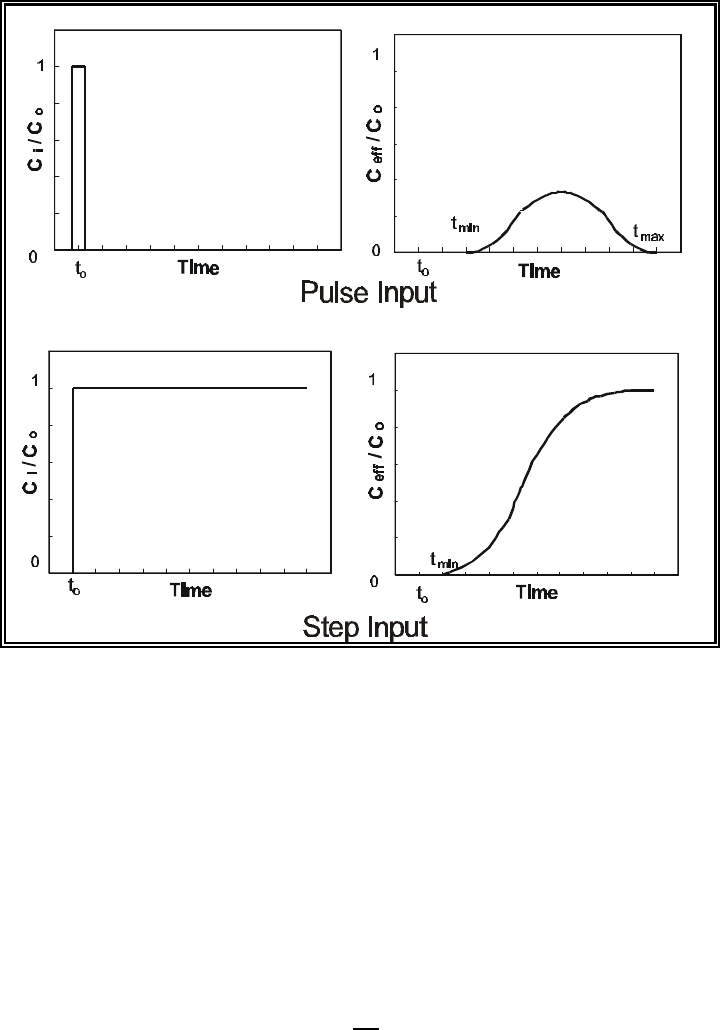
3.11

(3.7)

Figure 3.4. Schematic diagram showing the relative concentrations of a

constituent at the input source (figures on left) and in the

effluent (figures on right) as a function of time for a pulse

versus step input. [C

, C

, and C

eff

refer, respectively, to the

concentration of the constituent at t

and the concentrations

of the constituents in the input and effluent.]

The retardation factor (R

) is the ratio of the pore-water velocity (v

, cm/hr) to the contaminant

velocity (v

, cm/hr):

The pore-water velocity is operationally defined as the velocity of the nonadsorbing tracer.

3.12

(3.8)

' 1 %

(3.9)

' 1 %

(3.10)

' 1 %

(3.11)

The K

value can be calculated directly from the retardation factor (R

) and soil properties.

Depending upon the environmental conditions in which the contaminant moves and interacts with

the soil, the retardation factor can be correlated to the partition coefficient in a number of

different ways. At least 4 formulations of the retardation factor have been proposed [see reviews

in Bouwer (1991) and Whelan et al. (1987, 1996)]. These include the following:

where n = total porosity (cm

pore/cm

total volume),

= effective porosity (cm

pore/cm

total volume),

2 = volumetric water content in the vadose zone (cm

water/cm

total volume), and

= bulk density (g soil/cm

total volume).

Total porosity is the ratio of the air/water volume to the total soil. The effective porosity differs

from the total porosity in that the numerator is the volume of only those pore spaces that water

can travel through, excluding such void volumes as exist within aggregates or dead-end pore

spaces. Equation 3.10 was the original equation relating K

to R

. It was developed on an

empirical basis for use in chemical engineering and was first applied to groundwater situations by

Higgins (1959) and Baetslé (1967). Equations 3.8-3.11 were derived from the general transport

equation, which is the differential equation describing solute concentration changes in relation to

time, distance, dispersion coefficient, water velocity, soil bulk density, porosity, mass of solute per

unit dry mass of soil, and degradation of solute (Bouwer, 1991).

Equation 3.8 assumes that the soil has 2 types of pore spaces, those that permit flow to occur (n

and those pore spaces that do not permit flow to occur (n - n

). The contaminant in Equation 3.8

is assumed to migrate through the interconnected pore spaces, diffuse into dead-end pore spaces,

and instantaneously adsorb to or desorb from the soil matrix where fluid is and is not flowing.

Equation 3.8 also assumes that the solute concentration in the dead-end pore spaces is equivalent

to the solute concentration in the free-flowing spaces. Equation 3.8 has the appearance of being

more comprehensive than the other equations, but it does not allow the contaminant to travel with

the same speed as the fluid (i.e., nonadsorbing case), unless the total and effective porosities are

equal. Experience has shown that Equation 3.8 does not adequately reflect real-world

phenomena, suggesting deficiencies in our understanding of the geohydrochemical processes

3.13

impacting contaminant movement in the subsurface environment (Whelan et al., 1987).

Furthermore, in field studies, total porosity (n) can be measured directly, whereas effective

porosity (n

) can only be calculated from equations based on assumptions that are difficult to

defend (Freeze and Cherry, 1979).

Equation 3.9 includes the same processes as Equation 3.8, except that the contaminant does not

diffuse into the dead-end pore spaces. Many models use Equation 3.9 in their formulations. van

Genuchten and Wierenga (1986) suggest the use of Equation 3.10. Equation 3.10 includes the

same phenomena as Equation 3.9 except that the porous medium contains no dead-end pore

spaces. Again, the merit of its use over Equation 3.9 is that the measurable parameter n is

included in the formulation and not the calculated parameter n

. Equation 3.8, 3.9, and 3.10

describe chemical retardation in the saturated zone, whereas Equation 3.11 describes chemical

retardation in the unsaturated, or vadose, zone. As with Equation 3.10, contaminant transport

and retardation in Equation 3.11 occurs only in the free-flowing pore space. Bouwer (1991)

promotes the use of Equation 3.11 but defines the 2 term more generally as the water that is

moving, whether in unsaturated or saturated conditions. In his derivation of Equation 3.11,

Bouwer suggests that the 2 term also be used to quantify the mobile phases of water. Along with

van Genuchten and Wierenga (1986), he also contends that the use of Equation 3.11 allows better

distinction between retardation effects due to sorption and acceleration effects due to preferential

flow or anion exclusion.

Flow-through column experiments are appealing in that they allow observation of contaminant

migration rates in the presence of hydrodynamic effects (e.g., dispersion, colloidal transport, etc.),

and chemical phenomena (e.g., multiple species, reversibility, etc.). Ideally, flow-through column

experiments would be used exclusively for determining K

values, but equipment costs, time

constraints, experimental complexity, and data reduction uncertainties discourage widespread use.

One common problem in using column studies to measure K

values is that the breakthrough

curves are asymmetric. Such curves cannot be interpreted using Equations 3.8, 3.9, 3.10, or 3.11.

They require more complicated equations for solving for K

(Brusseau and Rao, 1989; van

Genuchten and Alves, 1982; van Genuchten and Wierenga, 1986).

One of the unique characteristics of measuring K

values from column experiments is that

nonequilibium conditions can be imposed. Especially under conditions in which the solute has

slow adsorption kinetics [e.g., those that may occur with uranium (Sposito, 1994)] or when

groundwater flow is fast, a measure of adsorption at equilibrium may over-estimate the extent to

which sorption occurs under actual field conditions. When either of these conditions are known

to exist in a study site, researchers should conduct column experiments at the flow rate existing in

the field, thereby creating realistic conditions.

Relyea (1982) provided an excellent review on the theoretical and experimental application of the

laboratory flow-through method of determining K

values. He reported that retardation factors

measured in column experiments depended on the water velocity and column dimension. For

short columns and slow water velocities, diffusion can become a major transport mechanism

3.14

(3.12)

resulting in lower retardation factors and lower K

values. At high velocities the effective pore

volume of a sample can decrease for short columns. High water velocities can also result in lower

retardation factors as a result of the solute not having sufficient time to adsorb to the soil, i.e.,

chemical equilibrium was not obtained. The effects of column length, mass of solute added to

column, diameter ratio of particle to column, and ratio of column diameter to column width on

the measured K

value were also presented by Relyea (1982).

3.2.4 Field Modeling Method

Field studies can provide accurate indications of the time of travel of the contaminant because the

concentrations of a dissolved contaminant are measured directly from samples taken from

monitoring wells. The field modeling method of estimating a K

value, also called the field

calibration method, uses a transport model and existing groundwater monitoring data. This

process, which is referred to as calibrating a groundwater transport model to K

values, involves

treating the K

value as an adjustable parameter (or dependent variable) while simulating

contaminant concentrations determined at monitoring wells. Groundwater calibration captures

the essence of the problem in the field. This is an iterative process that frequently requires the

adjusting the values for several other input parameters, such as effective porosity, dispersion, and

flow rate, to yield meaningful K

values. The minimum information that is needed for such a

calculation is the contaminant concentration at the source term, date of release, groundwater flow

path, groundwater flow rate, contaminant concentration at a monitoring well, distance between

source-release and monitoring well, dispersion coefficient, and source term. The retardation of

the chemical is then estimated as the ratio of the pore-water velocity to the contaminant velocity

(Equation 3.7). The pore-water velocity, v

, can be based on Darcy’s law (Freeze and Cherry,

1979) where

where v

= Darcy velocity

= effective porosity

However, 2 key drawbacks to this technique is that it is highly site specific and very model

dependent. Additionally, many assumptions have to be made about the water flow in the study

site including uniform flow and flow path. Not obvious, is that the K

value calculated by this

method greatly improves with more data. A detailed description of the theory of calculating K

values by this method and some examples of this approach are presented in Chapter 4.

3.2.5 K

Method

The extent to which an organic contaminant partitions between the solid and solution phases is

determined by several physical and chemical properties of the contaminant and soil (Lyman et al.,

1982). Since most sorption of hydrophobic organic substances is to the natural organic matter

present in sediments or soils, the usual approach is to assume that all sorption is to that matter and

Other limits have been suggested for the minimum organic fraction, f

, such as less than

0.1 percent (EPA, 1989) or less than a few tenths of a percent (Pignatello, 1989).

3.15

' K

(3.13)

to invoke a partition coefficient between organic carbon (K

) or organic matter (K

) and water

(Seth et al., 1999). Hydrophobic solutes appear to bind readily and rapidly with the outer surface

region in a few hours to a few days and then diffuse slowly into (and out of) the hydrophobic

interior region and narrow cavities in the sediment or soil organic matter during time periods of

weeks (Seth et al., 1999). An empirical approach that has had wide acceptance in the scientific

community is the organic-carbon partitioning coefficient (K

) method introduced by Karickoff et

al. (1979).

For this method, sorption of an organic contaminant, such as polynuclear aromatic hydrocarbon

(PAH), is assumed to occur only to the organic material in the soil. The partitioning between the

solid and solution phases is expressed as:

where K

= ratio of the contaminant concentration on the organic matter on a dry weight basis

to its dissolved concentration in the surrounding fluid (ml/g) and

= fraction of organic carbon in the soil (mg/mg).

Importantly, the K

method is only applicable for estimating organic compound partitioning.

Gschwend and Wu (1985) report that if precautions are taken to eliminate or account for

nonsettling microparticles or organic macromolecules which remain in the aqueous phase during

laboratory sorption tests, the observed organic-carbon partitioning coefficient have been found to

remain constant over a wide range of environmental and experimental conditions. However,

recent studies by Chiou et al. (1998) and Seth et al. (1999) indicate that for any given chemical,

an inherent variability in K

values is expected as a result of different environmental conditions

and equilibrium times. Dragun (1988) identified the following conditions when this approach is

less accurate:

C When the organic fraction, f

, is less than 1.0 percent

(LaGrega, 1994) or greater than

20 percent (EPA, 1988)

C When there are large amounts of swelling clays present (e.g., montmorillonite)

C When the partitioning organic compound is polar

C When mechanisms other than simple partitioning contribute to adsorption (e.g., cation-

exchange, anion-exchange)

C When a substantial time is required to reach equilibrium

The organic content of most soils falls in the range of 0.2 to 3.0% (LaGrega, 1994).

3.16

' "K

(3.14)

' 10

[57.735(C

) % 2.0(C

clay

) % 0.4(C

silt

) % 0.005(C

sand

)] .

(3.15)

The commonest correlation for K

is with the octanol-water partition coefficient (K

) for which

extensive databases and reliable estimation methods exist (Seth et al., 1999). A simplified

relationship between these two parameter is given by Equation 3.14.

where " = correlation coefficent (unitless).

LaGrega (1994) reports a value of (" = 0.63) as a commonly used value while Seth et al. (1999)

calculate a value of (" = 0.35) with a variation in " by a factor of 2.5 in either direction. Seth et

al. (1999) also suggested that K

estimates be viewed as a distribution, which includes

uncertainties about attainment of equilibrium and the variability in the composition of organic

matter present in soils and sediments, rather than as a single point value.

Strenge and Peterson (1989) applied the principle of the K

model to estimating the partition

coefficients for organic compounds on soils. They defined the K

for organic compounds through

the combination of the K

model and a parametric model (discussed in Section 3.4.2) based on

the concentrations of organic material (C

, percent w/w), clay (C

clay

, percent w/w), silt (C

silt

percent w/w) and sand (C

sand

, percent w/w) as dependent variables:

Equation 3.15 has the disadvantage of requiring more input parameters than Equations 3.13 and

3.14, but it provides an innovative approach for estimating the K

of organic compounds.

3.3 Issues Regarding Measuring and Selecting K

Values

3.3.1 Using Simple Versus Complex Systems to Measure K

Values

Soils are a complex mixture of solid, gaseous, and liquid phases. Each phase contains several

different constituents. Sposito (1989) estimated that the aqueous phase of a typical soil easily

contains between 100 and 200 different soluble complexes, many of them involving metal cations

and organic ligands (Table 3.1). The main effect of pH on these complexes, as is evident in

Table 3.1, is to favor free metal cations and protonated anions at low pH and carbonate or

hydroxyl complexes at high pH. The number of soluble complexes are also likely to be greater in

systems with elevated pH and organic matter concentrations. The solid phase in natural soils

typically contains more than 10 different constituents, including minerals, microbes, oxides,

naturally occurring organic matter, and organic, carbonate and/or oxide (e.g., iron, aluminum, and

manganese) coatings. The gas phase is quite different from that of above ground air as a result of

its interaction with the other phases and effects of pressure, temperatures, and microbial activity

(Sposito, 1989). For instance, the carbon dioxide levels is commonly several orders of magnitude

greater in soils than in above ground air (Wood and Petratis, 1984).

3.17

Table 3.1. Representative chemical species in acidic and basic soil solutions (after Sposito,

1989).

Cation

Principal Species

Acid Soils Alkaline Soils

Aluminum Al-org,

AlF

, AlOH

Al(OH)

, Al-org

Cadmium Cd

, CdSO

(aq), CdCl

, CdCl

, Cd SO

(aq), CdHCO

Calcium Ca

, CaSO

(aq), Ca-org Ca

, Ca SO

(aq), CaHCO

Chromium(III) CrOH

Cr(OH)

Chromium(VI) CrO

CrO

Copper(II) Cu-org, Cu

CuCO

(aq), Cu-org, CuB(OH)

Cu[B(OH)

]

(aq)

Iron(II) Fe

, FeSO

(aq), FeH

FeCO

(aq), Fe

, FeHCO

, FeSO

(aq)

Iron(III) FeOH

, Fe(OH)

(aq), Fe-org Fe(OH)

(aq), Fe-org

Lead Pb

, Pb-org, PbSO

(aq),

PbHCO

, PbHCO

, Pb-org, Pb(CO

)

PbOH

Magnesium Mg

, MgSO

(aq), Mg-org Mg

, MgSO

(aq), MgCO

(aq)

Manganese(II) Mn

, MnSO

(aq), Mn-org Mn

, MnSO

(aq), MnCO

(aq),

MnHCO

, MnB(OH)

Molybdenum(VI) H

MoO

(aq), HMoO

HMoO

, MoO

Nickel Ni

, NiSO

(aq), NiHCO

Ni-org

NiCO

(aq), NiHCO

, Ni

, NiB(OH)

Potassium K

, KSO

Silicon H

SiO

(aq) H

SiO

(aq)

Sodium Na

, NaHCO

(aq), NaSO

Zinc Zn

, ZnSO

(aq), Zn-org ZnHCO

, ZnCO

(aq), Zn-org, Zn

ZnSO

(aq), ZnB(OH)

Complexes for each cation are listed in the order of their relative concentrations from

greatest to lowest concentration.

Org / Organic complexes (e.g., fulvic acid complexes).

3.18

Scientists will conduct geochemical studies with pure phases, such as goethite, quartz, or

montmorillonite to work in well-defined systems. They may also choose not to work with actual

groundwater, but instead work with a “synthesized groundwater,” such as a calcium chloride

solution or a calcium chloride/sodium chloride solution. Again, the intent is to work in a

chemically well-defined system with as few constituents as possible. Experiments conducted

under simplified systems have provided information about the mechanisms by which solutes

interact with solid surfaces (Sposito, 1984; Sposito, 1989), information that otherwise would not

be possible to obtain from experiments conducted with natural heterogeneous soils and ground-

water.

Ideally, for site-specific calculations, the transport modeler should use sorption values determined

for site-specific materials at site-specific conditions. In the absence of such data, the modeler

often selects a K

value taken from the literature that was measured under similar conditions as

existing at the study site. However, as discussed in Chapter 2 (Section 2.2.3), very subtle

properties of the solid and aqueous phases can have a profound affect on a contaminants K

. For

example, only 1 percent (w/w) organic matter existing as surface coatings in a South Carolina

surface soil completely masked the surface properties of the underlying minerals (Kaplan et al.,

1993). The organic coatings imposed a much greater sorption potential than would have been

expected based on mineralogical considerations. Similarly, the surface properties of the soils just

below these soils were entirely dominated by iron-oxide coatings (Seaman et al., 1995). The

effect of the iron-oxide coatings was to create a solid phase that was dominated by pH dependent

charge surfaces. These subsurface soils adsorbed large amounts of anions because the pH was

below the zero-point-of-charge [discussed in Chapter 2 (Section 2.2.3)] of the iron oxides, pH ~8.

Subtle changes in the aqueous composition in a batch K

test may also have a profound affect on

the measured K

value (Delegard and Barney, 1983). Thus, it is essential for the modeler

selecting K

values to recognize which solid and aqueous phase components have a strong affect

on the sorption of the contaminant of interest. Identifying these important components is the

subject of Volume II.

3.3.2 Field Variability

The purpose of any soil sample is to obtain information about a particular soil. The sample itself

is seldom, if ever, the entire soil mass in which one is interested. In statistics, this larger aggregate

of material, in which we are ultimately interested, is called the “population.” Information from the

sample is of interest only insofar as it yields information about the population, and the information

may or may not be representative, depending on how the sample is selected.

The population itself may be large or small, or even a part of what the modeler considers a larger

population. For contaminant transport modeling, the population is commonly defined by either

stratigraphic units or soil texture. The justification supporting the use of these definitions is based

both on practical and scientific considerations. Soil texture and stratigraphy can be easily and

inexpensively determined from well-log data and the close correlation of a number of hydrological

and chemical properties with soil textures is well documented (Petersen et al., 1996). A some-

3.19

what better definition of soil populations would be the cation- or anion-exchange capacity of the

soils. However, this option is appreciably more expensive and is valuable only for defining K

populations. The soil texture data are also used for defining water flow populations.

The intensity with which a soil must be sampled to estimate with given accuracy some

characteristic, such as K

value, will depend on the magnitude of the variation within the soil

population under consideration. The more heterogeneous the population, the more intense must

be the sampling rate to attain a given precision. In general, although differences have been found

to exist among lithographic units, considerable variation may be expected within the units for such

characteristics as pH, phosphorous, potassium, sodium, conductivity, volume weight, permeability

and porosity (Peterson and Calvin, 1986). In some instances, the variation within contiguous

units is so great that it is not feasible to estimate differences between the units with any

satisfactory degree of precision. For most characteristics, the variation, both within and among

units, decreases, with increasing depth in the profile (Peterson and Calvin, 1986). Hence,

subsurface environments generally need to be sampled less than surface soils to attain comparable

accuracy (Mackay et al., 1986; Warrick and Nielsen, 1980). Mackay et al. (1986) reported that a

number of soil properties, including K

values, changed more vertically than laterally.

3.3.3 The “Gravel Issue”

Because most K

values are measured in laboratory studies, the sample size has an upper mass

limit of about 100 g soil (and often 10 g with the increased emphasis of waste minimization and

high disposal costs for laboratory wastes) in batch K

measurements and several kilograms of soil

in column studies. Both tests also have particle size limitations. The batch K

is typically limited

to the less than 2-mm size fraction (Appendix C, ASTM, 1987; EPA, 1991; Roy et al., 1991).

This size fraction was selected for a number of reasons that are both practical and scientific in

nature. The less than 2-mm fraction has historically been defined as the soil fraction and the

greater than 2-mm fraction as the rock fraction. The less than 2-mm fraction is also convenient

for most standard glassware used in batch K

tests (Figure 3.1). Another practical consideration

is that greater uniformity of the soil sample and therefore of the measured K

value can be

achieved if the range of particle sizes used in the test is limited. Finally, the smallest fraction is the

most chemically reactive fraction due to its high specific surface area (m

/g). The particle size

used in column studies is also commonly limited to the less than 2-mm fraction. This size fraction

was selected for similar reasons as for the batch studies and to compare results between the 2

common methods. However, Relyea (1982) indicated that the less than 2-mm size fraction should

only be used in columns greater than 80 mm in diameter. He indicates that to avoid local velocity

effects (e.g., channeling or a radial velocity gradient), the column diameter should be at least 30 to

40 times the particle diameter of the solids used to pack the column.

The “gravel issue” is the problem that transport modelers face when converting laboratory-

derived K

values based on experiments conducted with the less than 2-mm fraction into values

that can be used in systems containing particles greater than 2 mm in size. As mentioned above,

the less than 2-mm fraction is the more chemically reactive fraction due primarily to its large

3.20

µ g metal

g sediment

µg metal

ml solution

(3.16)

g metal

sediment

µg metal

ml solution

(3.17)

surface area. There are many subsurface soils dominated by cobbles, gravel, or boulders. To base

the K

values on the less than 2-mm size fraction, which may constitute less than 1 percent of the

soil volume, would grossly overestimate the actual K

of the aquifer. Including large soil particles

in a K

determination will increase the cost of laboratory equipment and perhaps more importantly

will result in K

values with large error terms because of the great variability of the particle size

distribution in subsamples of a single soil.

Two general approaches have been proposed to address the “gravel issue.” The first is to assume

that all particles greater than 2 mm have a K

= 0 ml/g. As an example, if 75 percent (w/w) of a

formation is composed of particles greater than 2 mm and the K

value of the less than 2-mm size

fraction was 100 ml/g, then the K

value used in the model would be 25 ml/g. Although the

assumption underlying this approach is incorrect, the extent to which sorption occurs on these

larger particles may be small. This approach is likely to yield a more accurate value in systems

dominated by cobbles, gravel, and boulders.

The second approach is to normalize laboratory-derived K

values by surface area. Thus, instead

of having units of

the laboratory K

value would have units of

(Kaplan et al., 1995b). Theoretically, this latter approach is more satisfying because it permits

some sorption to occur on the >2-mm fraction and the extent of the sorption is proportional to the

surface area. The underlying assumption in this approach is that the mineralogy is similar in the

less than 2- and greater than 2-mm fractions and that the sorption processes occurring in the

smaller fraction are similar to those that occur in the larger fraction. Because sorption is a surface

area phenomena (Equation 3.16), as opposed to a weight phenomena (Equation 3.17),

normalizing the data to surface area has logic, and is commonly done is soil (Sposito, 1989) and

colloid chemistry (Alberty, 1987). The drawback to this approach is that an additional

measurement is needed to calculate the newly defined K

value in the laboratory. Specific surface

area measurement is a rather common and simple procedure (Carter et al., 1986). This approach

3.21

to the “gravel issue” also requires a means to convert available soil texture data, which are often

available from well-hole logs or outcroppings of the formation, into surface area data.

3.3.4 The “Colloid Issue”

The “colloid issue,” as it pertains to measuring K

values, is the problem experimentalists have in

separating the aqueous from the solid phases during a laboratory batch K

measurement (see

Chapter 2). Typically centrifugation or filtration are used to accomplish this. If contaminants are

sorbed to tiny particles that remain in suspension after the separation step, the experimenter will

incorrectly assign the sorbed contaminant to the dissolved phase, C

(Equation 3.2). This will

result in underestimating the true K

value. This is an especially important problem for

contaminants that sorb strongly to solids, especially organic matter. Organic matter has a much

lower density than clay (i.e., ~1.05 g/cm

for organic matter versus ~2.6 g/cm

clays) and

therefore the common centrifugation protocol may not be sufficient to separate the phases. Also,

organic matter may exist as extremely small particles, or molecules, ~0.005 µm in diameter.

Thus, when a great deal of organic matter is present in a soil, or when only a trace amount of

organic matter has a profound affect on the measured K

, additional precautions must be followed

(Gschwend and Wu, 1985). For example, Gschwend and Wu (1985) reported that they were able

to increase the partitioning coefficient, which is related to the K

term (see Section 3.2.3), of

polychlorinated biphenyl by 3 orders of magnitude by very carefully removing unsettled organic

particles from suspension.

Using a centrifuge to make the solid and solution phase separations can also result in the

formation of a very thin zone at the liquid surface where surface tension holds fine-grained

particles at the top of the solution. The experimentalist should look for such problems and avoid

sampling the surface of the clarified liquid. When pipets are used to remove supernatant solution,

the pipet should be inserted sufficient distance below the surface to avoid drawing in suspended

particles, but to a distance where the pipet tip is above the settled solids-liquid interface to avoid

drawing in previously settled fines.

For these reasons, many experimentalists prefer to filter the supernatant solution after

centrifugation. Filtration does have its problems, however. Filtering a small volume of

supernatant solution can bias the contaminant’s concentration if the filter membrane adsorbs

solute species. The type of filter membrane used effects the potential for adsorption. In our

experience polyethylene or other plastic-based filter membranes are more inert than cellulosic-

based membranes. Filter membranes can also be “pre-treated” with the supernatant solution by

discarding the first aliquot and filtering a second aliquot that is saved for analysis. If the filter

membrane does adsorb the analyte of interest, the amount adsorbed usually rapidly diminishes as

the volume of solution filtered increases. Thus discarding the first aliquot of filtered solution and

using subsequent aliquots for analysis lowers the chances of biasing final K

values.

Another problem associated with colloids, is that the traditional 2-phase solute transport model

does not account for contaminants moving in association with mobile colloids. This subject is

3.22

discussed in Chapter 2 (Section 2.5.1). Briefly, contaminants with a high affinity for sorbing to

rock or vadose zone soils are assumed to be retarded relative to the rate of groundwater flow.

However, an increasing body of evidence indicates that under some subsurface conditions,

components of the solid phase may exist as colloids that may be transported with the flowing

water. Association of contaminants with this additional mobile phase may enhance not only the

amount of the contaminant that is transported, but also the rate of contaminant transport. Most

current approaches to predicting contaminant transport ignore this mechanism not because it is

obscure or the mathematical algorithms have not been developed (Corapcioglu and Kim, 1995;

Mills et al., 1991), but because little information is available on the occurrence, the mineralogical

properties, the physicochemical properties, or the conditions conducive to the generation of

mobile colloids. There have been numerous examples in which mobile colloids have been

implicated as the vector responsible for enhanced transport (Kaplan et al., 1994a,b; Kaplan et al.,

1995a; reviewed by McCarthy and Degueldre, 1993).

3.3.5 Particle Concentration Effect

Many investigators have observed that K

values determined in the laboratory often exhibit a

dependence with respect to the ratio of solid to solution used in the measurements. As recently

discussed by Oscarson and Hume (1998), this dependence is puzzling. From a theoretical

perspective, the K

value should not depend on the solid-to-solution ratio, because the definition

of the K

model (see Equation 2.20) normalizes the ratio of the solute sorbed to the solid to the

solute concentration left in solution based on the mass of solid and solution used for the

measurement. Thus the K

has units of volume/mass, such as typically ml/g.

Investigators have often found that K

values measured for many contaminants for a given soil-

groundwater system decrease as the solid-to-solution ratio increases. For example, this particle

concentration effect on K

values has been observed by O’Conner and Connolly (1980), Oscarson

and Hume (1998), Honeyman and Santschi (1988), Meier et al. (1987), and others. The same

trend with respect to particle concentration has also been observed for K

values for organic

contaminants [e.g., see Gschwend and Wu (1985) and Voice et al. (1983)].

Investigators have offered several explanations for the observed dependency. These explanations

can be categorized into two groups: (1) “real” physical/chemical processes, and (2) experimental

artifacts. One rationalization offered in the “real” category is that the particle concentration

effect is thought to be caused by particle-particle interactions. In systems with higher solids

content, these interactions are perhaps physically blocking some adsorption sites from the

adsorbing solutes and thus causing decreased adsorption, or creating electrostatic interferences

such that the electrical surface charges on the closely packed particles diminish attractions

between the adsorbing solutes and surfaces of individual grains. In terms of physical effects,

individual particles in a slurry having a high solid-to-solution ratio may have a greater tendency to

coagulate and flocculate into larger particles that have less available surface adsorption sites than

individual grains and thus can adsorb less adsorbate. This phenomenon is likely exacerbated by

diffusion processes that in short-term laboratory measurements, do not allow sufficient time for

3.23

the adsorbate to diffuse to the internal surface adsorption sites. The net effect is a K

measurement with a lower value when a high solid-to-solution ratio is present, because not

enough time was allocated for the water/soil system to reach a final equilibrium state. Thus there

are possible experimental artifacts even within the context of this “real” process explanation.

Plausible experimental artifacts also include less efficient separation of the solid phase from high

solids-content slurries, such that more colloidal size particles laden with adsorbate remain in the

solution phase and the associated adsorbate gets included in the analysis of the solution phase.

Complexing agents may desorb and/or dissolve from the solids, and in turn compete with the

adsorbate for the available sorption surface sites. Soluble organic carbon is a common example of

this process. Such effects increase when higher solid contents are used. Other artifacts include

changes in the aqueous system that are caused by mass transfer from the larger quantity of solids

but are not recorded during these measurements. Another consideration in the category of

possible experimental artifacts for the solid-to-solution effect is improper data reduction.

McKinley and Jenne (1991) suggest that the so-called particle concentration effect often goes

away when adsorption data are replotted as adsorption isotherms, where the mass of solute

adsorbed per mass of solid and the concentration of solute in the equilibrium solution are plotted

on the y- and x-axes, respectively.

The explanations for the particle concentration (solid-to-solution ratio) effect are numerous and

still rather perplexing [see summaries by Oscarson and Hume (1998) and Jenne (1998a)]. Jenne

(1998a,b) includes valuable discussion on this “solids concentration effect.” He also presents

some recommendations that should be followed when performing adsorption experiments and

identifies several key issues that should be addressed by future adsorption research. One practical

position that has been supported by EPRI (1991) is to conduct adsorption experiments as close as

possible to the conditions that exist at the site where contaminant mobility is being simulated and

assessed. In most cases, this recommendation would require that K

values determined by flow-

through column testing would be preferred over batch measurements conducted at low solid-to-

solution ratios.

As noted above, it has been suggested that K

values may decrease with increasing solid-to-

solution ratios. If this is a real effect, application of K

values based on a batch experiment

conducted with a solid-to-solution ratio significantly less than those that would exist in the field

would therefore overestimate the magnitude of contaminant sorption and underestimate the extent

of contaminant migration.

3.4 Methods of Acquiring K

Values from the Literature for Screening Calculations

3.4.1 K

Look-Up Table Approach: Issues Regarding Selection of K

Values

from the Literature

Clearly, the greatest limitation of using a K

value to calculate a retardation term (Equations 3.8,

3.9, 3.10, and 3.11) is that it describes solute partitioning between the aqueous and solid phases

3.24

for only 1 set of environmental conditions. K

values are known to vary greatly with only slight

changes in the composition of the solid and aqueous phases and these conditions often vary

greatly in 1 study site. For example, when the aqueous chemistry for a batch K

measurement

was varied, americium K

values in a Hanford sediment ranged from 0.2 to 53 ml/g, greater than a

200-fold difference (Delegard and Barney, 1983). Additional variability in the americium K

values were observed when slightly different Hanford sediments were used: 4.0 to 28.6 ml/g

(Delegard and Barney, 1983). Similarly, Sheppard et al. (1976) measured americium K

values

ranging from 125 to 43,500 ml/g using identical aqueous phases but different soils.

An alternative approach to a constant K

model is one in which the K

value varies as a function

of a select group of environmental conditions (Delegard and Barney, 1983; Routson and Serne,

1972; Strenge and Peterson, 1989). The easiest variable K

model to interface with a transport

code is one based on a look-up table. For look-up tables, separate K

values are assigned to a

matrix of discrete categories defined by chemically important environmental parameters (Strenge

and Peterson, 1989; Whelan et al., 1992). Strenge and Peterson (1989) used 9 categories defined

by soil pH and texture in the Multimedia Environmental Pollutant Assessment System (MEPAS)

code. The 3 soil texture classes were <10 percent, 10 to 30 percent, >30 percent clay/organic

matter/oxide content. The 3 pH classes were >9, 5 to 9, and <5. The 9 cells defined by the pH

and soil texture classes contained literature-derived K

values and where data was not available,

estimated values were included in the table. The inorganic contaminants in the K

look-up table

were actinium, aluminum, americium, antimony, arsenic, asbestos, barium, beryllium, borate,

cadmium, calcium hypochlorite, calcium oxide, carbon, cerium, chlorate, chromium (III),

chromium (VI), cobalt, copper, curium, europium, fluoride, hydrogen fluoride, iodine, iron,

krypton, lead, lead oxide, lithium hydroxide, lithium ion, magnesium, manganese, mercury,

molybdenum, neptunium, nickel, niobium, nitrate, nitric acid, nitrogen dioxide, palladium,

phosphate ion, phosphorus,, plutonium, polonium, potassium hydroxide, potassium ion,

protactinium, radium, ruthenium, samarium, selenium, silicate ion, silver, sodium ion, strontium,

sulfate, sulphur, thallium, thorium, tin, tritium, uranium, vanadium, yttrium, zinc compounds, zinc,

and zirconium.

For any literature-derived K

value, it is essential to clearly understand the selection criteria and

the logic used to estimate K

values not found in the literature. For instance, Strenge and

Peterson (1989) reported a wide range of literature K

values for several cells, typically greater

than 10-fold and sometimes greater than a 100-fold difference between minimum and maximum

values. The values included in the MEPAS look-up table were the minimum values found in the

literature. They justified this criteria because they wanted to build conservatism into the code.

Conservatism is traditional when addressing the extent of contaminant migration and associated

health effects, but may be erroneous if the modeling calculations are being used to address

remediation options, such as pump-and-treat remediation. Conservatism for remediation

calculations would tend to error on the side of under estimating the extent of contaminant

desorption that would occur in the aquifer once pump-and-treat of soil flushing treatments

commenced. Such an estimate would provide an upper limit to time, money, and work required

to extract a contaminant from a soil. This would be accomplished by selecting a K

from the

3.25

upper range of literature K

values. Thus, the K

values in MEPAS would not provide a conser-

vative estimate for clean-up efforts .

Other important issues regarding the use of literature-derived K

values are illustrated in

Table 3.2. In any K

look-up table, a small number of ancillary parameters must be selected to

define the cells. pH and soil texture were the ancillary parameters used in the MEPAS code.

These are excellent general categories for a large number of contaminants, however, they are of

only secondary importance to a large number of other contaminants. For example, the amount of

vermiculite, which is a 2:1 layer silicate mineral common in the United States, especially in the

west and mid-west, is arguable the single most important ancillary parameter affecting cesium

sorption (Douglas, 1989). Redox state is another example of an ancillary parameter that is

extremely important relative to affecting the removal from redox-sensitive contaminants solution

[this is actually a precipitation process and not an adsorption phenomena (Ames and Rai, 1978;

Rai and Zachara, 1984; Sposito, 1989)]. Some important redox sensitive contaminants include

arsenic, chromium, molybdenum, neptunium, plutonium, selenium, technetium, and uranium. The

values of uranium in the 9 MEPAS categories range from 0 to 500 ml/g (Table 3.2).

Table 3.2. Example of a K

(ml/g) look-up table for uranium, uranium(VI), and uranium(IV).

Material

$$ 9 5 - 9 ## 5

Fines

(%)

<10 10-30 >30 <10 10-30 >30 <10 10-30 >30

0 5 50 0 50 500 0 5 50

U(IV)

200 500 1,000 100 250 500 20 30 50

U(VI)

0 1 2 1 2 5 2 5 20

Fines (%) = sum of percentages of clay, organic matter, and hydrous-oxide in soil

Reference: Strenge and Peterson (1989)

Authors’ opinion based on values reported in Ames and Rai (1978), Ames and

McGarrah (1980), Cloninger et al. (1980), Cloninger and Cole (1981), Serne and Relyea

(1981), and Rai and Zachara. (1984).

By including an additional ancillary parameter of oxidation state, appreciably greater accuracy can

be assigned to K

values. For U(VI), the 9 categories may be assigned K

values in the range of 0

to 20 ml/g, whereas, as for U(IV), the 9 categories may be assigned K

values in the range of 20

to 1,000 ml/g. In this example, oxidation state is obviously a more important ancillary parameter

than soil texture and in systems with pH values greater than 5, oxidation state is more important

Strenge and Peterson (1989) generated most of the values in the pH>9 categories by

multiplying the K

values from the pH 5 to 9 category by 0.1. A significant quantity of K

values

exist in the literature for the latter pH category. The “0.1 factor” was based on consistent, but

flawed logic that metal contaminants are less likely to sorb because their cationic valence

decreases by [M

(OH

)]

a-x

. It is now known that hydrolysis species adsorb as well as or better

than free cations (M

). Also many contaminants precipitate at higher pH values, giving the

appearance of increased K

values. There are a few exceptions in pH >9 systems: Zr(OH)

species that may not adsorb as well as Zr

, and UO

(CO

)

and UO

(CO

)

species do not

adsorb as well as the UO

and UO

species. The CO

activity increases as pH increases so

complexes get more important at elevated pH levels.

3.26

than pH. The reduced form of U, U(IV), has a much greater K

value than U(VI) because the

former is known to precipitate from solution. The rather low uranium K

values reported by

Strenge and Peterson (1989) are somewhat misleading in that they represent, as mentioned above,

minimum values identified in the literature. These values would be entirely inappropriate for

modeling U(IV) transport. Thus, an important point to this discussion is that no single set of

ancillary parameters, such as pH and soil texture, is universally appropriate for defining categories

in K

look-up tables for all contaminants. Instead, the ancillary parameters used in look-up tables

must be based on the unique chemical properties of each contaminant.

An apparent inconsistency in Table 3.2 is that the minimum values selected by Strenge and

Peterson (1989) for the uranium data are greater than those for U(VI). This inconsistency is not

due to differences in literature used to estimate these values. Instead it arises from differences in

how K

values are estimated for cells in which no data are available.

This illustrates another

important reason for clearly understanding the criteria and process used in selecting data

incorporated into a look-up table. Clearly, differences in the criteria and process used to select K

values can result in appreciable different values included in a look-up table; in this example, as

much as 3 orders of magnitude.

3.4.2 Parametric K

Approach

The parametric K

approach is similar to that of the K

look-up table approach in that it varies K

values used in a transport model as a function of important ancillary parameters. It differs from

the K

look-up table in that it uses a regression equation to define the K

values instead of using

discrete categories. The K

value in this model varies as a function of empirically derived

relationships with aqueous and solid phase independent parameters. Thus, it has the distinct

advantage over look-up tables of having a continuum of K

values.

Factorial design experiments are most often used to determine the systematic change resulting

from varying the independent variables (e.g., pH, soil texture, and redox status) on the dependent

variables (uranium K

) (Box and Behnken, 1960; Cochran and Cox, 1957; Davies, 1954; Plackett

and Burman 1946). Statistical methods commonly used to derive quantitative predictor equations

include standard linear or nonlinear regression (Snedecor and Cochran, 1967), stepwise regression

3.27

Log K

(Americium) ' 2.0 % 0.1[NaOH] & 26.8[HEDTA] % 153.4[HEDTA]

(3.18)

(Hollander and Wolfe, 1973), and adaptive-learning networks (Mucciardi et al., 1979, 1980). All

these techniques have been used to develop empirical relationships describing K

values in terms

of other variables (Delegard and Barney, 1983; Routson and Serne, 1972; Serne et al., 1973;

Routson et al., 1981).

The empirical predictor equations commonly take the form of a nonlinear polynomial expression.

For example, after evaluating solutions consisting of several sodium salts, organic chelates, and

acids, Delegard and Barney (1983) came up with the following expression for an americium K

value:

where HEDTA is N-(2-hydroxyethyl) ethylenediaminetetraacetic acid. Numerous salts were

found to have no significant effect on americium K

values and therefore were not included in the

expression. Delegard and Barney (1983) also evaluated higher exponential and logarithmic terms

and determined that these terms did not improve the predictive capabilities of the expression (i.e.,

the regression coefficients were not significant at P # 0.05).

It is critical that parametric K

equations, such as Equation 3.18, be used to calculate K

values

for systems within the range of the independent variables used to create the equation. In the case

of Equation 3.18, the range of independent variables used in generate the model were selected to

simulate a plume beneath the Hanford Site in Richland, Washington. Using Equation 3.18 to

generate americium K

values for a plume low in pH and Na concentrations would not be

appropriate.

These types of statistical relationships are devoid of causality and therefore provide no certain

information regarding the mechanism by which the contaminant partitioned to the solid phase,

whether it be by adsorption, absorption, or precipitation. For example, the statistical analyses

may suggest a very strong relationship between pH and the K

term, when the actual sorption

process may be controlled by iron oxide adsorption. Because pH and iron-oxide charge are

covarients, a statistical relationship may suggest that sorption is due to pH, when in fact,

suggesting that sorption is solely caused by pH.

The parametric K

model is used in the transport equation, the code must also keep track of the

current value of the independent variables (e.g., [NaOH] and [HEDTA] for the examples

described in Equation 3.18) at each point in space and time to continually update the

concentration of the independent variables affecting the K

value. Thus, the code must track

many more parameters, and some numerical solving techniques (e.g., closed-form analytical

solutions) can no longer be used to perform the integration necessary to solve for concentration.

Generally, computer codes that can accommodate the parametric K

model use a chemical

subroutine to update the K

value used to determine the R

, when called by the main transport

code. The added complexity in solving the transport equation with the parametric K

sorption

model and its empirical nature may be the reasons this approach has been used sparingly.

3.28

3.4.3 Mechanistic Adsorption Models

Mechanistic models explicitly accommodate for the dependency of K

values on contaminant con-

centration, competing ion concentration, variable surface charge on the adsorbent, and solute

species solution distribution. Incorporating mechanistic, or semi-mechanistic, concepts into

models is attempted because the models become more robust and, perhaps more importantly from

the standpoint of regulators and the public, scientifically defensible. The complexity of installing

these mechanistic adsorption models into existing transport codes is difficult to accomplish.

Additionally, these models also require a more intense and costly data collection effort than will

likely be available to the majority of contaminant transport modelers who are conducting

screening calculations. Descriptions of the state of this science, with references to excellent

review articles, are presented in Chapter 2 and 5. A review of the methodology associated with

the determination of the constants for use in these mechanistic models, however, is beyond the

scope of this project. A review of the mechanistic adsorption models contained in EPA’s

MINTEQA2 geochemical reaction code is also presented in Chapter 5.

3.5 Summary

The objective of this chapter is to describe methods used to measure K

values. The advantages

and disadvantages and the assumptions underlying each method were discussed, and are

summarized in Table 3.3. A number of issues regarding the selection of K

values from the

literature for screening calculations are also addressed in this chapter. Specific issues discussed

included the use of simple versus complex systems to measure K

values, field variability, the

“gravel issue,” and the “colloid issue.”

Clearly, the greatest limitation of using a K

value to calculate a retardation term is that it is only

applicable to a single set of environmental conditions. Consequently, researchers have generated

values that varies as a function of ancillary environmental parameters. They include the look-

up table K

, the parametric K

, and the mechanistic K

. Models generated for parametric K

values have typically been for rather limited environmental conditions. Mechanistic K

values are

limited to uniform solid and aqueous systems with little application to the heterogenous soils that

exist in the natural environment. The easiest and the most common variable K

model to interface

with a transport code is the look-up table. No single set of ancillary parameters, such as pH and

soil texture, is universally appropriate for defining categories in K

look-up tables. Instead, the

ancillary parameters must vary in accordance to the geochemistry of the contaminant. It is

essential that the modeler fully understand the criteria and process used for selecting the values

incorporated in such a table. Just as important is to understand the logic used to estimate K

values not found in the literature. Differences in the criteria and process used to select K

values

can result in appreciable different K

values.

It is incumbent upon the transport modeler to understand the strengths and weaknesses of the

different K

methods and perhaps more importantly the underlying assumption of the methods in

order to properly select K

values from the literature. The K

values reported in the literature for

3.29

any given contaminant may vary by as much as 6 orders of magnitude. An understanding of the

important geochemical processes and knowledge of the important ancillary parameters affecting

the sorption chemistry of the contaminant of interest is necessary for selecting appropriate K

value(s) for contaminant transport modeling.

3.30

Table 3.3. Advantages, disadvantages, and assumptions of different methods used to determine

and the assumptions in applying these K

values to contaminant transport models.

Methods for Determining K

Batch

In-Situ Field Batch

Flow-Through Field Modeling K

Minimum Input Data

C M

sed

C C

C V

C C

C A

(or q

)

C C

C n, 2, or n

C D

particle

C >10 C

effluent

data

points

C C

tracer

C Time

C C

release

C C

well

C Time

C Distance

C v

C n, 2, or n

C Diffusion or

dispersion

coefficients

C K

C f

Advantages

C Inexpensive

C Quick

C In-situ

measurements

C Equilibrium

conditions

C Aqueous and solid

phases are precisely

those of the

modeled system

C Can measure sorp-

tion at field flow

rates, i.e., at non-

steady state condi-

tions

C Can measure hydro-

dynamic effects

(e.g., dispersion,

colloidal transport,

etc.) on R

, and

subsequently incor-

porate into

value

C Can measure effects

of chemical

phenomena (e.g.,

multiple species,

reversibility, etc.) on

and K

values.

C Derived K

has the

precise geochemical

conditions and flow

conditions of the

study site

C Fairly accurate

indirect method

C Often can use look-

up tables to get K

value

C f

is an easy

measurement

C K

can be

correlated with K

which has been

measured for many

different chemicals

3.31

Table 3.3. Continued.

Methods for Determining K

Batch

In-Situ Field Batch

Flow-Through Field Modeling K

Disadvantages

C Provides estimate of

chemical processes

at equilibrium; flow

conditions are not

always at

equilibrium

C Physics involved not

considered

C Better mixing in

batch than in nature

C Typically uses larger

ratio of solution/soil

than exist in nature

C Experiments

measure adsorption

instead of

desorption, the

dominant process in

transport; desorption

is typically much

slower than

adsorption

C Speciation of

different forms not

considered

C Expensive to collect

samples

C Commonly have

high detection limits

(undesirable) for

measuring

contaminant on

solid phase (A

, q

)

C Site-specific data

C Cannot

unequivocally

differentiate

between, adsorbed,

precipitated, and

structural

constituents

C Commonly flow-

through system is

not at equilibrium

and therefore results

cannot be applied to

other flow

conditions

C Directly measure R

then back out K

;

therefore must make

assumptions about

relation between K

and R

C Measured K

values

commonly vary with

water velocity and

column dimensions

C Requires relatively

expensive

equipment

C Requires a lot of

time

C Complex experiment

to conduct

C Data are commonly

not well behaved,

i.e., asymmetric or

peakless break-

through curves

C Can investigate

some secondary

processes affecting

contaminant

transport, such as

effects of

unsaturated flow,

colloid-facilitated

contaminant

transport, mobile vs

immobile water

phases

C K

is truly site

specific

C K

is transport model

specific

C Need to make many

assumptions about

the water flow

including uniform

flow, direction, and

path length that

affect the calculated

value

C Measure R

, then

back out K

; many

assumptions go into

relating K

to R

C May or may not be in

equilibrium,

therefore not a

thermodynamic K

C K

value greatly

improves with more

field data collected

C Calculations can be

quite involved

C For organic

compounds only

C More hydrophobic

the contaminant

compound, more

accurate the K

; vice

versa with

hydrophilic

compounds

3.32

Table 3.3. Continued.

Methods for Determining K

Batch

In-Situ Field Batch

Flow-Through Field Modeling K

Assumptions in Calculating K

C Adsorption rate =

desorption rate

C Only 1 type of

surface adsorption

site, A

C Only 1 type of

aqueous dissolved

species, C

C A>>>A

C Activity of A

C Equilibrium has

been achieved

during mixing

period

C No adsorbate on

suspended colloids

C No precipitation of

adsorbate due to C

concentration

exceeding solubility

C Same as for batch

C Measurement of

adsorbed

contaminant, A

can differentiate

between adsorbed,

precipitated, and

structural

constituents

C Must assume a

relationship between

and K

C Water flow and

dispersion

coefficient is

constant

C Must assume a

relationship between

and K

C Know n

or n

C Must know the flow

path and velocity of

plume

C Sorption is uniform

in the study size

C Same as for

laboratory batch K

C Organic

contaminant sorbs

(partition) only to

organic matter in

soil, no sorption

occurs to inorganic

phases

3.33

Table 3.3. Continued.

Methods for Determining K

Batch

In-Situ Field Batch

Flow-Through Field Modeling K

Assumptions in Applying Measured K

to Transport Model

C Adsorption of solute

is linear, i.e., it is

independent of C

C Adsorption of solute

is reversible

C Solute movement is

slow enough that

equilibrium

conditions exist

between the solute

and soil

C Geochemical

conditions (presence

and concentration of

background

electrolytes and

solid phases) of

batch experiment are

identical to those in

aquifer

C Temperature and

pressure conditions

of batch experiment

are identical to those

in the aquifer

C Mixing in aquifer is

as thorough as in

batch experiment

C Difference between

the soil/water ratio

in the aquifer and

batch experiment is

not important to K

value

C Same as for

laboratory batch K

(except fourth point

not relevant to

in-situ batch

method)

C It is more common

to enter the R

value

derived from

experiment than the

value into

transport code;

consequently, do not

need to make any

assumptions about

the relationship

between R

and K

C If R

value from

column experiment

is entered into

transport code and

the flow conditions

of the experiment

are similar to those

in the site being

modeled, then no

assumptions need to

be made regarding

affect of

nonequilibium

conditions

C None C Same as for

laboratory batch K

See Equation 3.4

See Equation 3.13

A = Concentration of free or unoccupied surface adsorption site on a solid phase; C

= the total dissolved adsorbate

concentration remaining in solution at equilibrium; f

= fraction of soil that is organic carbon; C

release

= concentration of

solute at time of release; C

well

= concentration of solute in monitoring well; M

= soil mass; A

= the concentration of

adsorbate on the solid at equilibrium; n = total porosity; n

= effective porosity; V

= solution volume; D

= bulk density;

particle

= particle density; 2 = water saturation.

particle

is used to calculate bulk density (D

); D

= [D

particle

(1 - n)].

See Equations 3.8, 3.9, 3.10, and 3.11.

A list of acronyms, abbreviations, symbols, and notation is given in Appendix A. A list of

definitions is given in Appendix B

4.1

4.0 Groundwater Calibration Assessment Based on Partition

Coefficients: Derivation and Examples

4.1 Introduction

Partition (or distribution) coefficient, K

values are utilized in transport and risk assessment

modeling because of their simplicity in (1) understanding, (2) measuring, and (3) providing

closed-form, explicit, analytical solutions to the advective-dispersive equations. Whelan (1996)

presented a discussion that illustrates the inherent difficulties associated with utilizing partition

coefficients as the sole parameter to define the geochemical properties of a solute as it migrates

through a subsurface environment. Multiple definitions for K

values have been identified,

including those based on thermodynamics (e.g., Gibbs free energy of formation), experiments

(e.g., batch and flow-through tests), and theory (e.g., isotherms). Each of these procedures

identifies a different value for the same parameter, which is supposed to describe the same

phenomena. Although K

values can be thermodynamically defined, their meaning becomes less

clear in the real world. As such, K

values can be estimated using transport models. This process,

called calibrating a groundwater transport model to K

values, involves treating the K

value as

the adjustable parameter (or dependent variable) while simulating known monitored contaminant

data. Groundwater calibration captures the essence of the problem in the field. This is an

iterative process that frequently requires that the magnitude of a number of other input

parameters, such as effective porosity, dispersion, and flow rate, be adjusted to yield meaningful

values. A K

value represents one of the calibration parameters because its magnitude is

subject to not only the laboratory analyses but also to the heterogeneity in the field and different

ways it is used in the mathematical constructs of different models.

4.2 Calibration: Location, Arrival Time, and Concentration

When calibrating a groundwater model to monitored information (e.g., concentrations at a

monitoring well), the model must predict the correct arrival time at the correct location, matching

the magnitude of the monitored concentration. Therefore, time, location and magnitude are

3 crucial elements associated with any calibration exercise, and K

impacts two of them (i.e.,

travel time and magnitude). Location is predetermined by the user with respect to monitoring

wells, receptor locations, etc. Once the distances have been defined, the calibration requires

modifications to parameters that govern travel times and concentration levels. Parameters, which

influence water and contaminant movement, are varied within acceptable ranges in an attempt to

recreate conditions in the field. As the model complexity increases, the number of parameters that

the analyst can vary increases, and the calibration process becomes increasingly more

complicated. Figure 4.1 illustrates the relative relationships between input-data quality, output

uncertainty, and types of problems addressed by each level of assessment. As Figure 4.1 indi-

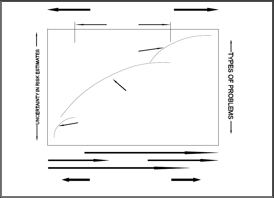
4.2

LEVEL OF ANALYSIS

specific

site-

broad

range

least

greatest

screening

analytical

numerical

analytical

screening

numerical

INPUT DATA QUALITY

site-specific

regional

representative

highestleast

cates, the computational requirements tend to be less at the earlier stages of an assessment when

available data are less, and, correspondingly, the uncertainty with the output results tends to be

greater. As the assessment progresses, improved site-characterization data and conceptualization

of the problem increase, thereby reducing the overall uncertainty in risk estimates.

Figure 4.1 also illustrates some of the characteristics and relationships between screening-level

(ranking), “analytical” (prioritization and preliminary assessments), and numerical (detailed)

models.

Figure 4.1. Relative relationships between input-data quality, output uncertainty, and types

of problems addressed by each level of assessment.

4.3

Screening models are used to identify environmental concerns. These models, often based on a

structured-value approach, are designed to be used with regional/representative information.

Models such as the Hazard Ranking System (HRS) (EPA, 1984, 1992b) divide site and release

characteristics into predetermined categories that are assigned a point value based on answers to

questions. The score from such systems is useful to determine if a situation requires further

analysis, but not to provide a method for estimating actual concentrations or impacts in the

environment.

Detailed analyzes require a highly specialized assessment of potential impacts. Detailed analyses

are usually reserved for the most complex models, are data intensive, and are based on the

expertise of the analyst. These detailed assessment models are used to address complex problems

and concerns that are relatively well-defined. Models for detailed analyses tend to focus on

special sets of problems and special types of situations. Although detailed assessment tools are

appropriate for their intended application, extension beyond the site-specific application is often

difficult or cost prohibitive. Typical models include MODFLOW (McDonald and Harbaugh,

1988) and CFEST (Cole et al., 1988).

Analytically/semianalytically/empirically based models (designated as “analytical” models in

Figure 4.1) can be utilized for prioritization or preliminary assessments and exist between initial-

screening and highly specialized numerical models. These physics-based models are the most

versatile as they do not have the data constraints associated with the numerical models. The

analytical models may contain some numerical computations, hence the semianalytical designa-

tion. As Figure 4.1 illustrates, the analytical models are designed to provide environmental

evaluations over a wide range of applications. Groundwater models that fall into this category

include AT123D (Yeh, 1981), GROUND and GRDFLX (Codell et al., 1982), and MEPAS (Buck

et al., 1995; Whelan et al., 1992). The analytical-assessment models are codes with physics-

based algorithms whose components can be utilized in a detailed (i.e., numerical) or an initial-

screening (i.e., ranking/prioritization) assessment, where data and circumstances warrant.

The calibration process is an interactive one. Because data tend to be limiting, there are generally

multiple ways in which parameters can be combined so the simulation results match monitored

information. With increasing number of monitored data available, less combinations of the

modeling parameters are possible to match the monitored information. In addition, many of these

“matches” can assign unrealistic values to parameters; therefore, the number of acceptable

possible combinations becomes even more limited. When calibrating, parameters can only be

varied within ranges that physically make sense for the site and its conditions. If unrealistic

output is a result of the analysis, then the (1) conceptual site model has to be re-evaluated, (2)

input data must be re-examined, and/or (3) model must be re-evaluated to ensure that the

assessment does not violate the assumptions, limitations, and constraints associated with the

mathematical constructs of the code.

Each code has its own mathematical equations upon which it is based. A calibration exercise is

performed to meet the constructs of these equations. Analytical models tend to be easier to work

4.4

% v

(

M C

' D

(

% D

(

% D

(

M z

& 8 C

(4.1)

with because of their closed-form, explicit solutions. With an analytical model, some initial

calculations can be made that can provide an initial starting point for the calibration process; this

process also illustrates how retardation factors (and ultimately K

) influence the calibration

process. As noted earlier, the intent of the calibration process is to get a contaminant from a

source to the monitored location (e.g., monitoring well) at the proper time with the appropriate

concentration. In addition, the amount of mass monitored in the environment must be conserved,

that is, the amount of mass predicted by the model to be in the environment should match the

amount of mass monitored in the environment.

Travel times are influenced by the retardation factor, pore-water velocity, and dispersivity,

although other parameters can also influence the outcomes. The retardation factor can be directly

impacted by K

. In the vadose zone, soil type and moisture content influence pore-water velocity,

and in the saturated zone, soil type and effective porosity influence pore-water velocity.

Longitudinal dispersivity normally influences the time to peak but by no more than 10 percent,

although more is possible. Concentrations are generally influenced by the contaminant flux rate

(or total mass released into the environment), mixing distances (dilution), pore-water velocity

(dilution), retardation factor (K

), and dispersivity (dispersion). If the size of the source is not

well known, the areal extent of contamination influences concentration levels for spatially near-

field problems. In any modeling exercise, the analyst will know some of the general charac-

teristics of the parameters. Typically, the parameters that are used to calibrate the model are not

known exactly; therefore, they can be modified within an appropriate range to help the analyst

capture the essence of the problem.

4.3 Illustrative Calculations to Help Quantify K

Using Analytical Models

If K

forms the basic premise for retarding the movement of contaminants in a subsurface

environment in the mathematical algorithms of a groundwater transport code, then the K

permeates all of the contaminant transport calculations. Different computer codes may use

different mathematical constructs, but the influence of K

is usually very pronounced. The K

value influences the calculations for determining the (1) contaminant travel time, (2) mass of

contamination at the source or in a plume, and (3) distribution of the concentration in the

environment. As an illustration of the impact that the K

parameter can have in transport

calculations, the influences of K

on an analytical solution to the advective-dispersive equation are

explored.

4.3.1 Governing Equations

The 1-dimensional advective, 3-dimensional dispersive equation with first-order

degradation/decay can be expressed as follows:

4.5

(

(4.2)

(4.3)

' 1 %

saturated

(4.4)

' 1 %

vadose

(4.5)

(4.6)

(

mech

% D

mol

(4.7)

mech

' " v

(4.8)

in which

where C

= dissolved concentration

v* = contaminant velocity

D* = dispersion coefficient in the x, y, and z directions adjusted for retardation with

the retardation factor

8 = first-order degradation/decay coefficient

= pore-water velocity

= Darcy velocity

= retardation factor

= effective porosity

= bulk density

= moisture content in the vadose zone

= partition (distribution) coefficient

= adsorbed contaminant concentration on the soil particles

mech

= mechanical dispersion

mol

= molecular diffusion coefficient

4.6

' *' X

(4.9)

*' '

rel

(4.10)

4 B D

(

1/2

exp (&8 t) exp &

(x & v

(

4 D

(

(4.11)

4 B D

(

1/2

exp &

4 D

(

(4.12)

(4.13)

" = dispersivity in the x, y, or z direction

The solution of advective-dispersive equation for an instantaneous release through a point source

in a saturated zone, which is uniformly mixed in the vertical direction, at a distance (x) down

gradient from the center of the source is as follows (Codell et al., 1982; Fischer et al., 1979;

Whelan et al., 1996; Yeh and Tsai, 1976; Yeh 1981):

where *' = mass-related constant

, Y

, and Z

= Green's functions (which are orthogonal) in the x, y, and z

directions, respectively

= Green’s function corresponding to flow direction

in which

where M

rel

= released mass

y = off-centerline distance

= mixing-zone thickness

and all other parameters retain their previous definitions.

The impact that the retardation factor and, hence, K

has on the calculated value of the

concentration at the receptor location can be profound, as illustrated by the number of locations

that these terms appear in the governing equations.

4.7

(

(4.14)

' t

% t

(4.15)

) 1 %

(4.16)

> '

(4.17)

1 %

(4.18)

4.3.2 Travel Time and the Partition Coefficient

As previously noted, it is very important to ensure that the contaminant arrives at the monitoring

location at the appropriate time, and K

can have a profound impact on the travel time. The

advective travel time of the contaminant is defined as the distance x traveled divided by the

contaminant velocity:

where t

= total advective travel time of the contaminant

If a contaminant is traveling from a contaminated source through a vadose zone, through a

saturated zone to a monitoring location, the total advective travel time is the summation of the

travel times through the vadose (t

) and saturated (v

sat

) zones:

where H

= thickness of the vadose zone

subscripts 1 and 2 = vadose and saturated zones, respectively

Substituting the definitions for retardation factor gives a slightly modified equation:

This equation demonstrates the potential impact that K

has on the travel time. Because K

assumed to be constant over the distanced traveled, a constant, >, can be defined, which

represents the ratio of the partition coefficients between the vadose and saturated zones:

Substituting > into the total travel time equation gives the travel time as a function of the saturated

zone’s partition coefficient:

4.8

(4.19)

& (H

) & (x

)

(4.20)

(4.21)

ads

' V

source

1 & n D

particle

(4.22)

source

(4.23)

Rearranging this equation and solving for K

gives:

This equation can be used to estimate initial values for the partition coefficients in the vadose and

saturated zones, which will help ensure that the contaminant reaches the monitoring location at

the appropriate time. These values can also be compared to literature or experimental values to

see if they are consistent. If not, then the conceptual site model must be re-analyzed to ensure

that the proper problem has been captured or that the appropriate data are being utilized.

4.3.3 Mass and the Partition Coefficient

The partition coefficient can be used to help estimate the mass of contamination that exists at the

source or in a plume. The reported soil contamination in the vadose zone is usually expressed as

the adsorbed concentration (A

) and typically has units of mg/kg, which is also expressed as ppm

(parts per 10

). The aqueous concentration (C

), using K

as a conversion factor, can be

calculated as follows:

The mass associated with the adsorbed phase in the vadose zone can be estimated as:

where M

ads

= mass associated with the adsorbed phase in the vadose zone

source

= volume associated with the contaminated source

n = total porosity

particle

= particle density

The mass associated with the aqueous phase in the vadose zone can be estimated as:

4.9

vadose

' M

ads

% M

vadose

(4.24)

' V

source

(4.25)

ads

' V

source

1 & n D

particle

(4.26)

saturated

' M

ads

% M

saturated

(4.27)

Total

' M

vadose

% M

saturated

(4.28)

% D

(4.29)

% D

(4.30)

where M

= mass associated with the aqueous phase in the vadose zone

The total mass associated with the vadose zone represents the summation of the mass associated

with the adsorbed and aqueous phases, assuming no free product:

where M

vadose

= total mass associated with the vadose zone

The reported aqueous contamination in the saturated zone is usually expressed as the dissolved

concentration C

and typically has units of mg/l, which is also expressed as ppm (parts per 10

The mass associated with the aqueous phase in the saturated zone can be estimated as:

The mass associated with the adsorbed phase in the saturated zone can be estimated as:

The total mass in the vadose zone represents the summation of the mass associated with the

adsorbed and aqueous phases, assuming no free product:

where M

saturated

= total mass associated with the saturated zone

The total mass in the system is the summation of the masses in the vadose and saturated zones:

If the environmental contamination in the vadose zone is expressed as a total mass in the waste

site (or layer) per dry weight of soil, the dissolved and adsorbed concentrations can be calculated

as follows (Whelan et al., 1987):

where C

= total mass at the site per dry weight of soil

4.10

% D

(4.31)

% D

(4.32)

' D

(

(4.33)

(2 B)

1/2

exp &

2 F

(4.34)

' 2 D

(

1/2

2 D

1/2

(4.35)

' "

(4.36)

If the environmental contamination is expressed as a total mass per total volume of the waste site

(or soil layer), the dissolved and adsorbed concentrations can be calculated as follows (Whelan et

al., 1987):

where C

= total mass at the site per total site volume

4.3.4 Dispersion and the Partition Coefficient

The 1-dimensional, dispersive equation in the lateral direction can be expressed as

where all of the terms are as previously defined. For an instantaneous release from a unit area in

an aquifer of infinite lateral extent, the time-varying concentration as a function of lateral distance

off the center line can be expressed as follows:

in which

where M

= instantaneous mass released per unit area (i.e., instantaneous point-source release)

= standard deviation associated with the Gaussian solution

Note that the standard deviation (i.e., the degree of lateral spreading) is a function of the

retardation factor and, hence, K

4.11

t '

x R

(4.37)

' 2 "

1/2

(4.38)

To gain an understanding of the impact of the retardation factor (and K

) on simple advective-

dispersive systems, the impact of retardation at a location, x, can be discerned by substituting the

time, t, with the advective travel time, as follows:

The standard deviation that indicates the degree of spread at location x is independent of the

retardation factor and K

. This phenomenon is expected because when combined with flow in the

longitudinal direction, advection impacts the effects of dispersion in the lateral direction. In

effect, advection transports the contaminant in the longitudinal direction, so there is no infinite

dispersion at any location in the lateral direction. Hence, Gaussian plumes grow as they migrate

down gradient. Unlike the contaminant travel time, the dispersive phenomenon is not closely tied

to K

4.4 Modeling Sensitivities to Variations in the Partition Coefficient

Because the retardation factor and partition coefficient permeate many aspects associated with the

mathematical algorithms for contaminant transport in the subsurface environment, K

can have a

significant impact on the outcome of any modeling exercise. Under certain circumstances though,

can have very little impact on the outcome. The next 2 sections discuss the conditions under

which partition coefficients influence the outcome.

1. Relationship Between Partition Coefficients and Risk -- This section explores the

situations under which variations in K

can have a significant influence on simulated

groundwater concentrations and, hence, risk.

2. Partition Coefficient as a Calibration Parameter in Transport Modeling -- This section

presents an illustrative example of a calibration exercise where the calibration parameter is

the partition coefficient.

4.4.1 Relationship Between Partition Coefficients and Risk

The K

parameter potentially has a very large impact on the mobility of constituents in a

subsurface environment. When combined with other phenomena (e.g., degradation/decay,

dispersion, pore-water velocity), K

can have a significant impact by redistributing the

contaminant both spatially and temporally.

For example, when the K

parameter is sufficiently large, the contaminant moves slowly from the

source to the receptor. Because significant levels of contaminant have not reached the receptor

The MEPAS simulations were based on actual site data published in Lewis et al. (1994) for

the CERCLA hazardous waste site ST-19. Only the contaminant information was changed.

Radionuclides were never present at the site; they are only used here as an illustrative example.

4.12

within the receptor’s lifetime, the risks over the lifetime are low. If the value of the K

parameter

is increased (i.e., its mobility decreased even further), the risks are still low because the

contaminant still has not reached the receptor. However, if the K

parameter is sufficiently small,

the contaminants arrive very quickly, and the receptors are exposed within their lifetime.

Different methods were presented in the previous section for determining K

, and 4 different

retardation factors were presented, which were based on K

. Because different models use

different formulations for the retardation factor, pore-water velocity, or contaminant velocity, the

same K

will produce different simulation results by the different models. As one can imagine,

there are no accurate generalizations that can be made with regard to defining K

; as such, it tends

to represent a calibration parameter in computer models. Because any modeling exercise

(conceptually, physically, and mathematically) represents a simplification of the real world, many

phenomena unknown or misunderstood are lumped into the parameters upon which modeling is

based. K

represents one of those parameters, where known and many unknown phenomena are

lumped; as such, K

tends to lose some of its meaning in the modeling world, although it retains

its full meaning in the laboratory.

In the laboratory, K

is determined under carefully controlled conditions; all aspects of the

experiments are controlled to ensure accuracy in the experimental exercise. The real world does

not afford the luxury of controlling the environment; therefore, the conditions surrounding the

sorption phenomenon must be estimated. Unfortunately, site conditions may not be adequately

described by sampling. Moreover, the identification of a single representative K

value for a site

may be impossible due to the large heterogeneities of the site’s subsurface system.

4.4.2 Partition Coefficient as a Calibration Parameter in Transport Modeling

Calibrations do not necessarily ensure that the simulated results capture the essence of the trans-

port phenomena. For example, Figures 4.2 and 4.3 present the results of a calibration using the

MEPAS model to monitored data.

Each figure presents time-varying

Sr concentrations.

Figure 4.2 presents MEPAS simulation with a K

equaling 0.4 ml/g (i.e., solid line and no

symbols) and a simulation with K

equaling 0.8 ml/g (i.e., solid line with open triangles). The

solid triangle represents the monitored data, identifying in a concentration of 220 pCi/l at year 27.

As Figure 4.2 shows, the “0.8” calibration is precise and passes directly through the monitored

data (i.e., an exact match). The “0.4” simulation does not appear to capture the essence of the

problem, as it predicts a concentration of 55,600 pCi/l at year 27. The “0.4” simulation seems to

have over predicted the concentration by over 2 orders of magnitude. The significant difference

in the peak concentration between the 2 simulations were the result of a minor change in K

(i.e.,

changes in the tenths place).

4.13

Figure 4.2. Example illustrating a MEPAS

Sr calibration with

equaling 0.8 ml/g and 1 monitored-data point.

Figure 4.3 presents the entire curve that is defined by monitored data, which includes the single

data point from Figure 4.2. The monitored data in Figure 4.3 are presented as solid circular

symbols. When all of the time-varying monitored data are considered in the assessment, the

MEPAS simulation with a K

equaling 0.4 ml/g appears to have captured the essence of the shape

of the monitored data more accurately than the results associated with the 0.8 ml/g simulation.

Although the “0.4” simulation does not precisely capture the entire shape of the monitored-data

curve, it has captured the peak information, which usually is considered to be most important.

Figure 4.3 illustrates the difficulty of calibrating a groundwater model to a single data point or a

set of points that are not well distributed in time. Although the “0.8" simulation captured the

single data point, it completely missed the peak concentrations and the time to peak. Because

only 1 monitored data point is used in the calibration, an unlimited number of curves could have

been simulated to pass through the monitored data point.

4.14

Figure 4.3. Example illustrating MEPAS

Sr calibrations with K

equaling 0.4 and 0.8 ml/g and several monitored-data points.

Figure 4.3 illustrates that minor changes in K

(i.e., in the tenths place) can result in significant

changes in simulation results. The concentrations between simulations at year 27 varied by over

2 orders of magnitude. The peak concentration decreased from 104,000 pCi/l to 31,000 pCi/l by

increasing the K

by only 0.4 ml/g. One simulation is over 5 times the drinking water limit of

20,000 pCi/l, while the other simulation is nearly equal to this limit. If the “0.8” results were

assumed to be correct, the assessment would have underestimated the impacts by a factor of 3.4.

Although the difference between 0.4 and 0.8 mg/l does not appear to be large, these results do

illustrate the difficulties in using K

and other parameters in the calibration process. These results

also suggest that the discrepancy between “calibrated” simulations and limited data could be much

larger (i.e., orders of magnitude).

4.5 Summary

Various sections in this report have illustrated that there are many definitions for K

(e.g., theoretical, analytical, experimental, thermodynamic, etc.), all resulting with different values.

The results presented in Figures 4.2 and 4.3 should represent a sobering reminder of the

difficulties associated with groundwater assessments using partition coefficients. In many

instances, a groundwater simulation is performed with no calibration at a site using K

values that

4.15

have been obtained from “peer-reviewed” literature. The analyst tries to match soil types and

environmental conditions with their site when “selecting” an appropriate K

. It must be

emphasized that these K

values are unrelated to the actual site and only represent the laboratory

conditions reported in the literature; they do not represent actual conditions at the site under

investigation. The peer-reviewed values only provided an idea as to the possible magnitude

associated with the K

value. Different geochemical conditions, some known and unknown, exist

between the actual site and those reported in the literature. The difficulty in using existing

literature numbers is that the phrase “peer-reviewed literature” tends to lend too much credibility

to these potentially inappropriate K

values.

5.1

5.0 Application of Chemical Reaction Codes

5.1. Background

Determination of species distributions for dissolved major and trace constituents, including

radionuclides, is necessary to understand the processes that control the chemistry of soil-water

systems. Several processes will control the thermodynamic activities of dissolved species and, to

some extent, their mobility in surface and ground waters and bioavailability to man. These

processes are described in detail in Chapter 2 and references cited therein. The processes include

the following:

C Aqueous complexation

C Oxidation/reduction

C Adsorption/desorption

C Mineral precipitation/dissolution

The distribution of aqueous species in a multi-component chemical system, such as those in soil-

water environments, can only be reliably calculated from a combination of accurate analyses of

water compositions and a competent chemical reaction model. Computerized chemical reaction

models based on thermodynamic principles may be used to calculate these processes depending on

the capabilities of the computer code and the availability of thermodynamic and/or adsorption data

for aqueous and mineral constituents of interest. Use of thermodynamic principles to calculate

geochemical equilibria in soil-water systems is well established and described in detail in many

reference books, such as Bolt and Bruggenwert (1978), Garrels and Christ (1965), Langmuir

(1997), Lindsay (1979), Morel (1983), Nordstrom and Munoz (1985), Sposito (1989, 1994),

Stumm and Morgan (1981), and others. The reader is referred to these sources for detailed

discussions and examples of specific applications relative to the thermodynamic principles and

equations that govern these calculations.

Because of the great importance of the aqueous speciation, adsorption, and solubility processes

relative to the concentrations and mobility of contaminants that may leach from waste, an

understanding of the capabilities and application of chemical reaction models is essential. This

understanding is additionally important because these models are used for both the scientific and

legal aspects of risk and performance assessment studies of waste disposal and mitigation of

environmental contamination.

The purpose of this chapter is to provide a brief conceptual overview of chemical reaction codes

and their use in addressing technical defensibility issues associated with data from K

studies.

Particular attention is given to the capabilities of EPA’s MINTEQA2 code, including the types of

conceptual models the code contains to quantify adsorption. Issues pertaining to the availability

of databases for these adsorption models and the status of the MINTEQA2 aqueous speciation

and solubility database for radionuclides are also discussed.

Mass transfer is the transfer of mass between 2 or more phases that includes an aqueous

solution, such as the mass change resulting from the precipitation of a mineral or adsorption of a

metal on a mineral surface. In contrast, mass transport is the time-dependent movement of one or

more solutes during fluid flow.

5.2

5.1.1 Definition of Chemical Reaction Modeling

Chemical reaction models/codes are referred to by several terms in the literature. The term may

include either of the adjectives “chemical” or “geochemical,” often depending on the technical

field of expertise of the author and/or anticipated audience. Additionally, the models/codes can be

referred to as reaction, equilibrium, speciation, or mass transfer

(and others) models/codes,

although some of these terms refer to submodel capabilities. Throughout this report, the terms

“chemical reaction models” and ”chemical reaction codes” will be used as collective terms for all

variations of these models and codes.

A chemical reaction model is defined here as the integration of mathematical expressions

describing theoretical concepts and thermodynamic relationships on which the aqueous speciation,

oxidation/reduction, precipitation/dissolution, and adsorption/desorption calculations are based.

A chemical reaction code refers to the translation of a chemical reaction model into a sequence of

statements in a particular computer language. We define a competent chemical reaction model as

a model that contains all the necessary submodels and important aqueous complexes, solids and

gases for the important elements of interest required to adequately interpret a given data set.

Most chemical reaction models are based on equilibrium conditions, and contain limited or no

kinetic equations in any of their submodels. Some processes, such as aqueous speciation and

cation or anion exchange, are closely approximated by equilibrium conditions over short time

frames of hours to days. On the other hand, kinetic factors may limit other processes, such as

some precipitation/dissolution and redox-sensitive reactions, from reaching equilibrium over

reaction periods of tens of years or more. Moreover, without information or assumptions

regarding the rate of release of the contaminant of interest from its source term, such as

contaminated soils or a decommissioning site, modeling calculations cannot provide an estimate of

the total mass (i.e., mass present in aqueous solution plus associated mineral phases) of a

contaminant released in the environment under review. At best, chemical modeling based on

equilibrium conditions may provide estimates of bounding limits for some processes depending on

the reactions being considered. Because of the limited availability of kinetic data and

incorporation of kinetic algorithms into chemical reaction codes, this is an important area for

future experimental studies and development of chemical reaction models. Readers are referred

to references on reviews of chemical reaction models cited later in this chapter for more details on

this issue.

Because thermodynamic data typically do not have the resolution to distinguish among different

isotopic forms of contaminant-containing aqueous species or solids, geochemical modeling

5.3

calculations do not provide any information on the distribution of the different contaminant

isotopes present in the aqueous, gaseous, or associated solid phases. However, in most

situations, radionuclide isotopes will react the same as natural (stable) isotopes of the element.

By assuming ideal isotopic mixing or exchange, one can estimate the distribution of any selected

isotopes among the bulk elemental distribution.

5.1.2 Reviews of Chemical Reaction Models

Numerous reviews of chemical reaction codes have been published. Some of the more extensive

reviews include those by Jenne (1981), Kincaid et al. (1984), Mercer et al. (1981), Nordstrom et

al. (1979), Nordstrom and Ball (1984), Nordstrom and Munoz (1985), Potter (1979), and others.

These reviews have been briefly described in Serne et al. (1990). The reviews discuss issues such

as:

C Basic mathematical and thermodynamic approaches that are required to formulate the

problem of solving geochemical equilibria in aqueous solutions

C Applications for which these codes have been developed and used, such as the modeling

of adsorption equilibria, complexation and solubility of trace metals, equilibria in brine

solutions and high-temperature geothermal fluids, mass transfer, fluid flow and mass

transport, and redox balance of aqueous solutions

C Selection of thermodynamic data and development of thermodynamic databases

C Limitations of chemical reaction codes, such as the testing of the equilibrium assumption,

application of these models to high-ionic strength aqueous solutions (e.g., the ion

association versus ion interaction conceptual models), the reliability of thermodynamic

databases, and the use of validation to identify inadequacies in the conceptual models

developed with chemical codes.

Table 5.1 provides a sampling of some chemical reaction codes that have been described in the

literature and mentioned in published proceedings, such as Erdal (1985), Jackson and Bourcier

(1986), Jacobs and Whatley (1985), Jenne (1979), Loeppert et al. (1995), Melchior and Bassett

(1990), and the reviews cited above. The reader is directed to these published proceedings and

reviews for the appropriate reference to the documentation of each code. Although this list of

chemical reaction models is not meant to be complete and continues to expand each year, it

demonstrates the diversity of codes that exist, and, in some cases, the evolution of some codes.

5.4

ADSORP

AION

ALCHEMI

AQ/SALT

ASAME

BALANCE

C-Salt

CHEMIST

CHEMTRN

CHESS

COMICS

DISSOL

ECES

ECHEM

EHMSYS

EQ3

EQ3NR

EQ6

EQBRAT

EQUIL

EQUILIB

EVAPOR

FASTCALC

FASTPATH

GEOCHEM

GEOCHEM-PC

GIBBS

GMIN

HALTAFALL

HARPHRQ

HITEQ

HYDRAQL

IONPAIR

KATKHE

KATKLE1

MICROQL

MINEQL

MINEQL2

MINTEQ

MINTEQA1

MINTEQA2

MIRE

MIX2

NOPAIR

PATH

PATHCALC

PATHI

PHREEQE

PHRQPITZ

REDEQL

REDEQL.EPAK

REDEQL2

RIVEQL

SEAWAT

SENECA

SENECA2

SIAS

SOILCHEM

SOLGASWATE

SOLMNEQ

SOLMNEQ.88

SOLVEQ

SYSTAB

THERMAL

WATCH1

WATCHEM

WATEQ

WATEQ2

WATEQ3

WATEQ4F

WATEQF

WATEQFC

WATSPEC

Table 5.1. Chemical reaction models described in the literature.

Nordstrom and Ball (1984) discuss the issue of why so many chemical reaction codes exist. They

attribute this diversity of codes to (1) the lack of availability, (2) inadequate documentation, (3)

difficulty of use of some chemical codes, and (4) the wide variety of calculational requirements

that include aqueous speciation, solubility, and/or adsorption calculations for aqueous systems

that range from simple, chemical systems associated with laboratory experiments to complex,

multi-component systems associated with natural environments. No single code can do all of the

desired calculations in a perfectly general way. Typically the more general and comprehensive a

geochemical code is, the more difficult and costly it is to use. Another factor may be that

scientists are inherently reluctant to use any computer code that they and their immediate

coworkers have not written.

5.1.3 Speciation-Solubility Versus Reaction Path Codes

Jenne (1981) divides chemical reaction codes into 2 general categories: aqueous speciation-

solubility codes and reaction path codes. All of the aqueous speciation-solubility codes may be

Complexation (i.e., complex formation) is any combination of dissolved cations with

molecules or anions containing free pairs of electrons. Species refers to actual form in which a

dissolved molecule or ion is present in solution. Definitions are taken from Stumm and Morgan

(1981).

A list of acronyms, abbreviations, symbols, and notation is given in Appendix A. A list of

definitions is given in Appendix B

5.5

used to calculate aqueous speciation/complexation,

and the degree of saturation (i.e., saturation

index) of the speciated composition of the aqueous solution with respect to the solids in the code's

thermodynamic database. Some aqueous speciation-solubility codes also include the capabilities

to calculate mass transfer between a single initial and final state, that results from mineral

precipitation/dissolution and/or adsorption/desorption reactions. Chemical reaction codes, such

as WATEQ, REDEQL, GEOCHEM, MINEQL, MINTEQ, and their later versions, are examples

of codes of this type.

Reaction path codes include the capabilities to calculate aqueous speciation and the degree of

saturation of aqueous solutions, but also permit the simulation of mass transfer due to mineral

precipitation/dissolution or adsorption onto adsorbents as a function of reaction progress. Typical

applications include the modeling of chemical changes associated with the interaction of a mineral

assemblage and ground water (e.g., INTERA, 1983, and Delany, 1985) or the release of

radionuclides from a proposed glass waste form (e.g., Bourcier, 1990) as a function of time.

Computationally, 1 unit of reaction progress means that 1 unit of gaseous or solid reactant (e.g.,

radioactive waste source term) has reacted with an aqueous solution in contact with solid phases

with which the solution is already in equilibrium. At each step of reaction progress, the code

calculates the changes or path of mineral and gaseous solubility equilibria that are constraining the

composition of the aqueous solution, the masses of minerals precipitated and/or dissolved to

attain equilibrium, and the resulting composition of the aqueous solution. Examples of reaction

path codes include the PHREEQE, PATHCALC, and the EQ3/EQ6 series of codes.

5.1.4 Adsorption Models in Chemical Reaction Codes

Various adsorption models have been incorporated into a small number of chemical reaction

codes to calculate the mass of a dissolved component adsorbing on a user-specified mineral phase,

such as iron hydroxide that coat mineral grains in soil. The adsorption modeling capabilities in

these codes have been briefly reviewed by others (e.g., Goldberg, 1995, and Davis and Kent,

1990) and will not be duplicated here. The options vary from code to code. Adsorption models

incorporated into chemical reaction codes include non-electrostatic, empirical models as well as

the more mechanistic and data intensive, electrostatic, surface complexation models. Examples of

non-electrostatic models include the partition (or distribution) coefficient (K

), Langmuir

isotherm, Freundlich isotherm, and ion exchange models. The electrostatic, surface complexation

models (SCMs) incorporated into chemical reaction codes include the diffuse layer model (DLM)

In general terms, the activity of an ion is its effective concentration that determines its

behavior to other ions with which it might react. The activity of an ion is equal to its

concentration only in infinitely dilute solutions, and is related to its analytical concentration by an

activity coefficient, (. Activities, activity coefficients, and associated thermodynamic relationships

are discussed in detail in texts such as Glasstone (1972), Lewis and Randall (1961), Morel (1983),

Sposito (1984), and Stumm and Morgan (1981).

5.6

[or diffuse double layer model (DDLM)], constant capacitance model (CCM), Basic Stern model,

and triple layer model (TLM).

Some of the chemical reaction codes identified in the reviews by Goldberg (1995) and Davis and

Kent (1990) as having adsorption models include HARPHRE (Brown et al., 1991), HYDRAQL

(Papelis et al., 1988), SOILCHEM (Sposito and Coves, 1988), and the MINTEQ series of

chemical reaction codes, including MINTEQA2 (Allison et al., 1991) developed for the U.S.

Environmental Protection Agency (EPA). Compared to other codes, MINTEQA2 contains some

of the most extensive options for modeling adsorption, including all of the models listed above,

except for the Basic Stern model. The MINTEQA2 adsorption model options are discussed

further in Section 5.2, and their associated equation and reaction formulations as coded within

MINTEQA2 are described in Section 5.3. It should be noted that the partition coefficient (K

Langmuir, and Freundlich models incorporated into MINTEQA2 are formulated in terms of

species activities,

and not the more traditional approach of total concentrations of dissolved

metal. This variation in modeling approach and the rationale for its use are discussed in

Section 5.2.

Some of these models are briefly described in Chapter 2. The reader is also referred to reference

texts by Langmuir (1997), Morel (1983), Sposito (1984), and Stumm and Morgan (1981) for

more detailed background descriptions, associated equations and data needs, and model

comparisons pertaining to these adsorption models.

As noted in Chapter 2, the electrostatic, surface complexation models, although robust, are not

expected to have a significant impact on contaminant transport and risk assessment modeling due

to their significant data needs and more complex equation formulations. Detailed descriptions,

comparisons, and derivations of the relevant equations and reactions associated with these models

are described in Westall and Hohl (1980), Morel et al. (1981), Barrow and Bowden (1987), Davis

and Kent (1990), and others. The data needs and associated derivation (i.e., parameterization) of

model constants are discussed by Morel et al. (1981), Turner (1991), and Goldberg (1995). The

electrostatic models were developed to provide a mechanistic description of adsorption reactions

in systems containing a pure single phase of an amorphous or crystalline metal oxide. Numerous

studies have demonstrated their success in predicting adsorption of trace metals in such simplified

systems (e.g., Turner, 1993). Application of such adsorption models to natural systems where the

reactive surfaces include a combination of impure phases, clays, and humic materials are limited.

The adsorption behavior of such systems unfortunately cannot be modeled assuming that the

The “near field” is that portion of a contaminant plume that is near the point source and whose

chemical composition is significantly different from that of the uncontaminated portion of the

aquifer. The “far field” refers to that which is not the “near field.”

5.7

adsorptive properties of a phase mixture, such as soil, can be readily predicted by adding the

adsorption constants for the individual solid phases in some normalized fashion.

Numerous papers have been published relative to the application of non-electrostatic and

electrostatic adsorption models to modeling the migration of radionuclides released from high

(HLW) and low level (LLW) radioactive waste disposal facilities. These include reviews and

references cited therein by Serne and Muller (1987) and Turner (1993,1995) for application to

HLW disposal and Serne et al. (1990) for application to LLW disposal issues. The reader should

also be aware of an extensive literature review by Berry (1992a,b,c) of adsorption studies

conducted in the United Kingdom and the international community on sorption relative to the

release and transport of radionuclides in the near

and far field. The literature review is published

as 3 reports. The first report summarizes studies funded by the United Kingdom (UK) Nirex and

Department of the Environment (UK DoE). The second report contains an extensive

bibliography, including reference citations and complete abstracts, of United Kingdom and

international publications on the subject area. The third report compares the objectives and

approaches used in studies funded by Nirex and UK DoE to those in related studies undertaken by

the international community.

5.1.5 Output from Chemical Reaction Modeling

The results from chemical reaction codes vary depending on the capabilities, design of the output

report, and user-selected options for each code. The output may be in the form of a report

directed to a printer, and/or a total or partial report stored as an ASCII (American Standard Code

for Information Interchange)-formatted file for future use in word processing or spreadsheet

software or as input for other scientific application software. The output can be extensive

depending on the options used for the modeling calculations and the level of output report

requested by the user.

The output report from MINTEQA2 chemical reaction code (Allison et al., 1991) will be used as

a typical example. The MINTEQA2 code was developed by EPA and is described in greater

detail in Section 5.2. For each modeling calculation, the output can include the following:

C Documentation and constraints applied to the calculation

- Name of the data file and the date and time of modeling calculations

- Documentation to describe modeling calculation

- Listing of the model parameters used to control the calculations (e.g., maximum

number of permitted iterations, method for calculating activity coefficients, alkalinity

option, units used for input of water composition, temperature), level of output report

(e.g., short versus long report), and type of selected adsorption algorithm

5.8

- Listing of the input water composition

- Listing of any controls (e.g., pH, Eh, redox equilibria) applied to the calculation

- Listing of any additions or modifications made as part of the input file to the code’s

thermodynamic database

- Listing of any adsorption reactions and associated constants used for adsorption

reaction calculations

- Listing of any solid phases and associated masses considered for mass transfer

calculations

- Listing of any gases whose solubility will control the concentration of a dissolved

constituent (e.g., solubility of CO

gas to fix the total concentration of dissolved

carbonate)

C Results of aqueous speciation calculations

- Number of iterations required for the aqueous speciation calculation to converge

- Calculated concentrations, activities, activity coefficients, equilibrium constants as

modified for ionic strength and temperature for each aqueous species extracted from

the code’s thermodynamic database and included in the calculation

- Charge imbalance before and after calculation of aqueous speciation

- Listing of the distribution of important (i.e., greater than 1 percent of the total

concentration of a dissolved component) uncomplexed and complexed aqueous species

for each valence form of each dissolved component (See “Glossary” for technical

definition of “component.”)

C Results of solubility calculations

- Degree of saturation of the starting water composition relative to equilibrium solubility

of every solid in the code’s thermodynamic database containing the components

included in that water analysis

- Listing of the reaction stoichiometries and associated temperature-corrected

equilibrium constants for each solid phase included in the calculation

C Results of mass transfer calculations at each stage of calculations where a solubility and/or

adsorption equilibrium condition is reached

- Repeat of all speciation results for new calculated water composition

- Repeat of the solubility results for new calculated water composition

- Calculated mass of each element in dissolved, precipitated, and/or adsorbed states for

new calculated water composition

Parts of example output reports from MINTEQ are listed and explained in detail in Allison et al.

(1991) and Peterson et al. (1987a).

When using the partition coefficient (K

) or Freundlich adsorption models, the predicted

solution-concentration limits are only valid when modeling trace concentrations of a contaminant

of interest.

5.9

5.1.6 Assumptions and Data Needs

Chemical reaction models may be used to predict the concentrations of elements, such as uranium,

that may be present in an aqueous solution. This type of modeling calculation requires the user to

select either a solubility or an adsorption reaction to constrain the maximum concentration limit of

a contaminant or any other dissolved constituent. The modeling process is based on the following

assumptions and data needs for the environment of interest:

C For a solution-concentration limit based on a solubility reaction, the mineral phase selected

as the solubility control for the contaminant of interest must have known thermodynamic

data (e.g., solubility constant). The selection of the solid phase must be technically

defensible in that the phase is known to exist in analogous aqueous environments and have

rates of precipitation and dissolution that are not limited by kinetics.

C For a solution-concentration limit based on an adsorption reaction,

the substrate (e.g.,

an iron-oxyhydroxide coating) selected as the adsorption control for the contaminant of

interest must be technically defensible relative to the soil or sediment being modeled. The

adsorption parameters must be known for the contaminant of interest and its major

competing ions for the substrate and the range of appropriate environmental conditions.

C The reactions or conditions that control the pH, redox conditions, and concentrations of

complexing ligands (e.g., dissolved carbonate) for the derived aqueous solution must be

assumed and technically defensible.

C The model must have an adequate thermodynamic database that includes all the necessary

aqueous species, redox reactions, minerals, and sorption substrates for the contaminant of

interest and for the other constituents of environmental importance.

C The composition of water (in particular, pH, Eh, and alkalinity) contacting the

contaminant-containing phases must be known.

C Most chemical modeling calculations will be limited to equilibrium conditions, because of

the general absence of kinetic rate values for the aqueous speciation, solubility, and/or

sorption reactions involving the contaminant of interest and other constituents of

environmental importance. Equilibrium (actually steady state) conditions are likely in the

far field, but are less likely in the near-field environment or at the boundaries of

contaminant plumes.

Model validation is the integrated test of the accuracy with which a geochemical model and

its thermodynamic database simulate actual chemical processes. In contrast, code verification is

the test of the accuracy with which the subroutines of the computer code perform the numerical

calculations.

5.10

5.1.7 Symposiums on Chemical Reaction Modeling

Both the diversity and interdependency of research efforts associated with chemical reaction

modeling are effectively demonstrated by the papers presented at several symposiums held on this

subject. Some of these conferences are listed in Table 5.2.

The symposiums typically include papers on a range of subjects, such as theoretical

advancements; model and code development, including documentation; application studies of

equilibrium and mass transfer codes, transport and coupled codes, and surface processes; database

development, including thermodynamic data, kinetic data, and data on organic compounds;

modeling sensitivities; and model validation.

The reader is encouraged to peruse these proceedings. The proceedings’ papers show that the

development of chemical reaction models is concurrent with the expansion and improvement of

thermodynamic databases for aqueous species and solids and for adsorption, as well as with

application studies that test the validity of these models and their associated databases.

Table 5.2. Examples of technical symposiums held on development,

applications, and data needs for chemical reaction modeling.

Published

Proceedings

Date of

Symposium

Location Sponsorship

Jenne (1979) Sept. 11-13, 1978 Miami Beach,

Florida

Amer. Chem. Soc.

Erdal (1985) June 20-22, 1984 Los Alamos,

New Mexico

U.S. Department of Energy (DOE) and

U.S. Nuclear Regulatory Commission (

NRC)

Jacobs and Whatley (1985) Oct. 2-5, 1984 Oak Ridge,

Tennessee

NRC

Jackson and Bourcier (1986) Sept. 14-17, 1986 Fallen Leaf Lake,

California

DOE and LLNL

Melchior and Bassett (1990) Sept. 25-30, 1988 Los Angeles,

California

Amer. Chem. Soc.

Loeppert et al. (1995)

Oct. 23-24, 1990 San Antonio,

Texas

Soil Sci. Soc. Amer. and

Amer. Soc. Agron.

Versions of MINTEQ modified to operate on DOS and Macintosh personal computer systems

are also available from commercial sources.

5.11

5.2 MINTEQA2 Chemical Reaction Code

5.2.1 Background

The MINTEQA2 computer code and its predecessor versions are described by Allison et al.

(1991, MINTEQA2), Brown and Allison (1987, MINTEQA1), Peterson et al. (1987a,

MINTEQ), and Felmy et al. (1984, MINTEQ). The MINTEQ code was developed with EPA

funding. It was originally constructed by combining the mathematical structure of the MINEQL

code (Westall et al., 1976) with the thermodynamic database and geochemical attributes of the

WATEQ3 code (Ball et al., 1981a).

The MINTEQA2 code is used in conjunction with a thermodynamic database to calculate

complex chemical equilibria among aqueous species, gases, and solids, and between dissolved and

adsorbed states. Conceptually, the code can be considered as having the following 4 submodels:

(1) aqueous speciation, (2) solubility, (3) precipitation/dissolution, and (4) adsorption. These

submodels include calculations of aqueous speciation/complexation, oxidation-reduction, gas-

phase equilibria, solubility and saturation state (i.e., saturation index), precipitation/dissolution of

solid phases, and adsorption. The MINTEQA2 code incorporates a Newton-Raphson iteration

scheme to solve the set of mass-action and mass-balance expressions.

The reader is referred to the references and user guides listed above for details regarding the use

of the MINTEQ code, types and examples of geochemical equilibria calculations possible with

this code, the basic equations on which the model is based, and examples of input and output files.

5.2.2 Code Availability

MINTEQA2 (Version 3.11) is the most current version of MINTEQ available from EPA. It is

compiled to execute on a personal computer (PC) using the MS-DOS computer operating system.

The MINTEQA2 software package distributed by EPA also includes PRODEFA2, which is an

user-interactive code used to create and modify input files for MINTEQA2.

The user is referred

to the description of PRODEFA2 in Allison et al. (1991).

Copies of the files containing the source and executable codes for MINTEQA2 and PRODEFA2,

thermodynamic databases, example input data sets, and documentation are available by mail from

The use of commercial business and product names is for descriptive purposes only, and does

not imply endorsement by EPA or PNNL.

Allison Geoscience Consultants, Inc., 3920 Perry Lane, Flowery Branch, Georgia 30542.

Environmental Education Enterprises, Inc. (E

), 2764 Sawbury Boulevard, Columbus, Ohio

43235-4580.

5.12

Center for Exposure Assessment Modeling (CEAM)

U.S. Environmental Protection Agency

Office of Research and Development

Environmental Research Laboratory

960 College Station Road

Athens, Georgia 30605-2720

These files may also be downloaded using the Internet by accessing CEAM’s home page. The

address of the CEAM home page is

ftp://ftp.epa.gov/epa_ceam/wwwhtml/ceamhome.htm

The MINTEQA2 code and documentation are located under “software products” in “...CEAM

software products and related descriptive information is...” The CEAM home page may also be

accessed via EPA’s home page at

http://www.epa.gov

by selecting “software” in “EPA Data Systems and Software,” and then “Center for Exposure

Assessment Modeling.”

Training courses are commonly held on the use of chemical reaction modeling techniques and the

application of the MINTEQA2 code. In the past, MINTEQ training has been provided to EPA

and NRC by their supporting national laboratory and private contractors. Allison Geoscience

Consultants, Inc.

have, for example, conducted several MINTEQA2 modeling workshops. The

Pacific Northwest National Laboratory (Peterson et al., 1987a) has provided MINTEQA2

training to the NRC. Short course announcements from the Environmental Education

Enterprises, Inc. (E

)

for environmental science and engineering training also included MINTEQ

workshops.

5.2.3 Aqueous Speciation Submodel

The MINTEQA2 code can be considered as having the following 4 parts: (1) an aqueous

speciation submodel, (2) solubility submodel, (3) precipitation/dissolution submodel, and

5.13

Cation/Anion Balance(%) '

[Anions (equiv./l)& Cations (equiv./l)]

[Anions (equiv./l)% Cations (equiv./l)]

×100.

(5.1)

(4) adsorption submodel. The aqueous speciation submodel is fundamental to all other

submodels. It first uses the MINTEQA2 thermodynamic database to calculate the activities of the

uncomplexed and complexed aqueous species for an initial water composition. The activities of

individual aqueous species are corrected for ionic strength using the Davies or extended Debye-

Hückel equations.

The aqueous speciation of a dissolved contaminant can only be determined using thermodynamic

calculations such as those formulated in the aqueous speciation submodel of chemical reaction

codes. Except for pH, which is the negative of the logarithm of the activity of the uncomplexed

aqueous ion, the user typically supplies the total concentrations of a chemical constituent in an

input file for a chemical reaction code. Most common analytical techniques measure the total

concentrations of a dissolved constituent such as uranium, and not the concentration of any of its

many individual species such as UO

, UO

(CO

)

, UO

(aq), or UO

Aqueous speciation, and hence the testing of solubility hypotheses in the solubility submodel, is

only reliable if the quality of the chemical analysis of the water is adequate. The description of the

water composition is usually obtained by direct measurement of major cations and anions, pH, Eh,

and trace constituents. As a quality check of the water chemical analysis, the MINTEQA2 code

calculates the cation/anion balance for each speciated water composition. The cation/anion

balance is calculated using the equation

For simple groundwater compositions and accurate analytical work, the cation/anion balance

should not exceed a few percent (Hem, 1985).

The importance of complexation is discussed in Chapter 2 and elsewhere, such as Langmuir

(1997), Lindsay (1979), Morel (1983), and Stumm and Morgan (1981). Complexation of

dissolved metals with ligands, such as carbonate, will increase the total concentration of a

dissolved metal in a soil-water system, and affect its availability for sorption and migration in

geochemical systems. The output from the MINTEQA2 aqueous speciation submodel identifies,

based on the data in the code’s thermodynamic database, the distribution (i.e., dissolved masses)

of uncomplexed and complexed aqueous species for the constituents included in the input water

composition.

5.2.3.1 Example of Modeling Study

Krupka and Serne (1998) used the MINTEQA2 code to analyze solubility limits for contaminants

that may be released from a hypothetical low-level radioactive waste (LLW) disposal facility being

considered in a NRC performance assessment test case analysis. The species distributions plotted

for dissolved U(VI) in Figure 5.1 were taken from the MINTEQA2 calculations by Krupka and

Serne. They provide a good example of the type of information

5.14

4% UO

(CO

)

91% (UO

)

(OH)

2% UO

(OH)

(aq)

2% UO

(aq)

91% UO

(OH)

9% UO

(OH)

Figure 5.1. Distribution of dominant U(VI) aqueous species for

leachates buffered at pH 7.0 by local ground water

(Figure 5.1a) and at pH 12.5 by cement pore fluids

(Figure 5.1b). [Adapted from MINTEQA2 modeling

results of Krupka and Serne (1998).]

5.15

provided by the aqueous speciation submodel. Figure 5.1a shows the distribution of dominant

species (i.e., greater than 1 percent of total dissolved mass) of dissolved U(VI), respectively, for

leachates buffered at pH 7.0 by the local ground water. This distribution can be contrasted to

that in Figure 5.1b which shows the distribution of dominant U(VI) species at pH 12.5 by pore

fluids derived from ground-water interactions with cementitious materials in the hypothetical

LLW disposal facility. At pH 7.0, the speciation of dissolved U(VI) is dominated by uranyl

carbonate complexes. At very basic pH conditions, the anionic uranyl hydrolysis species dominate

the chemistry of dissolved U(VI). The speciation results clearly demonstrate that major

differences can occur in the speciation of a dissolved metal as a function of different solution

chemistries, such as pH.

5.2.3.2 Application to Evaluation of K

Values

As noted in Chapter 2 and published references, such as Morel (1983), Sposito (1989, 1994),

Stumm and Morgan (1981), and others, the ionic nature and composition of the dominant

aqueous species for a contaminant are important factors relative to its adsorption behavior on

reactive mineral surfaces. Moreover, as demonstrated in the example given above, the ionic

nature and composition of the dominant aqueous species are dependent on the composition, pH,

and redox conditions of a surface or ground water.

If thermodynamic data exist for the important aqueous species of a contaminant of interest,

chemical reaction models provide the most cost and time effective means of predicting the

dominant aqueous species that could exist for practically any water composition. The rate at

which these calculations can be done is limited only by the rate at which a user can enter the input

data, given the fast speeds of processors used in modern personal computers. The user can

rapidly evaluate whether the dominant species is(are) cationic or anionic, as well as how their

compositions might be affected by complexation with dissolved ligands such as carbonate and

phosphate. If there is uncertainty relative to the pH evolution or ligand content of a water, the

user may then quickly modify the input value(s) and complete a series of sensitivity analyses to

determine how the ionic charges and compositions of the dominant aqueous species change.

This information can then used to substantiate the conceptual model that is being used for

adsorption for a particular contaminant. For example, if 90 percent of the mass of a dissolved

contaminant is present in anionic form, is this consistent with low or high K

values that one might

find reported in the literature? If the calculations indicate strong complexation with dissolved

sulfate, are the default K

values in transport or risk assessment models, such as MEPAS,

conservative estimates relative to this specific site chemistry? If toxicology studies indicate that

an uncomplexed species, such as Cu

, is the important actor relative to bioavailability, how does

this affect the predicted risk when the aqueous speciation calculations indicate that 99 percent of

the mass of dissolved copper is present as a carbonate complex in a given water? Chemical

reaction models provide an effective tool for calculating the responses in aqueous speciation to

different conceptual models that one might consider for soil-water systems.

Component (or basis) species are the “basis entities or building blocks from which all species

in the system can be built” (Allison et al., 1991). Examples include Mg

, UO

, CO

, and SO

for magnesium, hexavalent uranium [U(VI)], inorganic carbon, and oxidized sulfur [S(VI)],

respectively. The set of components in MINTEQA2 is predefined. They are a set of linearly

independent aqueous species in terms of which all aqueous speciation, redox, mineral, and

gaseous solubility reactions in the MINTEQA2 thermodynamic database are written.

Mineral solubility reactions in the MINTEQA2 database are written as formation (i.e.,

precipitation) reactions. The solubility product, K

sp,T

, (see Chapter 2), which is a commonly used

term in the literature, refers to the equilibrium constant, K

r,T

, for a mineral solubility reaction

written as a dissolution reaction.

5.16

Equilibrium: Log (IAP/K

r,T

) • 0 ,

(5.2)

Oversaturated: Log (IAP/K

r,T

) > 0 ,

(5.3)

Undersaturated: Log (IAP/K

r,T

) < 0 ,

(5.4)

For example, Kaplan et al.(1998) conducted laboratory batch K

experiments to study the effects

of background geochemistry on the sorption of U(VI) on natural sediments. The MINTEQA2

code was used to calculate the aqueous speciation of U(VI) in a groundwater before and after

equilibrium with sediments. The modeling results indicated dissolved U(VI) was present as

essentially all aqueous anionic U(VI)-carbonate complexes [e.g., UO

(CO

)

] at high pH

conditions. Studies by Waite et al. (1994) and others have shown that these complexes, due to

their anionic nature, tend to sorb appreciably less to sediments than cationic U(VI) complexes

which are present at lower pH conditions.

5.2.4 Solubility Submodel

After calculating the aqueous speciation for a given water composition, solubility-equilibria

hypotheses are tested. Ion activity products (IAP) are calculated from the activities of the

component (or basis) species,

using the stoichiometries of the solubility reactions for minerals

and other solids in the thermodynamic database. These activity products are then compared to

the equilibrium constants (K

r,T

)

stored in the database for the solubilities for the same solids, to

test the assumption that certain of the dissolved constituents in the aqueous solution are in

equilibrium with particular solid phases. Saturation indices, [log (IAP/K

r,T

)], are calculated to

determine if the water is at

with respect to a specified solid phase. This information allows one to ascertain permissible

equilibrium solubility controls for dissolved constituents in that water. This water may be a

surface or ground water, or a laboratory solution used for solubility or K

measurements.

Although Krupka et al. (1983) used the WATEQ4 chemical reaction code, their results are

analogous to the types of saturation index calculations permitted with the MINTEQ2A code.

5.17

-2.0

-1.0

0.0

1.0

2.0

2.0 3.0 4.0 5.0 6.0 7.0

Saturation Index, Log IAP/K

5.2.4.1 Example of Modeling Study

Figure 5.2 shows the saturation indices calculated by Krupka et al. (1983)

for the mineral

rutherfordine (UO

) for published analyses of solution samples taken from laboratory

uranium solubility studies. The saturation index results demonstrate that these solution samples

calculate to be at or very near equilibrium with respect to rutherfordine based on the available

thermodynamic data for this mineral and U(VI) aqueous species included in the modeling

calculations. Rutherfordine may have therefore precipitated during the course of the solubility

studies reported in the cited literature.

Figure 5.2. Saturation Indices calculated for rutherfordine (UO

)

as a function of pH for solution analyses from

Sergeyeva et al. (1972). [Adapted from WATEQ4

modeling results of Krupka et al. (1983). The filled

square and triangle symbols refer, respectively, to

solutions analyses from 25 and 50

C experiments by

Sergeyeva et al. (1972)]

5.18

5.2.4.2 Application to Evaluation of K

Values

Chemical reaction codes can be used to analyze the adequacy of laboratory measurements of K

values for a particular soil-water system. As noted in Chapter 3, solubility limits have sometimes

been exceeded during the process of making laboratory measurements of K

values. This can

result when the concentration of the contaminant spike introduced to the equilibration vessel is

too great and/or when the initial chemical conditions, such as pH, vary greatly during the course

of the measurements.

By modeling the aqueous speciation and saturation indices for the initial and final compositions of

aqueous solutions present in the K

experiments, the user can test if any solubility limits were

exceeded during the measurements. In those cases where a contaminant-containing solid is

precipitated, the determined K

values are measurements of both solubility and adsorption

processes and will result in an over-prediction of contaminant attenuation (via only adsorption

processes) in the soil-water system.

Kaplan et al. (1998) conducted laboratory batch K

experiments to study the effects of

background geochemistry on the sorption of U(VI) on natural sediments. MINTEQA2

calculations indicated that dissolved U(VI) was present as essentially all aqueous anionic U(VI)-

carbonate complexes. Waite et al. (1994) and others have shown that these complexes, due to

their anionic nature, tend to sorb appreciably less to sediments than cationic U(VI) complexes

present at lower pH values. However, the K

values measured by Kaplan et al. (1998) increased

from 1.07 to 2.22 ml/g as the pH increased from 8.17 to 9.31, and were >400 ml/g at pH$10.3.

Kaplan et al. (1998) used MINTEQA2 saturation index calculations to show that the apparent

increase in U(VI) K

values was due to the precipitation of uranium-containing solids and not to

U(VI) adsorption to the sediment.

5.2.5 Precipitation/Dissolution Submodel

The results from the solubility model are in turn used by the MINTEQA2 as input for the

precipitation/dissolution submodel. Application of this submodel is optional. The user may select

this submodel and its different options to predict the mass of a solid phase(s) that precipitates or

dissolves in the modeled system. The mass transfer submodel determines the mass of a solid

phase(s) (e.g., a contaminant-containing solid or a mineral present in a soil) that precipitates from

a ground water or dissolves from a soil-water system. If a given water composition calculates to

be oversaturated, [log (IAP/K

r,T

) > 0], with respect to a solid phase(s) considered in the modeling

problem, the mass transfer model will decrease (i.e., precipitate a solid phase) the masses of the

appropriate dissolved constituents until the water composition is at equilibrium,

[log (IAP/K

r,T

) = 0], with respect to that solid phase(s). The MINTEQA2 output lists the mass of

solid precipitated per a set volume of the system being modeled. If a given water composition

calculates to be undersaturated, [log (IAP/K

r,T

) < 0], with respect to a solid phase(s) selected in

the modeling problem, the mass transfer model will increase (i.e., dissolve a solid phase) the

5.19

masses of the appropriate dissolved constituents until the water composition is at equilibrium with

respect to that solid phase(s) or until the user-specified finite mass of that solid has been

completely dissolved. For those solids originally designated as having finite masses, the

MINTEQA2 output gives the masses per set system volume of any of these solids remaining at

final equilibrium.

5.2.5.1 Example of Modeling Study

The solubility limits calculated by Krupka and Serne (1998) demonstrate one of several

applications for a precipitation/dissolution submodel. Maximum concentration limits for dissolved

americium, neptunium, nickel, plutonium, radium, strontium, thorium, and uranium were

calculated using MINTEQA2 for 2 ground-water environments associated with a hypothetical

LLW disposal system. The 2 limiting environments included: (1) a cement buffered system,

wherein the leachate pH is controlled at values above 10 by the effective buffering capacity of the

concrete, and (2) a ground-water buffered system, wherein the leachate pH and related solution

parameters are dominated by the local ground-water system.

Figure 5.3 shows the maximum concentrations calculated by Krupka and Serne (1998) for total

dissolved uranium as a function of pH. The predicted concentration limits are based on the

equilibrium solubilities of schoepite [UO

(OH)

·H

O] and uranophane

[Ca(H

(UO

)

(SiO

)

·3H

O]. These 2 solids were selected based on published phase-stability

information and knowledge of the geochemistry of contaminant aqueous systems. Schoepite

precipitates readily in short-duration laboratory experiments conducted at ambient temperatures.

Because the concentration of dissolved uranium in equilibrium with schoepite is higher than the

solubilities of other uranium solids that precipitate under these conditions or in nature,

concentration limits based on schoepite are therefore expected to be highly conservative. The

presence of alkali and/or alkaline earth ions at high pH conditions results in the precipitation of

alkali/alkaline earth uranyl compounds that control the solubility of uranium at concentrations

lower than those resulting from equilibrium with schoepite. Therefore, the solubility of

uranophane may provide a more realistic solubility limit for dissolved uranium, especially at high

pH conditions. Uranophane is known to exist in uranium-loaded cementitious mixtures and thus

may be a realistic solubility control for dissolved uranium in cement dominated systems.

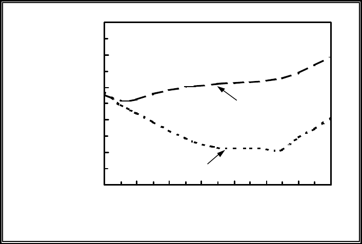
5.20

-10.0

-8.0

-6.0

-4.0

-2.0

0.0

5 6 7 8 9 10 11 12

Log Uranium Concentration (mol/l)

Schoepite

Uranophane

Figure 5.3. Maximum concentration limits calculated for total dissolved

uranium as a function of pH based on the equilibrium

solubilities of schoepite and uranophane.

5.2.5.2 Application to Evaluation of K

Values

Chemical reaction codes can be used to calculate bounding, technically-defensible maximum

concentration limits for dissolved contaminants as a function of key composition parameters

(e.g., pH) of any specified soil-water system. The concentration of a dissolved contaminant

predicted with default or site specific K

values used in transport or risk assessment models may

exceed the concentration limit based on solubility relationships. In these instances, the solubility-

limited concentration may provide a more realistic bounding value than one based on a K

value

for the assessment calculation, and could have an important impact on the estimated level of risk.

If a calculated concentration limit is based on the solubility of a mineral that is known to

precipitate under analogous chemical conditions and over reasonable time frames, then the user

knows that the dissolved concentrations of this contaminant in an actual, open soil-water system

cannot exceed these values and will most likely be significantly less than these values due to

adsorption and/or coprecipitation processes.

Moreover, as with the aqueous speciation calculations discussed in Section 5.2.3, mass transfer

calculations can be rapidly and inexpensively repeated using a chemical reaction code to determine

5.21

their sensitivity to a wide range of chemical parameters for a soil-water systems. This includes

easily measured parameters, such as pH, and analytical values that might have a wide range of

uncertainty, such as the concentration of a dissolved complexant.

5.2.6 Adsorption Submodel

The MINTEQA2 also includes a submodel to calculate the adsorption of dissolved constituents

onto the surfaces of solid phases that can be selected by the code user. The MINTEQA2 code

includes 7 adsorption model options. These are:

C Non-electrostatic adsorption models

- Activity partition coefficient (K

act

) model

- Activity Langmuir model

- Activity Freundlich model

- Ion exchange model

C Electrostatic adsorption models

- Constant capacitance model (CCM)

- Diffuse layer model (DLM)

- Triple layer models (TLM).

The equations and reactions that support these models, as coded in MINTEQA2, are described in

greater detail in Section 3. These descriptions and associated equations are adapted from

Allison et al. (1991).

The K

act

, Langmuir, and Freundlich models in MINTEQA2 are formulated in terms of species

activities, and not the more traditional approach of total concentrations of dissolved metal. In the

latter case, the total concentrations of a dissolved metal M would equal the sum of the

concentrations of all of its dissolved complexed and uncomplexed species. For example, using the

species listed in the MINTEQA2 thermodynamic database, the total concentrations of dissolved

cadmium, [Cd]

total

, in the absence of any organic complexants in the water, could include the

following species:

[Cd]

total

= [Cd

] + [CdOH

] + [Cd(OH)

(aq)] + [Cd(OH)

] +

[Cd(OH)

(aq)] + [Cd

] + [CdCO

(aq)] + [Cd(CO

)

] +

[CdHCO

] + [CdNO

] + [CdSO

(aq)] + [Cd(SO

)

] +

[CdHS

] + [Cd(HS)

(aq)] + [Cd(HS)

] + [Cd(HS)

] +

[CdCl

] + [CdCl

(aq)] + [CdCl

] + [CdOHCl

(aq)] +

[CdF

] + [CdF

(aq)] + [CdBr

] + [CdBr

(aq)] +

[CdI

] + [CdI

(aq)].

5.22

In the presence of organic complexants, [Cd]

total

could also include, in addition to the cadmium

species listed above, the concentrations of aqueous cadmium complexes containing citrate,

acetate, EDTA, HEDTA, or other organic complexes.

A total concentration approach would therefore assume that all species of metal M absorb with

equal strength. Experimental data suggest, however, that only certain aqueous species react with

the surfaces of a mineral [e.g., Waite et al. (1994)]. Based on this assumption, these non-

electrostatic models have been reformulated, as those coded in MINTEQA2, in terms of the

activities of adsorbing species to provide activity-based models. The purpose of this approach is

to reduce the dependency of the model parameters to effects from ionic strength and aqueous

complexation of the adsorbing metal by effectively allowing the adsorption of only selected

aqueous species of each metal.

Limitations remain, however, regarding these activity formulations of the K

act

, Langmuir, and

Freundlich models which restricts their range of applicability. These non-electrostatic adsorption

models do not consider: charge balance on surface sites and adsorbed species, electrostatic forces

between the adsorbing species and charge surface of the mineral, and reactions between the

mineral and dissolved constituents other than the adsorbing metal. The effect of these processes

changes with variations in the composition of an aqueous solution. These processes are,

however, incorporated into the more robust, but more data intensive, electrostatic “surface

complexation” adsorption model options in MINTEQA2.

The MINTEQA2 code includes the reaction components and formalisms necessary to enter the

required adsorption data for any of the adsorption models. The code does not however have an

adsorption database for these models. The user must provide the set of surface reactions and the

associated equilibrium constants as part of the input data set. MINTEQA2 requires that this

information be supplied relative to the adsorption of constituents onto specific mineral phases,

such as amorphous ferric hydroxide [Fe(OH)

(am)], and not a multi-mineral phase material, such

as a soil or crushed rock. Examples of MINTEQA2 input files that include the adsorption

modeling option are included in the data files distributed by EPA, and are also listed in Allison et

al. (1991 Appendix D) and Peterson et al. (1987a). These examples demonstrate the major data

requirements for some of the adsorption model options in MINTEQA2.

5.2.6.1 Examples of Modeling Studies

Modeling studies by Peterson et al. (1986), Davis and Runnells (1987), Loux et al. (1989), and

Turner et al. (1993) are examples of the use of MINTEQ adsorption model options. Peterson et

al. (1986) and Davis and Runnels (1987) studied ground-water contamination associated with

waste impoundments for uranium mill tailings using laboratory and computer modeling

techniques. Peterson et al. (1986) modeled the adsorption of arsenic, chromium, lead, selenium,

and zinc using the triple layer model (TLM) in MINTEQ. Their conceptual model was based on

the assumption that adsorption of these metals occurred only on amorphous ferric hydroxide

[Fe(OH)

(am)] that precipitated and dissolved during the course of their experiments.

5.23

Adsorption parameters for the TLM for amorphous ferric hydroxide were taken from published

sources. The results of the adsorption calculations were in good agreement with some results

from their laboratory experiments.

Davis and Runnels (1987) used MINTEQ to successfully model the behavior of zinc observed in

laboratory column experiments. They assumed that the concentration of dissolved zinc measured

in their solution samples was controlled by adsorption on amorphous ferric hydroxide

[Fe(OH)

(am)] that precipitated as a result of pH changes occurring in their experiments. The

adsorption of zinc on Fe(OH

) (am) was calculated using the TLM in MINTEQ. Davis and

Runnels describe the selection of adsorption parameters used for the TLM.

Loux et al. (1989) used the MINTEQA2 code to model the pH-dependent partitioning

of 8 cationic constituents by precipitation and/or adsorption on a sandy aquifer material in an

oxidizing environment. The constituents of interest included barium, beryllium, cadmium, copper,

nickel, lead, thallium, and zinc. Adsorption of these elements was based on amorphous iron oxide

as the only reactive adsorption surface and calculated using the diffuse layer model (DLM). The

adsorption parameters and associated reactions for the diffuse layer model were taken from

Dzombak (1986). The modeling results were compared to laboratory data for the aquifer material

spiked with the trace metals. The predicted concentrations based on the diffuse layer model for

adsorption of lead, nickel, and zinc, provided a good description of the pH behavior observed for

the spiked samples. The concentrations of the other trace metals were not adequately predicted

by the model. These differences were attributed to limitations in the model and/or available

thermochemical data.

Turner et al. (1993) used the TLM in MINTEQA2 code to model adsorption data for U(VI) on

goethite ["-FeO(OH)]. The FITEQL code was used for adsorption parameter optimization.

Their study illustrates the extensive parameter-fitting process that the user must complete to use

complex electrostatic adsorption models, such as the TLM.

5.2.6.2 Application to Evaluation of K

Values

Chemical reaction models cannot be used to predict a K

value. The user must supply the

adsorption parameters when using any of the adsorption model options. Typically, the data

required to derive the adsorption parameters needed as input for adsorption submodels in

chemical reaction codes are more extensive than information reported in a laboratory batch K

study. However, if the parameters have been determined for a particular constituent for a surface

complexation model, a chemical reaction model, such as MINTEQA2, can be used to calculate

the masses of a constituent that are dissolved or adsorbed and how changes in geochemical

conditions, such as pH, affect its adsorption behavior. The user can then derive a K

using the

calculated dissolved and adsorbed masses of the constituent.

The EPA (EPA, 1992a, 1996) has used the MINTEQA2 model and this approach to estimate K

values for several metals under a variety of geochemical conditions and metal concentrations to

5.24

support several waste disposal issues. The EPA in its “Soil Screening Guidance” determined

MINTEQA2-estimated K

values for barium, beryllium, cadmium, Cr(III), Hg(II), nickel, silver,

and zinc as a function of pH assuming adsorption on a fixed mass of iron oxide (EPA, 1996; RTI

1994). The calculations assumed equilibrium conditions, and did not consider redox potential or

metal competition for the adsorption sites. In addition to these constraints, EPA (1996) noted

that this approach was limited by the potential sorbent surfaces that could be considered and

availability of thermodynamic data. Their calculations were limited to metal adsorption on iron

oxide, although sorption of these metals to other minerals, such as clays and carbonates, is well

known.

The data needed to use surface complexation adsorption models are more extensive than those

from K

studies. More importantly, the data for surface complexation models are based on

adsorption on pure mineral phases, such as "-Al

, (-Al

, böhmite, goethite, magnetite,

lepidocrocite, ferrihydrite, SiO

, biotite, or kaolinite. Natural soils are more complicated,

commonly containing mixtures of more than 10 pure minerals and amorphous mineral coatings.

Unless a user can technically defend the assumption that the adsorption of a specific contaminant

is dominated in a specific soil-water system, for example, by goethite reactive surfaces, the user is

still left with the challenge of extrapolating these modeling results for pure mineral substrates to

complex heterogeneous soil-water systems. This issue has been and will continue to be the

subject of intensive study, but is not likely to be resolved in the short term or impact contaminant

migration and risk assessment modeling soon.

5.2.7 MINTEQA2 Databases

The MINTEQA2 model includes an extensive thermodynamic database that is integrated with the

aqueous speciation, solubility, and precipitation/dissolution submodels. The content and

equations governing the values stored in the thermodynamic database are described below.

MINTEQA2 does not have per se an integrated adsorption submodel database. The adsorption

reactions and associated model parameters are supplied by the user as part of each input file.

However, as discussed below, the current MINTEQA2 software package is supplied with a

limited data file for the diffuse layer model (DLM).

5.2.7.1 Thermodynamic Database

The MINTEQA2 thermodynamic database is considered by many to be one of the most extensive

databases for modeling the aqueous speciation and solubility of contaminants and geologically-

significant constituents (e.g., magnesium, silica, aluminum, etc.) in low-temperature, soil-water

systems. To understand the fundamental data needs for a thermodynamic database of a chemical

reaction code, the basic equations underlying the thermodynamic parameters stored in the

MINTEQA2 thermodynamic database will be reviewed in the next section. The content of the

MINTEQA2 thermodynamic database as distributed by EPA will be reviewed and then compared

relative to the priority constituents considered in the scope of work for this project.

5.25

log K°

r,T

& )G°

r,T

2.303 R T

(5.5)

)G°

r,298

' 3 )G°

f ,298

(products) & 3 )G°

f,298

(reactants) .

(5.6)

log K°

r,T

' log K°

r,298

)H°

r,298

2.303 R

(

298

) .

(5.7)

)H°

r,298

' 3 )H°

f,298

(products) & 3 )H°

f,298

(reactants) .

(5.8)

log K°

r,T

. log K°

r,298

(5.9)

5.2.7.1.1 Basic Equations

Thermodynamic data used by MINTEQA2 are stored in the form of equilibrium constants (K

,298

)

and enthalpies (heats) of reaction (ªH

,298

) for aqueous speciation, oxidation/reduction, mineral

solubility, and gas solubility reactions. The reference temperature for the MINTEQA2 database,

as with most geochemical models, is 298 K (25 °C). Equilibrium constants (log K

) may be

based on values that have been experimentally-determined or calculated from Gibbs free energies

of reaction (ªG

) units of cal/mol according to the equation:

where T = temperature in degrees Kelvin,

R = gas constant (1.9872 cal/mol·K)

Values for ªG

are calculated from published values for the Gibbs free energy of formation

(ªG

,298

) for each product and reactant in the aqueous speciation or solubility reaction by the

equation:

To calculate aqueous speciation and solubilities at temperatures other than 25°C, the equilibrium

constants are recalculated by the MINTEQA2 code to the temperature T of interest using the

van't Hoff relation:

Values for enthalpies of reaction are calculated from published enthalpy of formation values

(ªH

,298

) using the equation:

Values for ªH

,298

cannot be calculated for some reactions, because ªH

,298

values have not been

determined for 1 or more reaction products and/or reactants. In these cases, the MINTEQA2

code assumes that

Because of the limitations in using the van't Hoff relation for extrapolations over a wide range of

temperature, applications of the MINTEQA2 code are limited to temperatures less than 100°C.

5.26

5.2.7.1.2 Structure of Thermodynamic Database Files

Typically, each aqueous species, redox, mineral, and gas solubility reaction is represented by 2 fix-

formatted lines in the thermodynamic database files supplied with MINTEQA2. A third line is

sometimes included when the stoichiometry of a reaction is complex. The first file line includes

the identification number, formula descriptor, ªH

,298

(if available), log K

,298

, charge, and related

data for each reaction. The second line includes the reaction stoichiometry information

formulated in terms of the MINTEQA2 components. Each reaction is entered as a formation

reaction; that is, the components react to form the “more complex” species, such as an aqueous

complex or mineral phase. The hydrogen stoichiometric component of each reaction is balanced

with the components H

and H

O. The hydroxyl species, OH

, is not used as a component, but is

“formed” in a separate reaction in MINTEQA2.

Based on the protocol used for the MINTEQA2 thermodynamic database, the formation reaction

for the uranyl mixed hydroxide/carbonate aqueous species, (UO

)

(OH)

, is

2 UO

+ CO

+ 3 H

O = 3 H

+ (UO

)

(OH)

The corresponding entry in the MINTEQA2 database (in fixed format fields) for this reaction and

its associated thermochemical data is

8931405 UO2)2CO3OH)3 -14.3940 -0.8969 0.000 0.000-1.00 4.00 0.00 651.0868

2.00 4 2.000 893 1.000 140 3.000 2 -3.000 330

For more detailed format information on the MINTEQA2 database files, the reader is referred to

the documentation in Allison et al. (1991, Appendix A).

5.2.7.1.3 Database Components

The thermodynamic database in the original MINTEQ code (Felmy et al., 1984) was taken from

the WATEQ3 code (Ball et al., 1981a). Therefore, many of the inorganic reactions and

associated thermodynamic values in the MINTEQA2 database can be traced back to the database

supplements and sources described in publications documenting the WATEQ series of chemical

reactions codes (Ball et al., 1981a, WATEQ2; Ball et al., 1981b, WATEQ3; Plummer et al.,

1976, WATEQ; Truesdell and Jones, 1973, WATEQ; Truesdell and Jones 1974, WATEQ).

The thermodynamic database of the current version of MINTEQA2 includes the original

MINTEQ database plus modifications and additions completed on contracts with EPA funding.

Some of these supplements include, for example, those completed at PNNL, such as the addition

of reactions for aqueous species, gases, and solids containing cyanide and antimony by Sehmel

Deutsch, W. J., and K. M. Krupka. September 1985. MINTEQ Geochemical Code:

Compilation of Thermodynamic Database for the Aqueous Species, Gases, and Solids Containing

Chromium, Mercury, Selenium, and Thallium. Unpublished report prepared by Pacific Northwest

Laboratory for the U.S. Environmental Protection Agency in Athens, Georgia.

Although important to contaminant disposal and remediation activities (i.e., “mixed wastes”)

in the United States, computer modeling of the complexation of contaminant metals with organic

complexes was excluded from the scope of the current project due to funding limits.

5.27

(1989) and those containing chromium, mercury, selenium, and thallium by Deutsch and Krupka.

Documentation for these database supplements are not listed in Brown and Allison (1987,

MINTEQA1) or Allison et al. (1991, MINTEQA2), and may not be publicly available.

The elements for which the MINTEQA2 thermodynamic database has aqueous speciation, mineral

solubility, and/or gas solubility reactions are listed in Table 5.3. The second and third columns of

this table list the component species used for these elements and the redox reactions, if any,

included in MINTEQA2 for different valence states of a particular element. The reader should

note that the database does not contain reactions and associated thermodynamic values for

specific isotopes of a particular element. The calculated reactions for a soil-water system assumes

the total mass of each element.

Although the list of elements in Table 5.3 is substantial, this table and/or a listing of the database

files does not indicate if the database of a chemical reaction code, especially for key contaminants,

is adequate (i.e., completeness of reactions and quality of associated thermodynamic values) and

up-to-date. The user essentially has this important responsibility. One should expect that, as the

period of time between the publication of a code’s documentation and its use in an application

study increases, the thermodynamic database becomes dated and revisions may be warranted.

Table 5.4 lists the organic ligands for which the MINTEQA2 thermodynamic database has

aqueous speciation reactions.

Because of the limited availability of thermodynamic data for

metal-organic complexes important to contaminated soil-water systems, as compared to

inorganic aqueous complexes, the MINTEQA2 database, as with all chemical reaction codes, is

limited. It does not contain complexation reactions for all metals with each of the organic ligands

listed in Table 5.4. The reader will need to do a computer search of the MINTEQA2 ASCII file

containing these reactions to determine the extent of the organic complexation reactions for each

metal.

5.2.7.1.4 Status Relative to Project Scope

The contaminants chosen for study in this project include chromium, cadmium, cesium, tritium

(

H), lead, plutonium, radon, strontium, thorium, and uranium. Because the MINTEQA2

thermodynamic database does not contain reactions for specific isotopes, an appraisal of the

database content to aqueous speciation and solubility reactions containing tritium is not

Deutsch, W. J., and K. M. Krupka. September 1985. MINTEQ Geochemical Code:

Compilation of Thermodynamic Database for the Aqueous Species, Gases, and Solids Containing

Chromium, Mercury, Selenium, and Thallium. Unpublished report prepared by Pacific Northwest

Laboratory for the U.S. Environmental Protection Agency in Athens, Georgia.

5.28

appropriate. As will be discussed in Volume II of this report, the concentrations of dissolved

tritium will be affected by exchange reactions involving hydrogen-containing species dissolved in

the soil-water system.

Of the remaining elements, the MINTEQA2 thermodynamic database contains aqueous speciation

and solubility reactions for chromium, including the valence states Cr(II), Cr(III), and Cr(VI);

cadmium; lead; strontium; and uranium, including the valence states U(III), U(IV), U(V), and

U(VI). Except for uranium, the adequacy of the database for these listed elements is not known.

Data supplied by Deutsch and Krupka

in 1985 is the probable basis for the chromium reactions

and associated thermodynamic data. The reactions for cadmium, lead, and strontium may be

those taken from the WATEQ-series of codes and supplied with the original MINTEQ code by

Felmy et al. (1984). It is not known if these have been revised or supplemented since that time.

The reactions and associated thermodynamic data for uranium aqueous species and solid phases

were those supplied with the original MINTEQ code. They were taken from those added to

WATEQ3 (Ball et al., 1981a) and are based primarily on the compilation of uranium

thermodynamic data by Langmuir (1978). Langmuir’s review has been superseded by the

comprehensive review and compilation of uranium thermodynamic data given in Wanner and

Forrest (1992). This compilation represents a significant improvement and update to the values in

Langmuir et al. (1978), including for U(VI) carbonate and hydrolysis species that are important in

soil-water systems with pH values greater than 5.

Of the elements included in the project scope, the thermodynamic database distributed by EPA

with MINTEQA2 does not contain reactions and associated thermodynamic data for aqueous

species and solids containing cesium, plutonium, radon, and thorium. Published compilations of

thermodynamic data for aqueous species, solids, and gases containing these elements are

available, such as an Langmuir and Herman (1980), Lemire and Tremaine (1980), Peterson et al.

(1987b), Phillips et al. (1988), Smith and Martell (1976 and more recent supplements), Smith et

al. (1997), Wagman et al. (1982), and others. These sources can be used as good starting points

for adding reactions for cesium, plutonium, radon, and thorium to the MINTEQA2 database.

However, because these sources are becoming dated, additional reviews of the more recent

thermodynamic literature would be needed to supplement them and generate more up-to-date

compilations for these elements. Other compilations of thermodynamic data for these elements

include databases compiled by geochemical modeling groups elsewhere in the United States and

other countries. When documented, these databases are useful sources of information.

5.29

Table 5.3. Component species in MINTEQA2 thermodynamic database.

Element Component Species Valence States

Ag Ag

Al Al

As H

AsO

E (aq), H

AsO

E, (aq) As(III), As(V)

B H

E (aq)

Ba Ba

Br Br

C CO

, CN

, OCN

Ca Ca

Cd Cd

Cl Cl-

Cr Cr

, Cr(OH)

, CrO

Cr(II), Cr(III), Cr(VI)

Cu Cu

, Cu

Cu(I), Cu(II)

F F

Fe Fe

, Fe

Fe(II), Fe(III)

Electron e

H H

, H

O (l)

Hg Hg

, Hg(OH)

E (aq) Hg(I), Hg(II)

I I

K K

Li Li

Mg Mg

5.30

Table 5.3. Continued.

Element Component Species Valence States

Mn Mn

, Mn

Mn(II), Mn(III)

, NO

, CN

OCN

N(-III), N(III), N(V)

Na Na

Ni Ni

P PO

Pb Pb

Rb Rb

S HS

, SE, SO

S(-II), S(VI)

Sb Sb(OH)

E (aq), Sb(OH)

Sb(III), Sb(V)

Se HSe

, HSeO

, SeO

Se(-II), Se(IV), Se(VI)

Si H

SiO

E (aq)

Sr Sr

Tl Tl

, Tl(OH)

E (aq) Tl(I), Tl(III)

U U

, U

, UO

U(III), U(IV), U(V), U(VI)

V V

, V

, VO

V(II), V(III), V(IV), V(V)

Zn Zn

Center for Nuclear Waste Regulatory Analyses (CNWRA), Southwest Research Institute,

San Antonio, Texas

5.31

Table 5.4. Organic ligands in MINTEQA2 thermodynamic database.

Organic Constituents / Complexants

acetate

butyrate

iso-butyrate

citrate

diethylamine

dimethylamine

EDTA

ethylenediamine

formate

fulvate

glutamate

glycine

hexylamine

humate

iso-propylamine

n-propylamine

methylamine

2-methyl pyridine

3-methyl pyridine

4-methyl pyridine

n-butylamine

nitrilotriacetate

phthalate

propanoate

salicylate

tartrate

tri-methylamine

tributylphosphate

valerate

iso-valerate

It should be noted that the thermodynamic database distributed with EPA’s MINTEQA2 software

package does not include reactions and thermodynamic data for aqueous species and solids

containing americium, cobalt, neptunium, niobium, radium, and technetium. Although these

radionuclides are not part of the scope of this project, they may be important with respect to

contamination and remediation at some sites in the United States and/or performance assessments

of proposed LLW and HLW disposal facilities or decommissioning sites. Except for niobium,

published compilations of thermodynamic data for these elements, especially for americium (Silva

et al., 1995) and technetium (Rard, 1983), exist that can be used to supplement the MINTEQA2

database. The thermodynamic data for aqueous species and solids containing niobium are

extremely limited which precludes adequate modeling of aqueous/solid phase equilibria for

niobium in soil-water systems.

The thermodynamic database of MINTEQA2 was augmented by Krupka and Serne (1998) for

aqueous species and solids containing several radionuclide elements of interest to NRC. These

database modifications were based on data files provided by D. Turner

who had added these

5.32

reactions and thermodynamic data to his version of MINTEQA2. The database additions

included MINTEQ-formatted reactions, associated thermodynamic data (i.e., log K°

r,298

and

)H°

r,298

) and ancillary information (e.g., identification number, formula, charge, mass, reaction

stoichiometry) for aqueous species and solids containing americium, neptunium, plutonium,

radium, technetium, thorium, and uranium. The database changes for uranium are based on the

compilation by Wanner and Forest (1992), and supersede those listed in the MINTEQA2 database

as obtained from EPA. Additional revisions to the thermodynamic data for these radionuclide

elements were identified by Krupka and Serne (1998) and added to the MINTEQA2 files. These

database modifications have not undergone an in depth examination relative to quality-assurance

considerations.

5.2.7.1.5 Issues Related to Database Modifications

Successful application of chemical reaction models to quantify contaminant release and transport

in soil-water systems is dependent on the development of adequate and internally consistent

thermodynamic databases. The thermodynamic databases of chemical reaction codes are typically

revised or supplemented based on specific project needs and the availability of thermodynamic

data for aqueous species, gases, and solids containing the constituents of interest.

Although an extensive number of tabulations and critical reviews [e.g., see references in Serne et

al. (1990, Table 3.2)] of thermodynamic data for inorganic complexes and solids have been

published during the last 20 years, the selection of "best" values from these publications is a

technically and logistically challenging effort. Some of the issues and problems associated with

the selection of thermodynamic data are described in detail in Potter (1979), Nordstrom and

Munoz (1985), and Smith and Martell (1995). The critical evaluation and selection of a

thermodynamic database requires an understanding of general solution chemistry and the phase

assemblages of minerals and related amorphous solids associated with a particular cationic and/or

anionic constituent. The investigator developing the model's database

must also be cognizant of the criteria initially used to review and select the original data for the

published tabulations.

Because thermodynamic data tabulations usually contain an inadequate amount of reviewed

thermodynamic data for aqueous species of trace metals, available tabulations are typically

deficient for modeling contaminated soil-water systems. Researchers are thus faced with the

difficult responsibility of assembling thermodynamic data from other possibly less-credible

publications, borrowing values from extant chemical reaction models, and/or conducting their

own reviews of published thermodynamic data. Because there is a growing reliance on

thermodynamic review efforts completed by coworkers and other research organizations,

documentation supporting these reviews and the rationale for selecting each datum that is

“accepted” for a model's database are extremely important with respect to (1) defining the

credibility of the database, (2) achieving an internally consistent database, (3) minimizing

duplication in future review efforts, and (4) describing the selection criteria and calculation

methods used in selecting the best values.

Personal communication from N. T. Loux at the U.S. Environmental Protection Agency in

Athens, Georgia.

5.33

5.2.7.2 Sorption Database

The MINTEQA2 code is not designed to have a thermochemical database, analogous to the

thermodynamic database, that is integrated with the adsorption submodel and its 7 model options.

The adsorption reactions and associated model parameters need to be supplied by the user as part

of each input file. This process and example input files are discussed in Allison et al. (1991).

However, the current MINTEQA2/PRODEFA2 software package is supplied with a limited

adsorption data file for use with the diffuse layer adsorption model option. Data files are not

supplied for any of the other adsorption model options. The data file, formatted in ASCII, is

named FEO-DLM.dbs. It includes surface reactions and associated intrinsic conditional surface

complexation constants applicable to the diffuse layer model for the adsorption of the trace metals

, Be

, Ca

, Cd

, Cu

, Ni

, Pb

, and Zn

, and the ligands H

AsO

E (aq), H

AsO

E (aq),

E (aq), PO

, and SO

onto 2 types of iron-oxide sites. The adsorption constants are based

of data published by Dzombak (1986).

5.2.7.2.1 Status Relative to Project Scope

Of the elements chosen for study in this project, cadmium and lead are the only 2 elements

included in the diffuse layer adsorption model data file supplied with MINTEQA2. As mentioned

above, this file is restricted to adsorption onto 2 types of iron-oxide sites, and is therefore not

applicable for the adsorption of these metals to other mineral reactive surfaces. None of the other

contaminants, including chromium, cesium, plutonium, radon, strontium, thorium, or uranium, are

supported by this data file.

The MINTEQA2/PRODEFA2 software package includes no adsorption database files for the

activity partition coefficient (K

act

), activity Langmuir isotherm, activity Freundlich isotherm, ion

exchange, constant capacitance, or triple layer adsorption models.

5.2.7.2.2 Published Database Sources

No published compilations are known to exist for adsorption constants for the activity partition

coefficient (K

act

), activity Langmuir isotherm, activity Freundlich isotherm, and ion exchange

adsorption models used in MINTEQA2. Numerous individual data sets have been published for

the adsorption of many individual contaminants on specific mineral substrates, such as TiO

goethite. Typically, these data are parameterized using 1 or more of the surface complexation

models. Compilations and review of these studies was beyond the scope of this project.

Smith and Jenne (1988) (and related papers by Dzombak and Hayes, 1992, and Smith and Jenne,

1992) compiled and evaluated published values for triple layer model constants for the adsorption

5.34

of numerous constituents on "-FeO(OH), amorphous iron(III) hydrous oxide, and *-MnO

solids.

This study was conducted for the U.S. Environmental Protection Agency (Athens, Georgia) for

use in modeling the migration of contaminants in ground-water systems. Their compilation

included intrinsic constants and associated reaction stoichiometries for the adsorption of species

containing the following constituents:

C For adsorption onto Fe(III) hydrous oxides: Ag, As(V), Ba, CO

, Ca, Cd, Co, Cr(VI),

Cu(II), Fe(II), Hg(II), Mg, Mn(II), Np(V), Pb, Pu(IV), Sb(III), Sb(V), Se(VI), Se(IV), S,

, Th(I), U(VI), and Zn

C For adsorption onto *-MnO

: Ag, Ba, Ca, Cd, Co, Cu(II), Fe(II), Hg(II), Mg, Mn(II), Pb,

Th(I), and Zn.

Turner (1995) compiled and critically reviewed adsorption data reported in the literature for

surface complexation models. He then used a uniform approach to parameterize these data using

the diffuse layer, constant capacitance, and triple layer surface complexation models. His study

was conducted in support of research funded by NRC to study the potential migration of

radionuclides associated with the geologic disposal of commercial high level radioactive waste.

Turner (1993) previously described the use of the MINTEQA2 chemical reaction code to model

adsorption of radionuclides. Turner (1995) reported model constants for:

C Americium(III) on "-Al

, (-Al

, and amorphous SiO

C Neptunium(V) on "-Al

, (-Al

, boehmite ((-AlOOH), goethite ["-FeO(OH),]

magnetite (Fe

), lepidocrocite [(-FeO(OH)], ferrihydrite (5Fe

·9H

O), amorphous

SiO

, biotite mica [K(Mg,Fe)

(Al,Fe)Si

(OH,F)

], and kaolinite [Al

(OH)

]

C Plutonium(IV) on goethite

C Plutonium(V) on (-Al

and goethite

C Thorium on (-Al

and amorphous SiO

C Uranium(VI) on "-Al

, magnetite, ferrihydrite, goethite, quartz (SiO

), and kaolinite

C Carbon on ferrihydrite.

We are not aware of any other major published compilations of adsorption thermochemical data

for use with MINTEQA2. Moreover, it is very possible that individual investigators have

compiled and parameterized their own databases of adsorption constants based on the needs of

their individual research projects. General access, especially in these days of cost recovery, and

quality assurance issues will likely prohibit the use of many such individual data files.

5.35

5.3 Adsorption Model Options in MINTEQA2

The MINTEQA2 chemical reaction code includes 7 adsorption model options. Each of these

adsorption models and their associated equations and reactions are briefly described below.

MINTEQA2 includes the following non-electrostatic adsorption models

C Activity partition coefficient (K

act

) model

C Activity Langmuir model

C Activity Freundlich model

C Ion exchange model

and electrostatic adsorption models

C Diffuse layer model

C Constant capacitance model

C Triple layer models.

The following descriptions and associated equations are adapted from the MINTEQA2

documentation by Allison et al. (1991). When using the adsorption model options, readers are

cautioned to read the MINTEQA2 documentation carefully relative to correct entry and

formulation of model reactions and associated constants.

It should be noted that the non-electrostatic models in MINTEQA2 are formulated in terms of

species activities, and not the more traditional approach of total concentrations of dissolved metal.

The purpose of this approach is to reduce the dependency of the model parameters to effects from

ionic strength and aqueous complexation of the adsorbing metal.

Limitations remain, however, regarding these activity formulations which restricts the range of

applicability of these non-electrostatic models. These non-electrostatic adsorption models do not

consider: charge balance on surface sites and adsorbed species, electrostatic forces between the

adsorbing species and charged surface of the mineral, and reactions between the mineral and

dissolved constituents other than the adsorbing metal. The effect of these processes changes with

variations in the composition of an aqueous solution. These processes are, however, incorporated

into the more robust, but more data intensive, electrostatic “surface complexation” adsorption

models. The following descriptions of the electrostatic adsorption models incorporated into

MINTEQA2 are cursory. The reader is referred to sources, such as Westall and Hohl (1980),

Morel et al. (1981), Barrow and Bowden (1987), and Davis and Kent (1990), for detailed

descriptions, comparisons, and derivations of the relevant equations and reactions associated with

these models.

5.36

5.3.1 Electrostatic Versus Non-Electrostatic Models

Hydrous oxides of iron, manganese, and aluminum and amorphous aluminosilicates that exist as

discrete mineral grains or surface coatings on other minerals in soils are assumed to be primary

adsorbents for trace metals ions. These solid phases have variable surface charges and exhibit

amphoteric behavior. The solids have a net positive charge at pH values below their point of zero

charge (PZC) and a net negative charge at pH values above the PZC (see Chapter 2).

These surface charges create electrostatic potentials extending into the surrounding solutions.

Dissolved aqueous species that have a charge of the same polarity as the surface will be repelled,

while aqueous species with a charge opposite to that of the surface will be attracted (adsorbed).

The electrostatic potentials associated with charged surfaces may therefore affect the adsorption

of dissolved species on these surfaces. Unlike the non-electrostatic adsorption models, the

electrostatic models include a component that accounts for the electrostatic potentials at the

charged surface. The mass action equations of electrostatic adsorption models include terms that

modify the activities of adsorbing species approaching charged surfaces by the electrical work

necessary to penetrate the zone of electrostatic potentials (R's) associated with the mineral

surface. The 3 electrostatic models in MINTEQA2 differ primarily in the types of surface species

that are allowed within specific physical locations or layers extending away from the surface and

in the parameters that each model uses.

The 3 electrostatic models in MINTEQA2 deal with adsorption as surface complexation reactions

analogous to aqueous complexation reactions in solution. In the descriptions of the MINTEQA2

adsorption models that follow, surface sites are represented in the adsorption reactions and mass

action expressions as SOH groups, where S refers to the mineral structure and adsorption site

located at the solid-liquid interface. Some ions, such as H

, OH

, and a variety of trace metal ions

are assumed to be adsorbed by complexation with these surface sites.

In the triple layer model (TLM), the most complicated of the 3 electrostatic adsorption models in

MINTEQA2, the space around the solid surface is represented in surface complexation adsorption

models as 3 semi-infinite layers or zones between the solid surface and the solution (Figure 5.4).

These zones are separated by the o, $, and d planes. Starting at the mineral surface, The o plane

represents the first interface between the solid surface and the aqueous phase. Generally, only the

and OH

ions are allowed to penetrate the o layer to interact with the solid surface. Beyond

the o plane, farther from the mineral surface, is the $ plane which ends at the boundary of the

diffuse zone, the d plane. Dissolved ions, such as macro constituents (e.g., Na

, Ca

, and SO

)

and trace constituents ions that are adsorbing onto the solid surface are allowed into the $ layer.

The third layer is the diffuse zone where the ions are not influenced strongly by electrostatic

charge on the solid surface. The ions in this region are considered to be counterions that

neutralize any residual charge caused by the surface and adsorbed ions in the $ layer. Continuing

further from the mineral surface, the d layer blends into the bulk solution.

5.37

Distance From Surface (x)

Diffuse Layer of

Counter Ions

Schematic of

Surface Species

Schematic of

Charge-Potential

Relationships

Potential

(

)

´O´ Plane: ψ

& σ

X——O - H

X——O - ( )

X——O - H

X——O - ( )

- Cd

X——O - ( )

- CdOH

Constants

Corresponding

to Surface Species

CdOH

´b´ Plane: ψ

& σ

´d´ Plane: ψ

& σ

X——O - H

X——O - ( )

- Na

X——O - H

- Cl

X——O - H

- SO

SO4

Figure 5.4. Schematic representation of the triple layer model showing

surface species and surface charge-potential relationships.

[Taken from Peterson et al. (1987a). Brackets in the o

plane indicated deprotonated surface sites.]

5.38

Distance From Surface (x)

Diffuse Layer of Counter Ions

Schematic of

Surface Species

Schematic of

Charge-Potential

Relationships

Potential (ψ)

C´

ψ(x)

´d´ Plane or Outer

Helmholtz Plane (OH)

´O´ Plane at Potential ψ

and Charge

X——O - H

X——O - ( )

X——O - H

X——O - Cd

X——O

Constants

Corresponding

to Surface Species

Cd1

Cd2

The conceptual models for the constant capacitance (Figure 5.5) and diffuse layer models are

simplified to only 2 zones separated by the o and d planes. The difference between these

2 adsorption models is in the function relating total surface charge, T

, to surface potential R

(discussed in Sections 5.3.6 and 5.3.7). This function [R(x) in Figure 5.5)] is linear and

exponential, respectively, in the constant capacitance and diffuse layer models. It should be noted

that parameters subscripted with “o” in that 2-layer models are not equivalent to the o plane

parameters defined for the triple layer model due to differences in the definition of the o plane.

Figure 5.5. Schematic representation of the constant capacitance layer model showing

surface species and surface charge-potential relationships. [Taken from

Peterson et al. (1987a). Brackets in the o plane indicated deprotonated

surface sites.]

5.39

F % F

' 0 .

(5.10)

% F

' F

(5.11)

% F

) % F

' 0 .

(5.12)

} ' {X

}[e

&RF/RT

]

(5.13)

In all 3 models, a charge, F, associated with the surface is assumed to be balanced by a charge (F

)

associated with the diffuse layer d of counterions such that

In the constant capacitance and diffuse-layer models, all adsorbed ions contribute to the surface

charge. However, the net charge F due to adsorption in the triple layer model is the sum of the

charges associated with 2 rather than 1 adsorbing plane. These include the innermost o plane and

the $ plane, which are characterized by charges F

and F

, respectively. Thus, for the triple layer

model, the net surface charge is given by

which is balanced by the charge in the diffuse layer such that

Because the electrical potential gradients extending away from the mineral’s surface result from

the surface charge, the specifically adsorbed potential determining ions also govern distributions

of counterions in the diffuse layer.

Activities of ions in solution and near the surface are influenced by the presence of electrostatic

potentials arising from the surface charge. The activity difference between ions near the surface

and those far away is the result of electrical work required to move them across the potential

gradient between the charged surface and the bulk solution. The activity change between these

zones is related to the ion charge, z, and the electrical potential, R, near the surface and can be

expressed using the exponential Boltzmann expression,

where z = charge of ion X,

} = activity of an ion X of charge z near the surface,

} = activity of ion X in bulk solution beyond the influence of the charged surface,

-RF/RT

= Boltzmann factor,

F = Faraday constant,

R = ideal gas constant, and

T = absolute temperature in Kelvin.

The general algorithm is similar for all 3 electrostatic models in MINTEQA2. Each model is only

briefly described below. The surface reactions for the electrostatic models in MINTEQA2 are

written with the Boltzmann factor included as an reactant component with a stoichiometric factor

appropriate for the reaction. Although these electrostatically-related components are included in

the mass action equations, they are not analogous to the chemical components defined in

5.40

Amount of element sorbed on solid / solid mass

Amount of element dissolved in solution / solution volume

(5.14)

SOH % M XX SOH·M

(5.15)

[SOH·M]

[M]

total diss

(5.16)

MINTEQA2 and have no analytical totals for their input values. Their total charges are

determined from equations that are unique to each electrostatic model and potential. The activity

coefficients for the Boltzmann factor components are set to unity in MINTEQA2.

Adsorption reactions are entered as part of MINTEQA2 input files. The MINTEQA2 code, as

noted previously, has no integrated adsorption database. The adsorption reactions and associated

equilibrium constants are written in terms of the neutral surface site, SOH. They are entered as

formation reactions, analogous to the aqueous complexation and mineral solubility reactions

included in the thermodynamic database. Published adsorption reactions and associated constants

are, however, sometimes referenced to the protonated surface site SOH

for adsorbing anions and

the deprotonated site SO

for adsorbing cations. In these cases, the user must modify the

published reaction and equilibrium constant data in terms of MINTEQA2 components to use them

in a MINTEQA2 input file.

5.3.2 Activity Partition Coefficient (K

) Model

The traditional partition coefficient, K

, adsorption model (see Chapter 2) is defined as the ratio of

the concentration of metal bound on the surface of the solid to the total concentration of metal

dissolved in the liquid phase at equilibrium as in

This process can be expressed as the surface adsorption reaction

where SOH = unreacted surface site,

M = a dissolved metal M, and

SOH·M = adsorption site occupied by a component or surface-bound metal M.

The convention used for symbols in the adsorption model equations discussed in this chapter

follows that used by Allison et al.(1991). Although the basic adsorption equations are

comparable to those listed in Chapter 2, the symbols may be differ slightly.

The mass action expression for this reaction is

where [SOH·M] = concentration of adsorption sites occupied by a component M or surface-

bound metal per unit mass of adsorbing solid

5.41

act

{SOH·M}

{M}

[SOH·M]

(

[M]

(5.17)

[M]

total diss

= total concentration of dissolved M at equilibrium.

Following common convention for thermodynamic nomenclature, reaction species indicated

within [ ] refer to concentrations, and those indicated within { } refer to activities. Equation 5.16

assumes that the concentration of unreacted surface sites, SOH, are in great excess relative to the

total concentration of dissolved metal and the activity of SOH is equal to 1.

As mentioned previously, the traditional K

assumes that all species of metal M absorb with equal

strength, and [M]

total diss

includes all aqueous species containing metal M. For example, using the

species listed in the MINTEQA2 thermodynamic database, the total concentrations of dissolved

lead, [Pb]

total diss

, in the absence of any organic complexants in the water, could include the

following species:

[Pb]

total diss

= [Pb

] + [PbOH

] + [Pb(OH)

(aq)] + [Pb(OH)

] +

[Pb

] + [Pb

(OH)

] + [Pb(OH)

] +

[PbCO

(aq)] + [Pb(CO

)

] + [PbHCO

] + [PbNO

] +

[PbSO

(aq)] + [Pb(SO

)

] + [Pb(HS)

(aq)] + [Pb(HS)

] +

[PbCl

] + [PbCl

(aq)] + [PbCl

] + [PbCl

] +

[PbF

] + [PbF

(aq)] + [PbF

] + [ PbF

] +

[PbBr

] + [PbBr

(aq)] + [PbI

] + [PbI

(aq)].

In the presence of organic complexants, [Pb]

total diss

would also include, in addition to the lead

species listed above, the concentrations of aqueous lead citrate, acetate, EDTA, HEDTA, and

other organic complexes.

Because experimental data suggest that only certain aqueous species react with the surface of a

mineral, the traditional K

model is reformulated in MINTEQA2 in terms of the activities of

species to provide the activity K

act

model.

In MINTEQA2, the mass action expression for the activity K

act

model is

where {M} = free activity of the uncomplexed “bare” cation of M in the equilibrium solution,

(

= activity coefficient of dissolved species M

The quantity {SOH·M} is defined as equal to [SOH·M]. This assumption is made because there

is no generally accepted method for calculating activity coefficients for unreacted or reacted

adsorption sites. The parameter K

act

can be considered the equilibrium constant for the surface

5.42

[SOH·M] '

[SOH]

total

[M]

total diss

1 % K

[M]

total diss

(5.18)

SOH % M XX SOH·M .

(5.19)

act

{SOH·M}

{M}{SOH}

(

SOH·M

[SOH·M]

(

[M](

SOH

[SOH]

(5.20)

act

[SOH·M]

(

[M][SOH]

(5.21)

[SOH]

total

' [SOH·M] % [SOH] .

(5.22)

reaction described in Equation 5.15. This model assumes that there is an unlimited supply of

unreacted adsorption sites and the mineral surface cannot become saturated regardless of how

much M adsorbs.

5.3.3 Activity Langmuir Model

The concentration-based Langmuir adsorption model has the constraint that the number of surface

sites available for adsorption is limited. This is the only difference between the Langmuir and K

adsorption models. The partition coefficient, K

, model is linear with respect to the total

concentration of a dissolved metal, whereas the Langmuir model is non-linear. The user must

specify the concentration of available adsorption sites as part of the input file. The Langmuir

equation for adsorption is defined by

where K

= Langmuir adsorption constant,

[SOH·M] = amount of adsorbed metal M per unit mass of adsorbing solid,

[SOH]

total

= total concentration of available surface adsorption sites, and

[M]

total diss

= total concentration of dissolved metal M at equilibrium.

The surface adsorption reaction used for the Langmuir model is identical to that for the K

model

The equilibrium constant, K

act

, for this reaction can be expressed in terms of activities as

As discussed previously, the activity coefficients pertaining to unreacted and reacted surface sites

in this and the other adsorption models in MINTEQA2 are assigned values of unity.

Equation 5.20 can then be rewritten as

The mass balance equation for the available surface sites is

By combining Equations 5.21 and 5.22 in terms of [SOH]

total

and [SOH·M], one obtains the

Langmuir relationship in terms of activities

5.43

[SOH·M] '

act

[SOH]

total

(

[M]

1 % K

act

(

[M]

(5.23)

SOH % M

XX SOH·M

act

L,1

(5.24)

SOH % M

XX SOH·M

act

L,2

(5.25)

SOH % M

XX SOH·M

act

L,n

(5.26)

[M]

total diss

[SOH·M]

[SOH]

total

[M]

total diss

[SOH]

total

(5.27)

By substituting K

act

with K

and setting (

to a value of 1, Equation 5.23 reduces to the

concentration Langmuir model expressed in Equation 5.18.

To use MINTEQA2 to model competition between different metals for adsorption on the

available surface sites, one must define the separate adsorption reactions on the surface. For the

competitive Langmuir model for the competing metals M

, M

,... M

, separate reactions with

associated mass balance expressions need to be formulated using Equations 5.19-5.21 such that

Geochemical modeling and plotting techniques may be used to derive constants for the activity

Langmuir model from experimentally-measured, concentration-based K

data. One must first

determine if the concentration-based Langmuir model fits the experimental data by using the linear

form of Equation 5.18

A plot of [M]

total diss

/[SOH·M] versus [M]

total diss

will result in a straight line with the slope

1/[SOH]

total

and intercept 1/K

[SOH]

total

if the data fit the Langmuir isotherm. The value for the

concentration-based K

is obtained by dividing this slope by the intercept. Geochemical modeling

is then used to calculate the aqueous speciation of metal M for the composition of the aqueous

solution in which the K

data were determined. The K

act

value can then be derived from an

analogous plot in which the calculated activities {M} for metal M are plotted in place of the

concentration term [M].

5.44

[SOH·M] ' K

[M]

total diss

1/N

(5.28)

SOH %

M XX SOH·M .

(5.29)

act

{SOH·M}

{M}

1/N

{SOH}

(5.30)

act

[SOH·M]

{M}

1/N

(5.31)

5.3.4 Activity Freundlich Model

The concentration-based Freundlich equation for adsorption is defined by

where K

= Freundlich adsorption constant,

[SOH·M] = amount of adsorbed metal M per unit mass of adsorbing solid,

[M]

total diss

= total concentration of dissolved metal M at equilibrium, and

N = a constant.

The Freundlich equation is sometimes written with the exponent in Equation 5.28 being N instead

of 1/N. The Freundlich model assumes, like the K

adsorption model, an unlimited supply of

unreacted adsorption sites. For the special case where N equals 1, the mass action equations for

the Freundlich and K

models are identical.

The Freundlich model can be considered as a surface adsorption reaction where the stoichiometric

coefficient for the adsorbed metal M equals 1/N as in

The equilibrium constant, K

act

, for this reaction can be expressed in terms of activities as

Like the activity K

act

model, there is no mass balance on surface sites, and, assuming an excess of

sites with respect to adsorbed metal M, the concentration, [SOH], and activity {SOH}, of the

unreacted surface sites are assumed equal and set to 1. Under these conditions and assuming

{SOH·M} equals [SOH·M] as with the activity K

act

and Langmuir models, Equation 5.30

becomes

which is similar to the K

act

model except that the stoichiometric coefficient 1/N of the adsorbing

species of metal M.

An approach using geochemical modeling and plotting techniques similar to that described for the

activity Langmuir model may be used to calculate constants for the activity Freundlich model

from experimentally-measured, concentration-based K

data. One must first determine if the

Freundlich model fits the experimental data by using the logarithmic form of the Freundlich mass

action Equation 5.28

5.45

log [SOH·M] ' log K

log [M]

total diss

(5.32)

a SOH·M

% b M

' b SOH·M

% a M

(5.33)

}

{SOH·M

}

{SOH·M

}

(

]

[SOH·M

]

(

]

[SOH·M

]

(5.34)

' 0.1174 I

sinh(ZR

F/2RT)

(5.35)

If the data fit the model, a plot of log [SOH·M] versus log [M]

total diss

will result in a straight line

with the slope 1/N and intercept log K

. Geochemical modeling is then used to calculate the

aqueous speciation of metal M for the composition of the aqueous solution in which the K

data

were determined. The K

act

value can then be derived by plotting the calculated activities {M} for

the adsorbing species of metal M in place of the concentration term [M]

total diss

5.3.5 Ion Exchange Model

Ion exchange sorption is defined as the process by which a dissolved ion M

is exchanged for an

ion M

that already occupies a surface sorption site and ion M

is in turn released back into

solution. The ion exchange reaction can be expressed as

where M

= the ion initially occupying the exchange site,

= the ion replacing M

on the exchange site;

SOH·M

= surface sites occupied by ion M

SOH·M

= surface sites occupied by ion M

, and

a and b = stoichiometric coefficients.

The equilibrium constant (selectivity coefficient), K

, for the exchange reaction expressed as

The constant K

can be written in terms of concentrations by replacing activity of each species

with the product of concentration and activity coefficient. The activity coefficients for the

occupied sites, SOH·M

, are set equal to one as was assumed for the previous adsorption models

in MINTEQA2.

5.3.6 Diffuse Layer Model

For the diffuse-layer model, the total charge, T

, for plane o is calculated as

where Z = valency of the symmetrical electrolyte (which we take as unity),

I = ionic strength, and

5.46

SOH % H

X SOH

(5.36)

K '

{SOH

}

{SOH}{H

}

(5.37)

} ' {H

F/RT

(5.38)

SOH % H

% e

F/RT

X SOH

(5.39)

K '

{SOH

}

{SOH}{H

}[e

F/RT

]

(5.40)

SOH & H

X SO

(5.41)

SOH & H

& e

F/RT

X SO

(5.42)

all other parameters are defined as in Equation 5.13.

Examples of surface reactions are listed below for protonation and deprotonation reactions as

well as for a divalent cation M

. Boltzmann factors are represented in the mass action as

components.

The surface reaction and corresponding mass action expression for the protonation reaction are,

respectively,

and

where H

denotes a hydronium ion near the surface.

The activity coefficients for the surface species SOH

and SOH are assumed to be equal to unity.

The activity of H

must be corrected for the energy change required to move from the bulk

solution to the charged surface. This activity change is represented by expressing {H

} in terms

of the activity of the bulk solution hydronium ion {H

} and associated exponential Boltzmann

expression for a charge z of 1 as

Substituting this expression for {H

} in Equations 5.36 and 5.37, one obtains the following

surface reaction and mass action equation expressed in terms of the Boltzmann factor

and

The stoichiometry for the corresponding de-protonation reaction is

Substituting for {H

} as above results in the following de-protonation surface reaction and mass

action equation

5.47

K '

{SO

}{H

}[e

F/RT

]

{SOH}

. (5.43)

SOH % M

& H

X SO·M

(5.44)

K '

{SO·M

}{H

}

{SOH}{M

}

{SO·M

}{H

}[e

F/RT

]

{SOH}{M

}[e

F/RT

]

(5.45)

K '

{SO·M

}{H

}

{SOH}{M

}[e

F/RT

]

(5.46)

. C R

(5.47)

and

The stoichiometry for a surface reaction involving a multivalent species, such as a divalent cation

, is

The mass action expression for this type of adsorption reaction also includes the charge and

stoichiometry for the adsorbing ion. Substituting for {M

} and for {H

} in Equation 5.44, one

obtains the following mass action expressions

Mass action expressions for other surface reactions are formulated in a similar manner.

5.3.7 Constant Capacitance Model

The constant capacitance model is a special case of the diffuse layer model, applicable in theory

only to systems at high, constant ionic strength. The constant capacitance model is similar to the

diffuse layer model in that they both define specific adsorption of all ions on the o plane. Except

for the values of the equilibrium constants, the mass action and charge balance equations are

identical for the these 2 adsorption models. Therefore, the surface reactions and mass action

expressions described above for the diffuse layer model also apply to the constant capacitance

model.

The difference in these 2 models is in the function relating total surface charge, T

, to surface

potential R

. In the constant capacitance model, Equation 5.35 is approximated by

where C is a constant capacitance term. Although the constant capacitance and diffuse layer

models are implemented similarly, the capacitance term C is often treated as a fitting parameter

rather than as a measured characteristic of the system.

5.48

' C

& R

)

(5.48)

' C

& R

) % C

& R

)

(5.49)

' C

& R

)

(5.50)

SOH & H

% M

X (SO·M) .

(5.51)

5.3.8 Triple Layer Model

The triple layer model (Figure 5.4) includes 2 adsorbing planes instead of 1 plane as

conceptualized in the diffuse layer and constant capacitances models. As implemented in

MINTEQA2, the o plane, the inner most zone, only includes the protonation and deprotonation

(i.e., gain or loss of H

) reactions at the surface sites. The $ plane includes other specifically

adsorbed ions with charge F

and potential R

in that zone. The diffuse layer or 'd' plane, which is

the outer most zone, includes non-specifically adsorbed ions affected by R

potentials. The

capacitances between the o and $ planes and the $ and d planes are designated C

and C

respectively. The user must provide values for both capacitance terms.

The total charges, T

, T

, and T

, associated with o, $, and d planes, respectively, in the triple-

layer model are defined as

where R

= electrostatic potential at the o plane,

= electrostatic potential at the $ plane, and

= electrostatic potential at the d plane.

Surface reactions as expressed in the triple layer model differ from those used for the diffuse layer

and constant capacitance models only in that their mass action expressions include the proper

stoichiometry for the electrostatic components representing the $ and o planes. The d plane,

which as no specific adsorption, is therefore not a factor in the stoichiometry.

The surface protonation and deprotonation reactions for the triple layer model, except for their

associated equilibrium constant values, are identical to those given above for the diffuse layer

models. Examples of surface reactions and mass action expressions for the adsorption of a mono-

and divalent cations and a monovalent anion adapted from Allison et al. (1991) are given below

for the triple layer model. They show the stoichiometric coefficients for the electrostatic

components representing the $ and o planes.

The surface reaction for the adsorption of the monovalent metal cation M

5.49

} ' {H

} [e

F/RT

] (5.52)

} ' {M

} [e

F/RT

] . (5.53)

SOM & H

& e

F/RT

% M

% e

F/RT

X SO·M

(5.54)

K '

{SO·M}{H

}[e

F/RT

]

{SOH}{M

}[e

F/RT

]

(5.55)

SOH & H

% M

X (SO·M)

(5.56)

} ' {M

}[e

F/RT

]

(5.57)

SOH & H

& e

F/RT

% M

% 2e

F/RT

X SO·M

(5.58)

K '

{SO·M

}{H

}[e

F/RT

]

{SOH}{M

}[e

F/RT

]

(5.59)

SOH % A

% H

X SOH

·A .

(5.60)

In the triple layer model, H

and M

occur in the o and $ planes, respectively. Therefore,

and

Substituting these expressions into Equation 5.51, the following MINTEQA2 reaction and mass

action expression are obtained

and

The surface reaction for the adsorption of the divalent metal cation M

For the divalent cation adsorbed in the $ plane,

Substituting this expression in the reaction above gives the following MINTEQA2 reaction and

mass action expression

and

The surface reaction for the adsorption of the monovalent anion A

This reaction results in the formation of a neutral surface complex. For the anion adsorbed in the

$ plane

5.50

} ' {A

}[e

F/RT

]

. (5.61)

SOH % A

& e

F/RT

% H

% e

F/RT

X SOH

·A (5.62)

K '

{SOH

·A}[e

F/RT

]

{SOH}{A

}{H

}[e

F/RT

]

(5.63)

Substituting this into the above anion adsorption reaction, one obtains the following MINTEQA2

reaction and mass action expression

and

The formulation of reactions and mass action expressions for other adsorbing cations and anions

is similar to those examples given above.

5.4 Summary

Chemical reaction models are valuable computational tools that may be used to analyze the

macro-chemical processes (e.g., aqueous complexation, redox, solubility, and adsorption

equilibrium) affecting the composition of a soil-water system being studied in the laboratory, field

lysimeter, or field site. They also be used to provide some bounding calculations for predicting

the changes in chemistry that will result when 1 or more of these processes are imposed on a soil-

water system.

Numerous chemical reaction models exist. The MINTEQA2 computer code was developed with

EPA funding and is currently distributed by EPA in a form that executes on personal computers.

MINTEQA2 includes aqueous speciation, solubility (i.e., saturation indices),

precipitation/dissolution, and adsorption submodels. MINTEQA2's adsorption submodel includes

4 non-electrostatic [activity partition coefficient (K

act

), activity Langmuir, activity Freundlich, and

ion exchange] models and 3 electrostatic (diffuse layer, constant capacitance, and triple layer)

adsorption model options.

MINTEQA2 and other similar chemical reaction models can be used in indirect ways to support

evaluations of K

values and related contaminant migration and risk assessment modeling. These

applications include the following:

C Calculation of aqueous speciation to determine the ionic state and composition of the

dominant species for a dissolved contaminant present in a soil-water system

C Calculation of bounding, technically-defensible maximum concentration limits for

contaminants (based on solubility constraints) as a function of key composition parameters

(e.g., pH) of any specific soil-water system

5.51

C Analysis of data from laboratory measurements of K

values to determined if any solubility

limits were exceeded during the experiments.

Chemical reaction models, however, cannot be used to predict a K

value. The user must supply

the adsorption parameters when using any of the adsorption model options. However,

MINTEQA2 may be used to predict the chemical changes that result in the aqueous phase from

adsorption using any of 7 adsorption model options.

The MINTEQA2 model includes an extensive thermodynamic database that is integrated with the

aqueous speciation, solubility, and precipitation/dissolution submodels. Of the elements included

in the project scope, the thermodynamic database distributed by EPA with MINTEQA2 does not

contain reactions and associated thermodynamic data for aqueous species and solids containing

cesium, plutonium, radon, and thorium. Published compilations of thermodynamic data for

aqueous species, solids, and gases containing these elements are available that can be used as

starting points for upgrading the MINTEQA2 database to include cesium, plutonium, radon, and

thorium aqueous species and solids. MINTEQA2 does not have per se an integrated adsorption

submodel database. The adsorption reactions and associated model parameters must be supplied

by the user as part of each input file.

6.1

6.0 REFERENCES

Alberty, R. A. 1987. Physical Chemistry. Seventh Edition, John Wiley and Sons, New York,

New York.

Allison, J. D., D. S. Brown, and K. J. Novo-Gradac. 1991. MINTEQA2/PRODEFA2, A

Geochemical Assessment Model for Environmental Systems: Version 3.0 User's Manual.

EPA/600/3-91/021, U.S. Environmental Protection Agency, Athens, Georgia, March 1991.

Ames, L. L., and J. E. McGarrah. 1980. Basalt Radionuclide Distribution Coefficient

Determinations, FY1979 Annual Report. PNL-3146, Pacific Northwest Laboratory,

Richland, Washington.

Ames, L. L., J. E. McGarrah, B. A. Walker, and P. F. Salter. 1982. “ Sorption of Uranium and

Cesium by Hanford Basalts and Associated Secondary Smectite.” Chemical Geology,

35:205-225.

Ames, L. L., and D. Rai. 1978. Radionuclide Interactions with Soil and Rock Media. EPA

520/6-78-007, U.S. Environmental Protection Agency, Office of Radiation Programs, Las

Vegas, Nevada.

ASTM (American Society of Testing and Materials). 1987. “24-hour Batch-Type Measurement

of Contaminant Sorption by Soils and Sediments.” In Annual Book of ASTM Standards,

Water and Environmental Technology, Volume 11.04, pp. 163-167, Philadelphia,

Pennsylvania.

ASTM (American Society of Testing and Materials). 1988. “Determining a Sorption Constant

) for an Organic Chemical in Soil and Sediments.” In Annual Book of ASTM Standards,

Water and Environmental Technology. Volume 11.04, pp. 731-737, Philadelphia,

Pennsylvania.

Atkinson, A. 1983. “Mathematical Modeling of Leaching From Porous Nuclear Waste-Forms.”

Radioactive Waste Management and the Nuclear Fuel Cycle, 3:371-386.

Atkinson, A., K. Nelson, and T. M. Valentine. 1986. “Leach Test Characterization of Cement-

Based Nuclear Waste Forms.” Nuclear and Chemical Waste Management, 6:241-253.

Atkinson, A., and A. K. Nickerson. 1988. “Diffusion and Sorption of Cesium, Strontium, and

Iodine in Water-Saturated Cement.” Nuclear Technology, 81:100-113.

6.2

Backhus, D. A., J. N. Ryan, D. M. Groher, J. K. MacFarlane, and P. M. Gschwend. 1993.

“Sampling Colloids and Colloid-Associated Contaminants in Ground Water.” Ground Water,

31:466-479.

Baetslé, L. H. 1967. “Migration of Radionuclides in Porous Media.” In Progress in Nuclear

Energy, Series XII, Health Physics, A.M.F. Duhamel (ed.), pp. 707-730, Pergamon Press,

Elmsford, New York.

Ball, J. W., E. A. Jenne, and M. W. Cantrell. 1981a. WATEQ3: A Geochemical Model with

Uranium Added. Open-File Report 81-1183, U.S. Geological Survey, Menlo Park,

California.

Ball, J. W., and D. K. Nordstrom. 1998. “Critical Evaluation and Selection of Standard State

Thermodynamic Properties for Chromium Metal and Its Aqueous Ions, Hydrolysis Species,

Oxides, and Hydroxides.” Journal of Chemical and Engineering Data, 43:895-918.

Ball, J. W., D. K. Nordstrom, and E. A. Jenne. 1981b. Additional and Revised Thermochemical

Data and Computer Code for WATEQ2--A Computerized Chemical Model for Trace and

Major Element Speciation and Mineral Equilibria of Natural Waters. Water Resources

Investigations WRI 78-116 (second printing), U.S. Geological Survey, Menlo Park,

California.

Ball, W. P., C. H. Buehler, T. C. Harmon, D. M. Mackay, and P. V. Roberts. 1990.

“Characterization of a Sandy Aquifer Material at the Grain Scale.” Journal of Contaminant

Hydrology, 5:253-295.

Barber, L. B., II., E. M. Thurman, and D. D. Runnells. 1992. “Geochemical Heterogeneity in a

Sand and Gravel Aquifer: Effect of Sediment Mineralogy and Particle Size on the Sorption of

Chlorobenzenes.” Journal of Contaminant Hydrology, 9:35-54.

Barrow, N. J., and J. W. Bowden. 1987. “A Comparison of Models for Describing the

Adsorption of Anions on a Variable Charge Mineral Surface.” Journal of Colloid and

Interface Science, 119:236-250.

Bates, R. L., and J. A. Jackson (eds.). 1980. Glossary of Geology. American Geological

Institute, Falls Church, Virginia.

Berry, J. A. 1992a. A Review of Sorption of Radionuclides Under the Near- and Far-Field

Conditions of an Underground Radioactive Waste Repository. Part I.

DoE/HMIP/RR/92/061 (Parts I). Harwell Laboratory, Oxfordshire, United Kingdom.

6.3

Berry, J. A. 1992b. A Review of Sorption of Radionuclides Under the Near- and Far-Field

Conditions of an Underground Radioactive Waste Repository. Part II.

DoE/HMIP/RR/92/061 (Parts II). Harwell Laboratory, Oxfordshire, United Kingdom.

Berry, J. A. 1992c. A Review of Sorption of Radionuclides Under the Near- and Far-Field

Conditions of an Underground Radioactive Waste Repository. Part III.

DoE/HMIP/RR/92/061 (Parts III). Harwell Laboratory, Oxfordshire, United Kingdom.

Biggar, J. W., and D. R. Nielsen. 1962. “Miscible Displacement: II. Behavior of Tracers.” Soil

Science Society of America Journal, 26:125-128.

Bolt, G. H., and M. G. M. Bruggenwert (eds.). 1978. Soil Chemistry. A. Basic Elements.

Developments in Soil Science 5A, Elsevier Scientific Publishing Company, New York, New

York.

Bond, W. J., and P. J. Wierenga. 1990. “Immobile Water During Solute Transport in

Unsaturated Sand Columns.” Water Resources Research, 26:2475-2481.

Bosma, W. J. P., and S. E. A. T. Van der Zee. 1993. “Transport of Reacting Solute in a One-

dimensional Chemically Heterogeneous Porous Medium.” Water Resources Research,

29:117-131.

Bosma, W. J. P., S. E. A. T. Van der Zee, and C. J. Van Duijn. 1996. “Plume Development of a

Nonlinearly Adsorbing Solute in Heterogeneous Porous Formations.” Water Resources

Research, 32:1569-1584.

Bourcier, W. L. 1990. Geochemical Modeling of Radionuclide Waste Glass Dissolution Using

EQ3/6: Preliminary Results and Data Needs. UCID-21869, Lawrence Livermore National

Laboratory, Livermore, California.

Bouwer, J. 1991. “Simple Derivation of the Retardation Equation and Application to

Preferential Flow and Macrodispersion.” Ground Water, 29:41-46.

Box, G. E. P., and D. W. Behnken. 1960. “Some New Three Level Designs for the Study of

Quantitative Variables.” Technometrics, 2:455-475.

Brown, P. L., A. Haworth, S. M. Sharland, and C. J. Tweed. 1991. HARPHRQ: A Geochemical

Speciation Program Based on PHREEQE. Report NSS/R188, Harwell Laboratory, Harwell

Laboratory, Oxfordshire, United Kingdom.

Brown, D. S., and J. D. Allison. 1987. MINTEQA1, an Equilibrium Metal Speciation Model:

User's Manual. EPA/600/3-87/012, U.S. Environmental Protection Agency, Athens,

Georgia.

6.4

Brusseau, M. L. 1994. “Transport of Reactive Contaminants in Heterogeneous Porous Media.”

Reviews of Geophysics, 32:285-313.

Brusseau, M. L., and P. S. C. Rao. 1989. “Sorption Nonideality During Organic Contaminant

Transport in Porous Media.” CRC Critical Reviews in Environmental Control, 19:33-99.

Brusseau, M. L., and J. M. Zachara. 1993. “Transport of Co

in a Physically and Chemically

Heterogeneous Porous Media.” Environmental Science and Technology, 27:1937-1939.

Buck, J. W., G. Whelan, J. G. Droppo, Jr., D. L. Strenge, K. J. Castleton, J. P. McDonald,

C. Sato, and G. P. Streile. 1995. Multimedia Environmental Pollutant Assessment System

(MEPAS): Application Guidance -- Guidelines for Evaluating MEPAS Input Parameters for

Version 3.1. PNL-10395, Pacific Northwest National Laboratory, Richland, Washington.

Buddemeir, R. W., and J. R. Hunt. 1988. “Transport of Colloidal Contaminants in Groundwater:

Radionuclide Migration at the Nevada Test Site.” Applied Geochemistry, 3:535-548.

Buffle, J., D. Perret, and M. Newman. 1992. “The Use of Filtration and Ultrafiltration for Size

Fractionation of Aquatic Particles, Colloids, and Macromolecules.” In Environmental

Particles. Part II. Sampling and Characterization of Particles of Aquatic Systems, J. Buffle

and H. Van Leeuwen (eds.), pp. 171-230, Lewis Publishers, Chelsea, Michigan.

Burr, D. T., E. A. Sudicky, and R. L. Naff. 1994. “Nonreactive and Reactive Solute Transport in

Three-dimensional Heterogeneous Porous Media: Mean Displacement, Plume Spreading, and

Uncertainty.” Water Resources Research, 30:791-815.

Carter, S. L., M. M. Mortland, and W. D. Kemper. 1986. “Specific Surface.” In Methods of

Soil Analysis -- Part 1: Physical and Mineralogical Methods, A. Klute (ed.), Second

Edition, pp. 413-422, Soil Science Society of America, Madison, Wisconsin.

Carslaw, H. S., and J. C. Jaeger. 1959. Conduction of Heat in Solids. Oxford University Press,

London, England.

Chiou, Cary T., Susan E. McGroddy, and Daniel E. Kile. 1998. “Partition Characteristics of

Polycyclic Aromatic Hydrocarbons on Soils and Sediments.” Environmental Science and

Technology, 32:264-269

Cloninger, M. O., and C. R. Cole. 1981. Reference Analysis on the Use of Engineered Barriers

for Isolation of Spent Nuclear Fuel in Granite and Basalt. PNL-3530, Pacific Northwest

Laboratory, Richland, Washington.

6.5

Cloninger, M. O., C. R. Cole, and J. F. Wahburn. 1980. An Analysis on the Use of Engineered

Barriers for Geologic Isolation of Spent Fuel in a Referenced Salt Repository. PNL-3356,

Pacific Northwest Laboratory, Richland, Washington.

Coats, K. H., and B. D. Smith. 1964. “Dead-End Pore Volume and Dispersion in Porous

Media.” Society of Petroleum Engineers Journal, 4:73-84.

Cochran, G. W., and G. M. Cox. 1957. Experimental Design. Second Edition, Wiley, New

York, New York.

Codell, R. B., K. T. Key, and G. Whelan. 1982. A Collection of Mathematical Models for

Dispersion in Surface Water and Groundwater. NUREG-0868, U.S. Nuclear Regulatory

Commission, Washington, DC.

Cole, C. R., S. B. Yabusaki, and C. T. Kincaid. 1988. CFEST-SC -- Coupled Fluid, Energy, and

Solute Transport Code, SuperComputer Version. Battelle, Pacific Northwest Laboratory,

Richland, Washington.

Corapcioglu, M. Y., and S. Kim. 1995. “Modeling Facilitated Contaminant Transport of Mobile

Bacteria.” Water Resource Research, 31:2639-2647.

Cotton, F. A., and G. Wilkinson. 1972. Advanced Inorganic Chemistry, A Comprehensive Test.

Third Edition. John Wiley and Sons, Inc., New York.

Dagan, G. 1984. “Solute Transport in Heterogeneous Porous Formations.” Journal of Fluid

Mechanics, 145:151-177.

Danielsson, L. G. 1982. “On the Use of Filters for Distinguishing Between Dissolved and

Particulate Fractions in Natural Waters.” Water Research, 16:179-182.

Davies, O. L. 1954. Design and Analysis of Industrial Experiments. Hafner, New York,

New York.

Davis, J. A., and D. B. Kent. 1990. “Surface Complexation Modeling in Aqueous

Geochemistry.” In Mineral-Water Interface Geochemistry, M. F. Hochella, Jr. and

A. F. White (eds.), pp. 177-260, Reviews in Mineralogy, Volume 23, Mineralogical Society of

America, Washington, D.C.

Davis, A., and D. D. Runnells. 1987. “Geochemical Interactions Between Acidic Tails Fluid and

Bedrock: Use of the Computer Model MINTEQ.” Applied Geochemistry, 2:231-241.

6.6

Dayal, R., H. Arora, and N. Morcos. 1983. Estimation of Cesium-137 Release from

Waste/Cement Composites Using Data from Small-Scale Specimen. NUREG/CR-3382,

Nuclear Regulatory Commission, Washington, D.C.

Dean, J. A. (ed.). 1973. Lange’s Handbook of Chemistry. McGraw-Hill, New York, New

York.

Degueldre, C., G. Longworth, V. Mowlin, and P. Vilks. 1989. Grimsel Colloid Exercise. An

International Intercomparison Exercise on the Sampling and Characterization of

Groundwater Colloids. Technical Report 39, Paul Scherrer Institut-Bericht, Wurenlingen und

Villigen, Switzerland.

Delany, J. M. 1985. Reaction of Topopah Spring Tuff with J-13 Water: A Geochemical

Modeling Approach Using the EQ3/6 Reaction Path Code. UCRL-53631 DE86 013226,

Lawrence Livermore National Laboratory, Livermore, California.

Delegard, C. H., and G. S. Barney. 1983. Effects of Hanford High-Level Waste Compounds on

Sorption of Cobalt, Strontium, Neptunium, Plutonium, and Americium of Hanford Sediments.

RHO-RE-ST-1 P, Rockwell Hanford Operations, Richland, Washington.

Delegard, C. H., S. A. Gallagher, and R. B. Kasper. 1981. Saturated Column Leach Studies:

Hanford 216Z-Z-1A Sediment. RHO-SA-210, Rockwell Hanford Operations, Richland,

Washington.

Douglas, L. A. 1989. “Vermiculites.” In Minerals in Soil Environments, J. B. Dixon and

S. B. Week (eds.), Second Edition. pp. 635-674, Soil Science Society of America, Madison,

Wisconsin.

Dragun, J. 1988. Soil Chemistry of Hazardous Materials. Hazardous Materials Control

Research Institute, Silver Spring, Maryland.

Dubinin, M. M., and L. V. Radushkevich. 1947. “Equation of the Characteristic Curve of

Activated Charcoal.” Proceedings of the Academy of Sciences, Physical Chemistry Section,

U.S.S.R., 55:331-333.

Dzombak, D. A. 1986. Toward a Uniform Model for the Sorption of Inorganic Ions on Hydrous

Oxides. Ph.D. Dissertation, Massachusetts Institute of Technology, Boston, Massachusetts.

Dzombak, D. A., and K. F. Hayes. 1992. “Comment on “Recalculation, Evaluation, and

Prediction of Surface Complexation Constants for Metal Adsorption on Iron and Manganese

Oxides.”” Environmental Science and Technology, 26:1251-1253.

6.7

Elabd, H., and W. A. Jury. 1986. “Spatial Variability of Pesticide Adsorption Parameters.”

Environmental Science and Technology, 20:256-260.

EPA (U.S. Environmental Protection Agency). 1984. Uncontrolled Hazardous Waste Site

Ranking System, A User’s Manual. HW-10, U.S. Environmental Protection Agency,

Washington, D.C.

EPA (U.S. Environmental Protection Agency). 1988. Superfund Exposure Assessment Manual.

EPA/540/1-88/001, U.S. Environmental Protection Agency, Washington, D.C.

EPA (U.S. Environmental Protection Agency). 1989. Transport and Fate of Contaminants in

the Subsurface. EPA/625/4-89/019, U.S. Environmental Protection Agency, Cincinnati,

Ohio.

EPA (U.S. Environmental Protection Agency). 1991. Site Characterization for Subsurface

Remediation. EPA/625/4-91/026, Office of Research and Development, U.S. Environmental

Protection Agency, Cincinnati, Ohio.

EPA (U.S. Environmental Protection Agency). 1992a. Background Document for Finite Source

Methodology for Wastes Containing Metal. HWEP-S0040, U.S. Environmental Protection

Agency, Office of Solid Waste, Washington, D.C.

EPA (U.S. Environmental Protection Agency). 1992b. “U.S. Environmental Protection Agency,

40 CFR 300, Appendix A, Uncontrolled Hazardous Waste Site Ranking System: A User’s

Manual.” Federal Register, 47, No. 137, July 16, 1982.

EPA (U.S. Environmental Protection Agency). 1993. “Environmental Characteristics of EPA,

NRC, and DOE Sites Contaminated with Radioactive Substances.” EPA 402-R-93-011, U.S.

Environmental Protection Agency, Office of Radiation and Indoor Air (6603J), Office of Solid

Waste and Emergency Response, Washington, D.C.

EPA (U.S. Environmental Protection Agency). 1996. Soil Screening Guidance: Technical

Background Document. EPA/540/R-96/018, U.S. Environmental Protection Agency,

Washington, D.C.

EPRI (Electric Power Research Institute). 1991. Use of Batch and Column Methodologies to

Assess Utility Waste Leaching and Subsurface Chemical Attenuation. EPRI EN-7313,

Electric Power Research Institute, Palo Alto, California.

Erdal, B. R., Chairman. 1985. Workshop on Fundamental Geochemistry Needs for Nuclear

Waste Isolation. US DOE CONF8406134, National Technical Information Service,

Springfield, Virginia.

6.8

Felmy, A. R., D. C. Girvin, and E. A. Jenne. 1984. MINTEQ: A Computer Program for

Calculating Aqueous Geochemical Equilibria. EPA-600/3-84-032 (NTIS PB84-157148),

Pacific Northwest Laboratory, Richland, Washington.

Fischer, H. B., E. J. List, R. C.Y. Koh, J. Imberger, and N. H. Brooks. 1979. Mixing in Inland

and Coastal Waters. Academic Press, New York, New York.

Freeze, R. A., and J. A. Cherry. 1979. Groundwater. Prentice-Hall, Englewood Cliffs, New

Jersey.

Friedlander, G., J. W. Kennedy, and J. M. Miller. 1966. Nuclear and Radiochemistry. Second

Edition. John Wiley and Sons, Inc., New York, New York.

Freundlich, H. 1926. Colloid and Capillary Chemistry. Methuen, London, England.

Gamerdinger, A. P., D. I. Kaplan, and C. T. Resch. 1998. Uranium(VI) Sorption and Transport

in Unsaturated, Subsurface Hanford Site Sediments – Effect of Moisture Content and

Sediment Texture. PNNL-11975, Pacific Northwest National Laboratory, Richland,

Washington.

Gamerdinger, A. P., and D. I. Kaplan. 1999. “Application of a Continuous-Flow Centrifugation

Method and Determination of Heterogeneous Solute Transport in Disturbed, Unsaturated

Sediments.” Water Resources Research, (in review).

Garrels, R. M., and C. L. Christ. 1965. Solutions, Minerals, and Equilibria. Freeman, Cooper,

and Company, San Francisco, California.

Gaudet, J. P., H. Jegat, G. Vachaud, and P. J. Wierenga. 1977. “Solute Transfer, with Exchange

Between Mobile and Stagnant Water, Through Unsaturated Sand.” Soil Science Society of

America Journal, 41:665-671.

Gee, G. W., and A. C. Campbell. 1980. Monitoring and Physical Characterization of

Unsaturated Zone Transport - Laboratory Analysis. PNL-3304, Pacific Northwest

Laboratory, Richland, Washington.

Gee, G. W., A. C. Campbell, P. J. Wierenga, and T. L. Jones. 1981. Unsaturated Moisture and

Radionuclide Transport: Laboratory Analysis and Modeling. PNL-3616, Pacific Northwest

Laboratory, Richland, Washington.

Gelhar, L. W., and C. L. Axness. 1983. “Three-Dimensional Stochastic Analysis of

Macrodispersion in Aquifers.” Water Resources Research, 19:161-180.

6.9

Giles, C. H., D. Smith, and A. Huitson. 1974. “A General Treatment and Classification of the

Solute Adsorption Isotherm. I. Theoretical.” Journal of Colloid and Interface Science,

47:755-765.

Glasstone, S. 1972. Thermodynamics for Chemists. Robert E. Krieger Publishing Company,

Huntington, New York.

Goldberg, S. 1995. “Adsorption Models Incorporated into Chemical Equilibrium Models.” In

Chemical Equilibrium and Reaction Models, R. H. Loeppert, A. P. Schwab, and S. Goldberg

(eds.), pp. 75-95, Special Publication Number 42, Soil Science Society of America, Inc.,

Madison, Wisconsin.

Goltz, M. N., and P. V. Roberts. 1986. “Interpreting Organic Solute Transport Data from a

Field Experiment Using Physical Nonequilibrium Models.” Journal of Contaminant

Hydrology,1:77-93.

Grim, R. E. 1968. Clay Mineralogy. McGraw-Hill Book Company, New York, New York.

Gschwend, P. M., D. Backhus, J. K. MacFarlane, and A. L. Page. 1990. “Mobilization of

Colloids in Groundwater Due to Infiltration of Water at Coal Ash Disposal Site.” Journal of

Contaminant Hydrology, 6:307-320.

Gschwend, P. M., and M. C. Reynolds. 1987. “Monodispersed Ferrous Phosphate Colloids in an

Anoxic Groundwater Plume.” Journal of Contaminant Hydrology, 1:309-327.

Gschwend, P. M. and S. Wu. 1985. “On the Constancy of Sediment-Water Partition Coefficients

of Hydrophobic Organic Pollutants.” Environmental Science and Technology, 19:90-96.

Gu, B., and R. K. Schulz. 1991. Anion Retention in Soil: Possible Application to Reduce

Migration of Buried Technetium and Iodine. NUREG/CR-5464, U.S. Nuclear Regulatory

Commission, Washington, D.C.

Haggerty, R., and S. M. Gorelick. 1995. “Multiple-Rate Mass Transfer for Modeling Diffusion

and Surface Reactions in Media with Pore-scale Heterogeneity.” Water Resources Research,

31:2383-2400.

Hem, J. D. 1985. Study and Interpretation of the Chemical Characteristics of Natural Water.

Water Supply Paper 2254, U. S. Geological Survey, Alexandria, Virginia.

Higgins, G. H. 1959. “Evaluation of the Groundwater Contamination Hazard from Underground

Nuclear Explosives.” Journal of Geophysical Research, 64:1509-1519.

Hillel, D. 1998. Environmental Soil Physics. Academic Press, San Diego, California.

6.10

Ho, C. H., and N. H. Miller. 1986. “Formation of Uranium Oxide Sols in Bicarbonate

Solutions.” Journal of Colloid and Interface Science, 113:232-240.

Hollander, M., and D.A. Wolfe. 1973. Nonparametric Statistical Methods. Wiley, New York,

New York..

Honeyman, B. D., and P. H. Santschi. 1988. “Metals in Aquatic Systems.” Environmental

Science and Technology, 22:862-871.

Hopmans, J. W., H. Schukking, and P. J. J. F. Torfs. 1988. “Two-Dimensional Steady State

Unsaturated Water Flow in Heterogeneous Soils with Autocorrelated Soil Hydraulic

Properties.” Water Resources Research, 24:2005-2017.

INTERA (INTERA Environmental Consultants, Inc.). 1983. Geochemical Models Suitable for

Performance Assessment of Nuclear Waste Storage: Comparison of PHREEQE and

EQ3/EQ6. ONWI-473, INTERA Environmental Consultants, Inc., Houston, Texas.

Ivanovich, M., A. G. Latham, G. Longworth, and M. Gascoyne. 1992. “Applications to

Radioactive Waste Disposal Studies.” In Uranium-Series Disequilibrium. Applications to

Earth, Marine, and Environmental Systems, M. Ivanovich and R. S. Harmon (eds.),

pp. 583-630, Oxford University Press, Oxford, England.

Jackson, K. J., and W. L. Bourcier (technical organizers). 1986. Proceedings of the Workshop

on Geochemical Modeling. CONF-8609134, National Technical Information Service,

Springfield, Virginia.

Jackson, R. E., and K. J. Inch. 1989. “The In-situ Absorption of Sr-90 in a Sand Aquifer at the

Chalk River Nuclear Laboratories.” Journal of Contaminant Hydrology, 4: 27-50.

Jacobs, G. K., and S. K. Whatley (eds.). 1985. Proceedings of the Conference on the

Application of Geochemical Models to High-level Nuclear Waste Repository Assessment.

NUREG/CR-0062 (ORNL/TM-9585), Oak Ridge National Laboratory, Oak Ridge,

Tennessee.

James, R. V., and J. Rubin. 1986. “Transport of Chloride Ion in a Water-Unsaturated Soil

Exhibiting Anion Exclusion.” Soil Science Society of America Journal, 50:1142-1149.

Jardine, P. M., G. K. Jacobs, and G. V. Wilson. 1993. “Unsaturated Transport Processes in

Undisturbed Heterogeneous Porous Media: I. Inorganic Contaminants.” Soil Science

Society of America Journal, 57:945-953.

6.11

Jenne, E. A. 1977. “Trace Element Sorption by Sediments and Soils - Sites and Processes.” In

Symposium on Molybdenum in the Environment, W. Chappel and K. Petersen (eds.),

pp. 425-553, M. Dekker, Inc., New York, New York.

Jenne, E. A. (ed.). 1979. Chemical Modeling in Aqueous Systems. Speciation, Sorption,

Solubility, and Kinetics. Symposium Series 93, American Chemical Society,

Washington, D.C.

Jenne, E. A. 1981. Geochemical Modeling: A Review. PNL-3574, Pacific Northwest

Laboratory, Richland, Washington.

Jenne, E. A.. 1998a. “Adsorption of Metals by Geomedia: Data Analysis, Modeling, Controlling

Factors, and Related Issues.” In Adsorption of Metals by Geomedia. Variables,

Mechanisms, and Model Applications, E. A. Jenne (ed.), p. 2-73, Academic Press, San

Diego, California.

Jenne, E. A. 1998b. “Priorities for Future Metal Adsorption Research.” In Adsorption of Metals

by Geomedia. Variables, Mechanisms, and Model Applications, E. A. Jenne (ed.),

p. 549-560, Academic Press, San Diego, California.

Johnson, W. H., S. M. Serkiz, L. M. Johnson, and S. B. Clark. 1995. “Uranium Partitioning

Under Acidic Conditions in a Sandy Soil Aquifer.” Paper presented at the Waste

Management ‘95 Symposium, Tucson, Arizona, February 26 - March 2, 1995.

Jury, W. A., H. Elabd, and M. Resketo. 1986. “Field Study of Napropamide Movement Through

Unsaturated Soil.” Water Resources Research, 22:749-755.

Jury, W. A., W. R. Gardner, and W. H. Gardner. 1991. Soil Physics. John Wiley and Sons, Inc.

New York, New York.

Kaplan, D. I., P. M. Bertsch, and D. C. Adriano. 1995a. “Enhanced Transport of Contaminant

Metals Through an Acidic Aquifer.” Ground Water, 33:708-717.

Kaplan, D. I., P. M. Bertsch, D. C. Adriano, and W. P. Miller. 1993. “Soil-Borne Mobile

Colloids as Influenced by Water Flow and Organic Carbon.” Environmental Science and

Technology, 27:1193-1200.

6.12

Kaplan, D. I., P. M. Bertsch, D. C. Adriano, and K. A. Orlandini. 1994a. “Actinide Association

with Groundwater Colloids in a Coastal Plain Aquifer.” Radiochimica Acta, 66/67:181-187.

Kaplan, D. I., D. B. Hunter, P. M. Bertsch, S. Bajt, and D. C. Adriano. 1994b. “Application of

Synchrotron X-Ray Fluorescence Spectroscopy and Energy Dispersive X-Ray Analysis to

Identify Contaminant Metals on Groundwater Colloids.” Environmental Science &

Technology, 28:1186-1189.

Kaplan, D. I., T. L. Gervais, and K. M. Krupka. 1998. “Uranium(VI) Sorption to Sediments

Under High pH and Ionic Strength Conditions.” Radiochimica Acta, 80:201-211.

Kaplan, D. I., and R. J. Serne. 1995. Distribution Coefficient Values Describing Iodine,

Neptunium, Selenium, Technetium, and Uranium Sorption to Hanford Sediments.

PNL-10379, Supplement 1, Pacific Northwest Laboratory, Richland, Washington.

Kaplan, D. I., R. J. Serne, and M. G. Piepho. 1995b. Geochemical Factors Affecting

Radionuclide Transport Through Near and Far Fields at a Low-Level Waste Disposal Site.

PNL-10379, Pacific Northwest National Laboratory, Richland, Washington.

Kaplan, D. I., M. E. Sumner, P. M. Bertsch, and D. C. Adriano. 1996. “Chemical Conditions

Conducive to the Release of Mobile Colloids from Ultisol Profiles.” Soil Science Society of

America Journal, 60:269-274.

Karickhoff, S. W., D. S. Brown, and T. A. Scott. 1979. “Sorption of Hydrophobic Pollutants on

Natural Sediments.” Water Research, 13:231-248.

Kim, J. J. 1986. “Chemical Behavior of Transuranic Elements in Aquatic Systems.” In

Handbook on the Physics and Chemistry of the Actinides, A. J. Freeman and C. Keller (eds.),

pp. 413-455, Elsevier Science Publ., Amsterdam, Netherlands.

Kincaid, C. T., J. R. Morrey, and J. E. Rogers. 1984. Geohydrochemical Models for Solute

Migration. Volume 1: Process Description and Computer Code Selection. EPRI EA-3417,

Volume 1, Battelle, Pacific Northwest Laboratories, Richland, Washington.

Knoll, K. C. 1960. Adsorption of Strontium by Soils Under Saturated and Unsaturated Flow

Conditions. HW-67830, General Electric Company, Hanford Atomic Products Operation,

Richland, Washington.

Koltermann, C. E., and S. M. Gorelick. 1996. “Heterogeneity in Sedimentary Deposits:

A Review of Structure-Imitating, Process-Imitating, and Descriptive Approaches.” Water

Resources Research, 32:2617-2658.

6.13

Krupka, K. M., E. A. Jenne, and W. J. Deutsch. 1983. Validation of the WATEQ4

Geochemical Model for Uranium. PNL-4333, Pacific Northwest Laboratory, Richland,

Washington.

Krupka, K. M. and J. R. Morrey. 1985. MINTEQ Geochemical Reaction Code: Status and

Applications. In Proceedings of the Conference on the Application of Geochemical Models

to High-level Nuclear Waste Repository Assessment, G. K. Jacobs and S. K. Whatley (eds.),

pp. 46-53, NUREG/CR-0062 (ORNL/TM-9585), Oak Ridge National Laboratory, Oak

Ridge, Tennessee.

Krupka, K. M. and R. J. Serne. 1998. Effects on Radionuclide Concentrations by

Cement/Ground-Water Interactions in Support of Performance Assessment of Low-Level

Radioactive Waste Disposal Facilities. NUREG/CR-6377 (PNNL-11408), Pacific Northwest

National Laboratory, Richland, Washington.

LaGrega, M.D. 1994. Hazardous Waste Management. McGraw-Hill, Inc., New York,

New York.

Landström, O., C. E. Klockars, O. Persson, K. Andersson, B. Torstenfelt, B. Allard,

S. Å. Larsson, and E. L. Tullborg. 1982. “A Comparison of In-situ Radionuclide Migration

Studies in the Studsvik Area and Laboratory Measurements.” In Scientific Basis for Nuclear

Waste Management V, W. Lutze (ed.), pp. 697-706, Materials Research Society Symposia

Proceedings, Volume 11, North Holland, New York, New York.

Langmuir, D. 1978. “Uranium Solution-Mineral Equilibria at Low Temperatures with

Applications to Sedimentary Ore Deposits.” Geochimica et Cosmochimica Acta, 42:547-569.

Langmuir, D. 1997. Aqueous Environmental Geochemistry. Prentice Hall, Upper Saddle River,

New Jersey.

Langmuir, D., and J. S. Herman. 1980. “The Mobility of Thorium in Natural Waters at Low

Temperatures.” Geochimica Cosmochimica Acta 44:1753-1766.

Langmuir, I. 1918. “The Adsorption of Gases on Plane Surfaces of Glass, Mica, and Platinum.”

Journal of the American Chemical Society, 40:1361-1403.

Lehninger, A. L. 1970. Biochemistry. Worth Publishers, Inc., New York, New York.

Lemire, R. J., and P. R. Tremaine. 1980. “Uranium and Plutonium Equilibria in Aqueous

Solutions to 200°C.” Journal of Chemical and Engineering Data, 25:361-370.

Lewis, G. N., and M. Randall. 1961. Thermodynamics. Revised by K. S. Pitzer and L. Brewer,

McGraw-Hill Book Company, New York, New York.

6.14

Lewis, R. E., T. T. Jarvis, M. R. Jarvis, and G. Whelan. 1994. Eielson Air Force Base Operable

Unit 2 Baseline Risk Assessment. PNL-8752, Pacific Northwest Laboratory, Richland,

Washington.

Liang, L., J. F. McCarthy, L W. Jolley, J. A. McNabb, and T. L. Mehlhorn. 1993. “Iron

Dynamics: Observations of Transformation During Injection of Natural Organic Matter in a

Sandy Aquifer.” Geochimica et Cosmochimica Acta, 57:1987-1999.

Lindenmeier, C. W., R. J. Serne, J. L. Conca, A. T. Owen, and M. I. Wood. 1995. Solid Waste

Leach Characteristics and Contaminant-Sediment Interactions Volume 2: Contaminant

Transport Under Unsaturated Moisture Contents. PNL-10722, Pacific Northwest

Laboratory, Richland, Washington.

Lindsay, W. L., 1979. Chemical Equilibria in Soils. John Wiley and Sons, New York,

New York.

Loeppert, R. H., A. P. Schwab, and S. Goldberg (eds.). 1995. Chemical Equilibrium and

Reaction Models. Special Publication Number 42, Soil Science Society of America, Inc.,

Madison, Wisconsin.

Loux, N. T., D. S. Brown, C. R. Chafin, J. D. Allison, and S. M. Hassan. 1989. “Chemical

Speciation and Competitive Cationic Partitioning on a Sandy Aquifer Material.” Journal of

Chemical Speciation and Bioavailability, 1:111-125.

Lyman, W. J., W. F. Reehl, and D. H. Rosenblatt. 1982. Handbook of Chemical Property

Estimation Methods -- Environmental Behavior of Organic Compounds. McGraw-Hill, New

York, New York.

Mackay, D. M., W. P. Ball, and M. G. Durant. 1986. “Variability of Aquifer Sorption Properties

in a Field Experiment on Groundwater Transport of Organic Solutes: Methods and

Preliminary Results.” Journal of Contaminant Hydrology, 1:119-132.

McCarthy, J. F., and D. Degueldre. 1993. “Sampling and Characterization of Colloids and

Particles in Groundwater for Studying their Role in Contaminant Transport.” In

Environmental Particles, J. Buffle and J. P. van Leeuwen (eds.), pp. 247-315. Lewis

Publishers, Boca Raton, Florida.

McDonald, M. G., and A. W. Harbaugh. 1988. A Modular Three-Dimensional Finite-

Difference Groundwater Flow Model. U.S. Geological Survey Techniques of Water

Resources Investigations, Book 6, Chapter A1, U.S. Geological Survey, Reston, Virginia.

6.15

McKinley, I. G., and W. R. Alexander. 1993. “Assessment of Radionuclide Retardation: Uses

and Abuses of Natural Analogue Studies.” Journal of Contaminant Hydrology, 13:249-259.

McKinley. J. P., and E. A. Jenne. 1991. <Experimental Investigation and Review of the “Solids

Concentration” Effect in Adsorption Studies.’ Environmental Science and Technology,

25:2082-2087.

McMahon, M. A., and J. W. Thomas. 1974. “Chloride and Tritiated Water Flow in Disturbed

and Undisturbed Soils Cores.” Proceedings Soil Science Society of America, 38:727-732.

Meier, H., E. Zimmerhacki, G. Zeitler, P. Menge, and W. Hecker. 1987. “Influence of

Liquid/Solid Ratios in Radionuclide Migration Studies.” Journal of Radioanalytical and

Nuclear Chemistry, 109:139-151.

Melchior, D. C., and R. L. Bassett (eds.). 1990. Chemical Modeling in Aqueous Systems II.

Symposium Series 416, American Chemical Society, Washington, D.C.

Mercer, J. W., C. R. Faust, W. J. Miller, and F. J. Pearson, Jr. 1981. Review of Simulation

Techniques for Aquifer Thermal Energy Storage (ATES). PNL-3769, Pacific Northwest

Laboratory, Richland, Washington.

Mills, W. B., S. Liu, and F. K. Fong. 1991. “Literature Review and Model (COMET) for

Colloid/Metals Transport in Porous Media.” Ground Water, 29:199-208.

Morel, F. M. M. 1983. Principles of Aquatic Chemistry. John Wiley and Sons, New York, New

York.

Morel, F. M. M., and J. G. Hering. 1993. Principles and Applications of Aquatic Chemistry.

John Wiley and Sons, Inc., New York, New York.

Morel, F. M. M., J. G. Yeasted, and J. C. Westall. 1981. “Adsorption Models:

A Mathematical Analysis in the Framework of General Equilibrium Calculations.” In

Adsorption of Inorganics at Solid-Liquid Interfaces, M. A. Anderson and A. J. Rubin (eds.),

pp. 263-294, Ann Arbor Science Publishers, Inc., Ann Arbor, Michigan.

Morrey, J. R., C. T. Kincaid, and C. J. Hostetler. 1986. Geohydrochemical Models for Solute

Migration. Volume 3: Evaluation of Selected Computer Codes. EPRI EA-3417, Volume 3,

Battelle, Pacific Northwest Laboratories, Richland, Washington.

Mucciardi, A. N., I. J. Booker, E. C. Orr, and D. Cleveland. 1979. “Statistical Investigation of

the Mechanics Controlling Radionuclide Sorption, Part II.” In Second Contractor

Information Meeting. Task 4. R. J. Serne (ed.), Vol. 2, pp 333-425, PNL-SA-7352, Pacific

Northwest Laboratory, Richland, Washington.

6.16

Mucciardi, A. N., T. C. Johnson, and J. Saunier. 1980. “Statistical Investigation of the

Mechanics Controlling Radionuclide Sorption, Part III.” In Third Contractor Information

Meeting. Task 4, J. F. Relyea (ed.), Vol. 1, pp. 1-75, PNL-SA-8571, Pacific Northwest

Laboratory, Richland, Washington.

Muller, A. B., D. Langmuir, and L. E. Duda. 1983. “The Formulation of an Integrated Physico-

chemical-Hydrologic Model for Predicting Waste Nuclide Retardation in Geologic Media.” In

Scientific Basis for Nuclear Waste Management VI, D. G. Brookins (ed.), pp. 547-564,

Materials Research Society Symposia Proceedings, Volume 15, North Holland, New York,

New York.

Nielsen, D. R., and J. W. Biggar. 1961. “Miscible Displacement in Soils: I. Experimental

Information.” Soil Science Society of America Journal, 25:1-5.

Nielsen, D. R., and J. W. Biggar. 1962. “Miscible Displacement in Soils: II. Behavior of

Tracers.” Proceedings Soil Science Society of America, 26:125-128.

Nielsen, D. R., J. W. Biggar, and K. T. Erh. 1973. “Spatial Variability of Field-Measured Soil-

Water Properties.” Hilgardia, 42:215-259.

Nielsen, D. R., M. T. van Genuchten, and J. W. Biggar. 1986. “Water Flow and Solute

Transport Processes in the Unsaturated Zone.” Water Resources Research, 22:895-1085.

Nordstrom, D. K., and J. W. Ball. 1984. “Chemical Models, Computer Programs and Metal

Complexation in Natural Waters.” In Complexation of Trace Metals in Natural Waters,

C. J. M. Kramer and J. C. Duinker (eds.), pp. 149-169, Martinus Nijhoff/Dr. J. W. Junk

Publishing Co., Netherlands.

Nordstrom, D. K., and J. L. Munoz. 1985. Geochemical Thermodynamics. The

Benjamin/Cummings Publishing Co., Inc., Menlo Park, California.

Nordstrom, D. K., L. N. Plummer, T. M. L. Wigley, T. J. Woley, J. W. Ball, E. A. Jenne, R. L.

Bassett, D. A. Crerar, T. M. Florence, B. Fritz, M. Hoffman, G. R. Holdren, Jr., G. M. Lafon,

S. V. Mattigod, R. E. McDuff, F. Morel, M. M. Reddy, G. Sposito, and J. Thrailkill. 1979.

“Comparison of Computerized Chemical Models for Equilibrium Calculations in Aqueous

Systems.” In Chemical Modeling in Aqueous Systems. Speciation, Sorption, Solubility, and

Kinetics, E. A. Jenne (ed.), pp. 857-892, American Chemical Society Symposium Series 93,

Washington, D.C.

6.17

O’Conner, D. J., and J. P. Connolly. 1980. “The Effect of Concentration of Adsorbing Solids on

the Partition Coefficient.” Water Research, 14:1517-1523.

Oscarson, D. W., and H. B. Hume. 1998. “Effect of Solid:Liquid Ratio on the Sorption of Sr

and Cs

on Bentonite.” In Adsorption of Metals by Geomedia. Variables, Mechanisms, and

Model Applications, E. A. Jenne (ed.), p. 277-289, Academic Press, San Diego, California.

Papelis, C., K. F. Hayes, and J. O. Leckie. 1988. HYDRAQL: A Program for the Computation

of Chemical Equilibrium Composition of Aqueous Batch Systems Including Surface-

Complexation Modeling of Ion Adsorption at the Oxide/Solution Interface. Technical Report

No. 306, Department of Civil Engineering, Stanford University, Stanford, California.

Parsons, R. 1982. “Surface Properties of Oxides.” Journal of Electroanalytical Chemistry,

118:2-18.

Peck, A. J., R. J. Luxmoore, and J. L. Stolzy. 1977. “Effects of Spatial Variability of Soil

Hydraulic Properties in Water Budget Modeling.” Water Resources Research, 13:348-354.

Penrose, W. R., W. L. Plozer, W. H. Essington, D. M. Nelson, and K. A. Orlandini. 1990.

“Mobility of Pu and Am Through a Shallow Aquifer in a Semiarid Region.” Environmental

Science & Technology, 24:228-234.

Petersen, L. W., P. Moldrup, O. H. Jacobsen, and D. E. Rolston. 1996. “Relations Between

Specific Surface Area and Soil Physical and Chemical Properties.” Soil Science, 161:9-21.

Peterson, R. G., and L. D. Calvin. 1986. “Sampling.” In Methods of Soil Analysis, Part 1.

Physical and Mineralogical Methods, A. Klute (ed.), American Society of Agronomy, Inc.,

Madison, Wisconsin.

Peterson, S. R., C. J. Hostetler, W. J. Deutsch, and C. E. Cowan. 1987a. MINTEQ User's

Manual. NUREG/CR-4808 (PNL-6106), Pacific Northwest Laboratory, Richland,

Washington.

Peterson, S. R., W. J. Martin, and R. J. Serne. 1986. Predictive Geochemical Modeling of

Contaminant Concentrations in Laboratory Columns and in Plumes Migrating from

Uranium Mill Tailings Waste Impoundments. NUREG/CR-4520 (PNL-5788), prepared by

the Pacific Northwest Laboratory, Richland, Washington.

Peterson, S. R., B. E. Opitz, M. J. Graham, and L. E. Eary. 1987b. An Overview of the

Geochemical Code MINTEQ: Application to Performance Assessment for Low-Level

Wastes. PNL-6112, Pacific Northwest Laboratory, Richland, Washington.

6.18

Phillips, S. L., F. V. Hale, L. F. Silvester, and M. D. Siegel. 1988. Thermodynamic Tables for

Nuclear Waste Isolation. Aqueous Solutions Database. NUREG/CR-4864 (LBL-22860),

Volume 1, Lawrence Berkeley Laboratory, Lawrence, California.

Pickens, J. F., R. E. Jackson, K. J. Inch, and W. F. Merritt. 1981. “Measurement of Distribution

Coefficients Using a Radial Injection Dual-Tracer Test.” Water Resources Research, 17:529-

544.

Pignatello, J. J. 1989. “Sorption Dynamics of Organic Compounds in Soils and Sediments.” In

Reactions and Movement of Organic Chemicals in Soils, B. L. Sawhney and K. Brown

(eds.), pp. 45-80. SSSA Special Publication 22, Soil Science Society of America, Inc.,

Madison, Wisconsin..

Plackett, R. L., and J. P. Burman. 1946. “The Design of Optimum Multifactorial Experiments.”

Biometrika, 33:305-325.

Plummer, L. N., B. F. Jones, and A. H. Truesdell. 1976, WATEQF - A FORTRAN IV Version of

WATEQ, A Computer Program for Calculating Chemical Equilibrium of Natural Waters.

Water Resources Investigations WRI 76-13, U.S. Geological Survey, Reston, Virginia.

Potter, R. W., III. 1979. "Computer Modeling in Low Temperature Geochemistry." Reviews of

Geophysics and Space Physics, 17:850-860.

Powell, R. M., and R. W. Puls. 1993. “Passive Sampling of Groundwater Monitoring Wells

Without Purging: Multilevel Well Chemistry and Tracer Disappearance.” Journal of

Contaminant Hydrology, 12:51-77.

Puls, R. W. 1990. “Colloidal Consideration in Groundwater Sampling and Contaminant

Transport Predictions.” Nuclear Safety, 31:58-65.

Rai, D., A. R. Felmy, and J. L. Ryan. 1990. “Uranium(IV) Hydrolysis Constants and Solubility

Product of UO

·xH

O(am).” Inorganic Chemistry, 29:260-254.

Rai, D., and J. M. Zachara. 1984. Chemical Attenuation Rates, Coefficients, and Constants in

Leachate Migration. Volume 1: A Critical Review. EPRI EA-3356, Volume 1, Electric

Power Research Institute, Palo Alto, California.

Rancon, D. 1973. “The Behavior in Underground Environments of Uranium and Thorium

Discharged by the Nuclear Industry.” In Environmental Behavior of Radionuclides Released

in the Nuclear Industry. IAEA-SM-172/55, pp. 333-346, International Atomic Energy

Agency, Vienna, Austria.

6.19

Rard, J. A. 1983. Critical Review of the Chemistry and Thermodynamics of Technetium and

Some of its Inorganic Compounds and Aqueous Species. UCRL-53440, Lawrence Livermore

National Laboratory, Livermore, California.

Read, D, P. J. Hooker, M. Ivanovich, and A. E. Milodowski. 1991. “A Natural Analogue Study

of an Abandoned Uranium Mine in Cornwall, England.” Radiochimica Acta, 52/53:349-356.

Reichle, R., W. Kinzelbach, and H. Kinzelbach. 1998. “Effective Parameters in Heterogeneous

and Homogeneous Transport Models with Kinetic Sorption.” Water Resources Research,

34:583-594.

Relyea, J. F. 1982. “Theoretical and Experimental Considerations for the Use of the Column

Method for the Use of the Column Method for Determining Retardation Factors.”

Radioactive Waste Management and the Nuclear Fuel Cycle, 3(2):151-166.

Ritger, P. D., and N. J. Rose. 1968. Differential Equations with Applications. McGraw Hill,

New York, New York.

Robin, M. J. L., E. A. Sudicky, R. W. Gillham, and R. G. Kachanoski. 1991. “Spatial Variability

of Strontium Distribution Coefficients and Their Correlation with Hydraulic Conductivity in

the Canadian Forces Base Borden Aquifer.” Water Resources Research, 27:2619-2632.

Routson, R. C., and R. J. Serne. 1972. One-Dimensional Model of the Movement of Trace

Radioactive Solute Through Soil Columns - The PERCEL Model. BNWL-1718, Pacific

Northwest Laboratory, Richland, Washington.

Routson, R. C., G. S. Barney, R. H. Smith, C. H. Delegard, and L. Jensen. 1981. Fission

Product Sorption Parameters for Hanford 200-Area Sediment Types. RHO-ST-35, Rockwell

Hanford Operations, Richland, Washington.

Roy, W. R., I. G. Drapac, S. F. J. Chou, and R. A. Griffin. 1991. Batch-type Procedures for

Estimating Soil Adsorption of Chemicals. EPA/530-SW-87-006-F, Office of Solid Waste and

Emergency Response, U.S. Environmental Protection Agency, Washington, D.C.

RTI (Research Triangle Institute). 1994. Chemical Properties for Soil Screening Levels. Draft

Report. Prepared for the Environmental Protection Agency, Office of Emergency and

Remedial Response, Washington, D.C.

Russo, D. 1989a. “Field-Scale Transport of Interacting Solutes Through the Unsaturated Zone

2. Analysis of the Spatial Variability of the Field Response.” Water Resources Research,

25:2487-2495.

6.20

Russo, D. 1989b. “Field-Scale Transport of Interacting Solutes Through the Unsaturated Zone

1. Analysis of the Spatial Variability of the Transport Properties.” Water Resources

Research, 25:2475-2485.

Ryan, J. M., and P. M. Gschwend. 1990. “Colloid Mobilization in Two Atlantic Coastal Plain

Aquifers: Field Studies.” Water Resources Research, 26:307-322.

Salter, P. F., L. L. Ames, and J. E. McGarrah. 1981a. The Sorption Behavior of Selected

Radionuclides on Columbia River Basalts. RHO-BWI-LD-48, Rockwell Hanford

Operations, Richland, Washington.

Salter, P. F., L. L. Ames, and J. E. McGarrah. 1981b. Sorption of Selected Radionuclides on

Secondary Minerals Associated with the Columbia River Basalts. RHO-BWI-LD-43,

Rockwell Hanford Operations, Richland, Washington.

Schindler, P. W., and G. Sposito. 1991. “Surface Complexation at (Hydro)oxide Surfaces.” In

Interactions at the Soil Colloid-Soil Solution Interface, G. H. Bolt, M. F. DeBoodt, M. H. B.

Hayes, and M. B. Mc Bride (eds.), pp. 115-145, Kluwer Academic Press, New York,

New York.

Schwarzenbach, R. P., and J. Westall. 1981. “Transport of Nonpolar Organic Compounds from

Surface Water to Groundwater. Laboratory Sorption Studies.” Environmental Science and

Technology, 15:1360-1367.

Scott, H. D., R. E. Phillips, and R. F. Paetzold. 1974. “Diffusion of Herbicides in One Adsorbed

Phase.” Proceedings Soil Science Society of America, 38:558-562.

Seaman, J. C., P. M. Bertsch, and W. P. Miller. 1995. “Ionic Tracer Movement Through Highly

Weathered Sediments.” Journal of Contaminant Hydrology, 20:127-143.

Sehmel, G. A. 1989. Cyanide and Antimony Thermodynamic Database for the Aqueous Species

and Solids for the EPA-MINTEQ Geochemical Code. PNL-6835, Pacific Northwest

Laboratory, Richland, Washington.

Sergeyeva, E. I., A. A. Nikitin, I. L. Khodakovskiy, and G. B. Naumov. 1972. “Experimental

Investigation of Equilibria in the System UO

-CO

-H

O in 25-200

C Temperature Interval.”

Geochemistry International, 9:900-910.

Serkiz, S. M. And W. H. Johnson. 1994. Uranium Geochemistry in Soil and Groundwater at

the F and H Seepage Basins (U). EPD-SGS-94-307, Westinghouse Savannah River

Company, Savannah River Site, Aiken, South Carolina.

6.21

Serne, R. J., R. C. Arthur, and K. M. Krupka. 1990. Review of Geochemical Processes and

Codes for Assessment of Radionuclide Migration Potential at Commercial LLW Sites.

NUREG/CR-5548 (PNL-7285), Pacific Northwest Laboratory, Richland, Washington.

Serne, R. J., and A. B. Muller. 1987. “A Perspective on Adsorption of Radionuclides onto

Geologic Media.” In The Geological Disposal of High Level Radioactive Wastes,

D. G. Brookins (ed.), pp. 407-443, Theophrastus Publications, S.A., Athens, Greece.

Serne, R. J., and J. F. Relyea. 1981. “The Status of Radionuclide Sorption-Desorption Studies

Performed by the WRIT Program.” In The Technology of high-Level Nuclear Waste

Disposal, Volume 1, pp. 203-254, DOE/TIC-621, Technical Information Center,

U.S. Department of Energy, Oak, Ridge, Tennessee.

Serne, R. J., R. C. Routson, and D. A. Cochran. 1973. Experimental Methods for Obtaining

PERCOL Model Input Verification Data. BNWL-1721, Pacific Northwest Laboratory,

Richland, Washington.

Seth, Rajesh, Donald MacKay, and Jane Muncke. 1999. “Estimating the Organic Carbon Partition

Coefficient and its Variability for Hydrophobic Chemicals.” Environmental Science and

Technology, 33:2390-2394.

Sheppard, J. C., J. A. Kittrick, and T. L. Hart. 1976. Determination of Distribution Ratios and

Diffusion Coefficients of Neptunium, Americium, and Curium in Soil-Aquatic Environments.

RTO-221-T-12-2, Rockwell Hanford Operations, Richland, Washington.

Sheppard, S. C., M. I. Sheppard, and W. G. Evenden. 1990. “A Novel Method Used to Examine

Variation in Tc Sorption Among 34 Soils, Aerated and Anoxic.” Journal of Environmental

Radioactivity, 11:215.

Silva, R. J., G. Bidoglio, M. H. Rand, P. B. Robourch, H. Wanner, and I. Puigdomenech. 1995.

Chemical Thermodynamics Series, Volume 2: Chemical Thermodynamics of Americium.

Elsevier Science, New York, New York.

Smith, R. M., and A. E. Martell. 1976. Critical Stability Constants. Volume 4: Inorganic

Complexes. Plenum Press, New York, New York.

Smith, R. M., and A. E. Martell. 1995. “The Selection of Critical Stability Constants.” In

Chemical Equilibrium and Reaction Models, R. H. Loeppert, A. P. Schwab, and S. Goldberg

(eds.), Special Publication Number 42, Soil Science Society of America, Inc., Madison,

Wisconsin.

Smith, R. M., A. E. Martell, and R. J. Motekaitis. 1997. NIST Critically Selected Stability

Constants of Metal Complexes Database. Version 4. Users Guide. NIST Standard

6.22

Reference Database 46, National Institute of Standards and Technology, Gaithersburg,

Maryland.

Smith, R. W., and E. A. Jenne. 1991. “Recalculation, Evaluation, and Prediction of Surface

Complexation Constants for Metal Adsorption on Iron and Manganese Oxides.”

Environmental Science and Technology, 25:525-531.

Smith, R. W. and E. A. Jenne. 1992. “Response to ‘Comment on “Recalculation, Evaluation,

and Prediction of Surface Complexation Constants for Metal Adsorption on Iron and

Manganese Oxides.’” Environmental Science and Technology, 26:1253-1254.

Smith, R. W. and E. A. Jenne. 1991. “Recalculation, Evaluation, and Prediction of Surface

Complexation Constants for Metal Adsorption on Iron and Manganese Oxides.”

Environmental Science and Technology, 25:525-531.

Smith, R. W. and E. A. Jenne. 1988. Compilation, Evaluation, and Prediction of Trip-Layer

Model Constants for Ions on Fe(III) and Mn(IV) Hydrous Oxides. PNL-6754, Pacific

Northwest Laboratory, Richland, Washington.

Snedecor, G. W., and W. G. Cochran. 1967. Statistical Methods. Sixth Edition, Iowa State

University Press, Ames, Iowa.

Sposito, G. 1984. The Surface Chemistry of Soils. Oxford University Press, New York,

New York.

Sposito, G. 1989. The Chemistry of Soils. Oxford University Press, New York, New York.

Sposito, G. 1994. Chemical Equilibria and Kinetics in Soils. Oxford University Press, New

York, New York.

Sposito, G., and J. Coves. 1988. SOILCHEM: A Computer Program for the Calculation of

Chemical Speciation in Soils. Kearny Foundation for Soil Science, University of California,

Riverside, California.

SSSA (Soil Science Society of America). 1997. Glossary of Soil Science Terms. Soil Science

Society of America, Madison, Wisconsin.

Strenge, D. L., and S. R. Peterson. 1989. Chemical Data Bases for the Multimedia

Environmental Pollutant Assessment System (MEPAS): Version 1. PNL-7145, Pacific

Northwest Laboratory, Richland, Washington.

Stumm, W. (ed.). 1987. Aquatic Surface Chemistry. Chemical Processes at the Particle-Water

Interface. John Wiley and Sons, New York, New York.

6.23

Stumm, W., and J. J. Morgan. 1981. Aquatic Chemistry. An Introduction Emphasizing

Chemical Equilibria in Natural Waters. John Wiley and Sons, New York, New York.

Sudicky, E. A. 1986. “A Natural Gradient Experiment on Solute Transport in a Sand Aquifer:

Spatial Variability of Hydraulic Conductivity and its Role in the Dispersion Process.” Water

Resources Research, 22:2069-2082.

Sugita, F., R. W. Gillham, and C. Mase. 1995. “Pore Scale Variation in Retardation Factor as a

Cause of Nonideal Reactive Breakthrough Curves. 2. pore Network Analysis.” Water

Resources Research, 31:113-119.

Szecsody, J. E., A. Chilakapati, J. M. Zachara, and A. L. Garvin. 1998. “Influence of Iron Oxide

Inclusion Shape on Co II/III EDTA Reactive Transport Through Spatially Heterogeneous

Sediment.” Water Resources Research, 34:2501-2514.

Szecsody, J. E., J. M. Zachara, and P. L. Bruckhart. 1994. “Adsorption-dissolution Reactions

Affecting the Distribution and Stability of Co (II) EDTA in Iron Oxide-Coated Sand.”

Environmental Science and Technology, 28(9):1706-1716.

Szecsody, J. E., J. M. Zachara, A. Chilakapati, P. M. Jardine, and A. S. Ferrency. 1998.

“Importance of Flow and Particle-Scale Heterogeneity on Co II/III EDTA Reactive

Transport.” Journal of Hydrology, 209:112-136.

Tompson, A.F.B., A. L. Schafer, and R.W. Smith. 1996. “Impacts of Physical and Chemical

Heterogeneity on Contaminant Transport in a Sandy Porous Medium.” Water Resources

Research, 32:801-818.

Tompson, A. F. B. 1993. “Numerical Simulation of Chemical Migration in Physically and

Chemically Heterogeneous Porous Media.” Water Resources Research, 29:3709-3726.

Tompson, A. F. B., and L. W. Gelhar. 1990. “Numerical Simulation of Solute Transport in

Three-Dimensional Randomly Heterogeneous Porous Media.” Water Resources Research,

26:2541-2562.

Truesdell, A. H., and B. F. Jones. 1973. WATEQ, A Computer Program for Calculating

Chemical Equilibria of Natural Waters. USGS-WRD-73-007, U.S. Geological Survey,

Washington, D.C.

Truesdell, A. H., and B. F. Jones. 1974. “WATEQ, A Computer Program for Calculating

Chemical Equilibria of Natural Waters.” U.S. Geological Survey Journal of Research,

2:233-248.

6.24

Turner, D. R. 1991. Sorption Modeling for High-level Waste Performance Assessment:

A Literature Review. CNWRA 91-011, Center for Nuclear Waste Regulatory Analysis, San

Antonio, Texas.

Turner, D. R. 1993. Mechanistic Approaches to Radionuclide Sorption Modeling.

CNWRA 93-019, Center for Nuclear Waste Regulatory Analysis, San Antonio, Texas.

Turner, D. R. 1995. Uniform Approach to Surface Complexation Modeling of Radionuclide

Sorption. CNWRA 95-001, Center for Nuclear Waste Regulatory Analysis, San Antonio,

Texas.

Turner, D. R., T. Griffin, and T. B. Dietrich. 1993. “Radionuclide Sorption Modeling Using

the MINTEQA2 Speciation Code.” In Scientific Basis for Nuclear Waste Management XVI,

C. G. Interrante and R. T. Pabalan (eds.), pp. 783-789, Materials Research Society

Symposium Proceedings, Volume 294, Materials Research Society, Pittsburgh, Pennsylvania.

van Genuchten, M. Th., and W. J. Alves. 1982. Analytical Solutions of the One-Dimensional

Convective-Dispersive Solute Transport Equation. Technical Bulletin No. 1661, U.S.

Department of Agriculture, Washington, D.C.

van Genuchten, M. Th., and P. J. Wierenga. 1976. “Mass Transfer Studies in Sorbing Porous

Media. I. Analytical Solutions.” Soil Science Society of America Journal, 40:473-480.

van Genuchten, M. Th., and P. J. Wierenga. 1986. “Solute Dispersion Coefficients and

Retardation Factors.” In Methods of Soil Analysis -- Part 1: Physical and Mineralogical

Methods, A. Klute (ed.), Second Edition, Chapter 44, pp. 1025-1054, Soil Science Society of

America, Madison, Wisconsin,

Voice, T. C., C. P. Rice, and W. J. Weber. 1983. “Effect of Solids Concentration on the

Sorptive Partitioning of Hydrophobic Pollutants in Aquatic Systems.” Environmental Science

and Technology, 17:513-518.

Wagman, D. D., W. H. Evans, V. B. Parker, R. H. Shumm, I. Halow, S. M. Bailey, K. L.

Churney, and R. L. Nuttall. 1982. “The NBS Tables of Chemical Thermodynamic Properties.

Selected Values for Inorganic and C1 and C2 Organic Substances in SI Units.” Journal of

Physical and Chemical Reference Data 11(Supplement No. 2):1-392.

Waite, T. D., J. A. Davis, T. E. Payne, G. A. Waychunas, and N. Xu. 1994. “Uranium(VI)

Adsorption to Ferrihydrite: Application of a Surface Complexation Model.” Geochimica et

Cosmochimica Acta, 58(24):5465-5478.

Wanner, H, and I. Forest (eds.). 1992. Chemical Thermodynamics Series, Volume 1: Chemical

Thermodynamics of Uranium. (I. Grenthe, J. Fuger, R. J. M. Konings, R. J. Lemire, A. B.

6.25

Muller, C. Nguyen-Trung, and H. Wanner, review team), North-Holland, Elsevier Science

Publishing Company, Inc., New York, New York.

Warrick, A. W., and A. Amoozegar-Fard. 1979. “Infiltration and Drainage Calculation Using

Spatially Scaled Hydraulic Properties.” Water Resources Research, 15:1116-1120.

Warrick, A. W., and D. R. Nielsen. 1980. “Spatial Variability of Soil Physical Properties in the

Field.” In Applications of Soil Physics, D. Hillel (ed.), Chapter 13, pp. 319-345, Academic

Press, New York, New York.

Westall, J. C. 1986. “Reactions at the Oxide-Solution Interface: Chemical and Electrostatic

Models.” In Geochemical Processes at Mineral Surfaces, J. A. Davis and K. F. Hayes (eds.),

pp, 54-78, ACS Symposium Series 323, American Chemical Society, Washington, D.C.

Westall, J. C. 1994. “Modeling of the Association of Metal Ions With Heterogeneous

Environmental Sorbents.” In Scientific Basis for Nuclear Waste Management Vol. XVIII.

Part 2, T. Murakami and R. C. Ewing (eds.), pp. 937-950, Materials Research Society

Symposia Proceedings, Volume 353, Materials Research Society, Pittsburgh, Pennsylvania.

Westall, J. C., and H. Hohl. 1980. “A Comparison of Electrostatic Models for the

Oxide/Solution Interface.” Advances in Colloid and Interface Science, 12:265-294.

Westall, J. C., J. L. Zachary, and F. M. M. Morel. 1976. MINEQL, A Computer Program for the

Calculation of Chemical Equilibrium Composition of Aqueous Systems. Technical Note 18,

Department of Civil Engineering, Massachusetts Institute of Technology, Cambridge,

Massachusetts.

Whelan, G. 1996. Use of Distribution Coefficients in Transport Modeling and Risk

Assessments. Letter Report, Pacific Northwest National Laboratory, Richland, Washington.

Whelan, G., J. W. Buck, D. L. Strenge, J. G. Droppo, Jr., B. L. Hoopes, and R. J. Aiken. 1992.

“An Overview of the Multimedia Assessment Methodology MEPAS.” Hazardous Waste and

Hazardous Materials, 9(2):191-208.

Whelan, G., J. P. McDonald, and C. Sato. 1996. Multimedia Environmental Pollutant

Assessment System (MEPAS): Groundwater Pathway Formulations. PNNL-10907, Pacific

Northwest National Laboratory, Richland, Washington.

Whelan, G., D. L. Strenge, J. G. Droppo, Jr., B. L. Steelman, and J. W. Buck. 1987. The

Remedial Action Priority System (RAPS): Mathematical Formulations. PNL-6200, Pacific

Northwest Laboratory, Richland, Washington.

6.26

Wildung, R. E., T. R. Garland and D. A. Cataldo. 1977. “Accumulation of Technetium by

Plants.” Health Physics, 32:314-317.

Wood, W. W., and J. Petratis. 1984. “Origin and Distribution of Carbon Dioxide in the

Unsaturated Zone of the Southern High Plains of Texas.” Water Resources Research,

20:1193-1208.

Yariv, S., and H. Cross. 1979. Geochemistry of Colloid Systems. Springer-Verlag, New York,

New York.

Yeh, G. T., and Y. Tsai. 1976. “Analytical Three-Dimensional Transient Modeling of Effluent

Discharges.” Water Resources Research, 12:533-540.

Yeh, G. T. 1981. AT123D: Analytical Transient One, Two, and Three Dimensional Simulation

of Waste Transport in the Aquifer System. ORNL-5602, Oak Ridge National Laboratory,

Oak Ridge, Tennessee.

APPENDIX A

Acronyms, Abbreviations, Symbols, and Notation

A.2

Appendix A

Acronyms, Abbreviations, Symbols, and Notation

A.1.0 Acronyms And Abbreviations

AA Atomic absorption

ASCII American Standard Code for Information Interchange

ASTM American Society for Testing and Materials

CCM Constant capacitance (adsorption) model

CDTA Trans-1,2-diaminocyclohexane tetra-acetic acid

CEAM Center for Exposure Assessment Modeling at EPA’s Environmental Research

Laboratory in Athens, Georgia

CEC Cation exchange capacity

CERCLA Comprehensive Environmental Response, Compensation, and Liability Act

DLM Diffuse (double) layer (adsorption) model

DDLM Diffuse double layer (adsorption) model

DOE U.S. Department of Energy

DTPA Diethylenetriaminepentacetic acid

EDTA Ethylenediaminetriacetic acid

EDX Energy dispersive x-ray analysis

EPA U.S. Environmental Protection Agency

EPRI Electric Power Research Institute

HEDTA N-(2-hydroxyethyl) ethylenedinitrilotriacetic acid

HLW High level radioactive waste

IAEA International Atomic Energy Agency

ICP Inductively coupled plasma

ICP/MS Inductively coupled plasma/mass spectroscopy

IEP (or iep) Isoelectric point

LLNL Lawrence Livermore National Laboratory, U.S. DOE

LLW Low level radioactive waste

MCL Maximum Contaminant Level

MEPAS Multimedia Environmental Pollutant Assessment System

MS-DOS® Microsoft® disk operating system (Microsoft and MS-DOS are register

trademarks of Microsoft Corporation.)

NPL Superfund National Priorities List

NRC U.S. Nuclear Regulatory Commission

NWWA National Water Well Association

OERR Office of Remedial and Emergency Response, U.S. EPA

ORIA Office of Radiation and Indoor Air, U.S. EPA

OSWER Office of Solid Waste and Emergency Response, U.S. EPA

A.3

PC Personal computers operating under the MS-DOS® and Microsoft® Windows

operating systems (Microsoft® Windows is a trademark of Microsoft

Corporation.)

PNL Pacific Northwest Laboratory. In 1995, DOE formally changed the name of the

Pacific Northwest Laboratory to the Pacific Northwest National Laboratory.

PNNL Pacific Northwest National Laboratory, U.S. DOE

PZC Point of zero charge

RCRA Resource Conservation and Recovery Act

SCM Surface complexation model

SDMP NRC’s Site Decommissioning Management Plan

TDS Total dissolved solids

TLM Triple-layer adsorption model

UK United Kingdom (UK)

UK DoE United Kingdom Department of the Environment

UNSCEAR United Nations Scientific Committee on the Effects of Atomic Radiation

A.4

A.2.0 List of Symbols for the Elements and Corresponding Names

Symbol Element Symbol Element Symbol Element

Ac Actinium

Ag Silver

Al Aluminum

Am Americium

Ar Argon

As Arsenic

At Astatine

Au Gold

B Boron

Ba Barium

Be Beryllium

Bi Bismuth

Bk Berkelium

Br Bromine

C Carbon

Ca Calcium

Cb Columbium

Cd Cadmium

Ce Cerium

Cf Californium

Cl Chlorine

Cm Curium

Co Cobalt

Cr Chromium

Cs Cesium

Cu Copper

Dy Dysprosium

Er Erbium

Es Einsteinium

Eu Europium

F Fluorine

Fe Iron

Fm Fermium

Fr Francium

Ga Gallium

Gd Gadolinium

Ge Germanium

H Hydrogen

He Helium

Hf Hafnium

Hg Mercury

Ho Holmium

I Iodine

In Indium

Ir Iridium

K Potassium

Kr Krypton

La Lanthanum

Li Lithium

Lu Lutetium

Lw Lawrencium

Md Mendelevium

Mg Magnesium

Mn Manganese

Mo Molybdenum

N Nitrogen

Na Sodium

Nb Niobium

Nd Neodymium

Ne Neon

Ni Nickel

No Nobelium

Np Neptunium

O Oxygen

Os Osmium

P Phosphorus

Pa Protactinium

Pb Lead

Pd Palladium

Pm Promethium

Po Polonium

Pr Praseodymium

Pt Platinum

Pu Plutonium

Ra Radium

Rb Rubidium

Re Rhenium

Rh Rhodium

Rn Radon

Ru Ruthenium

S Sulfur

Sb Antimony

Sc Scandium

Se Selenium

Si Silicon

Sm Samarium

Sn Tin

Sr Strontium

Ta Tantalum

Tb Terbium

Tc Technetium

Te Tellurium

Th Thorium

Ti Titanium

Tl Thallium

Tm Thulium

U Uranium

V Vanadium

W Tungsten

W Wolfram

Xe Xenon

Y Yttrium

Yb Ytterbium

Zn Zinc

Zr Zirconium

A.5

A.3.0 List of Symbols and Notation

" Dispersivity in the x, y, or z direction

"N Capacity factor or ratio of the moles per unit volume of water-saturated solid,

, to the moles per unit volume of liquid, C

( Activity coefficient

* Constrictivity of the porous media

*' Mass-related constant

, Parameter in Dubinin-Radushkevich isotherm model equal to “RT 1n (1 + 1/C

)”

8 First-order degradation/decay coefficient

2 Volumetric water content

Volume fraction of water associated with the mobile domain

Total water content

Moisture content in the vadose zone

µ Mobility

Bulk density

particle

Particle density

F Net charge associated with the surface of adsorbing mineral as conceptualized in

electrostatic adsorption models

Charge associated with the diffuse layer d of counterions as conceptualized in

electrostatic adsorption models

Charge associated with the $ layer as conceptualized in electrostatic adsorption

models

Charge associated with the o layer as conceptualized in electrostatic adsorption

models

Surface charge at the Stern layer

Standard deviation associated with the Gaussian solution

J Tortuosity of the porous media

Pore velocity in direction x

N Porosity

Effective porosity

Mobile water fraction as defined by the ratio of the volume fraction of water

associated with the mobile domain, 2

, to the total water content, 2

R Electrical potential

Potential at the diffuse layer

Potential at the surface (plane o)

Potential at the Stern layer

A Concentration of free or unoccupied surface absorption site on a solid phase

ads Adsorption

Concentration of adsorbate (or species) I on the solid phase at equilibrium

Adsorption capacity of adsorbent per unit mass

am Amorphous

A.6

aq Aqueous

C Radioactivity of tracer on sediment

C Constant capacitance term

CEC Cation exchange capacity

Concentration of adsorbate (or species) I in solution at equilibrium

Moles per unit volume of liquid

Concentration of organic material

Moles per unit volume of water-saturated solid

Total mass at the site per total site volume

Total mass at the site per dry weight of soil

D Proportionality constant or diffusion coefficient

D* Dispersion coefficient in the x, y, and z directions adjusted for retardation with the

retardation factor

Apparent diffusion coefficient

Effective diffusion coefficient

Intrinsic diffusion coefficient

mech

Mechanical dispersion

mol

Molecular diffusion coefficient

Diffusion coefficient for a species within a porous media

Dispersion coefficient in direction x

Free electron

-RF/RT

Boltzmann factor

Eh Redox potential of an aqueous system relative to the standard hydrogen electrode

F Faraday constant, 23,060.9 cal/V·mol

Fraction (w/w) of organic material in soil

ªG

,298

Gibbs free energy of formation at 298 K

ªG

Gibbs free energy of formation at temperature T

ªG

,298

Gibbs free energy of reaction at 298 K

ªG

Gibbs free energy of reaction at temperature T

H Tritium

Thickness of the vadose zone

Mixing-zone thickness

ªH

,298

Enthalpy (or heat) of formation at 298 K

ªH

Enthalpy (or heat) of formation at temperature T

ªH

,298

Enthalpy (or heat) of reaction at 298 K

ªH

Enthalpy (or heat) of reaction at temperature T

I Ionic strength

IAP Ion activity product

Flux of species I in direction x

K A constant in the Langmuir, Freundlich and Dubinin-Radushkevich isotherm

models

Concentration-based, conditional equilibrium constant calculated from Dubinin-

Radushkevich adsorption isotherm

A.7

Concentration-based partition (or distribution) coefficient

act

Activity-based partition coefficient

dis

Dissolution equilibrium constant

Exchange reaction constant

Concentration-based, conditional equilibrium constant calculated from Freundlich

adsorption isotherm

act

Activity-based, conditional equilibrium constant calculated from Freundlich

adsorption isotherm

Concentration-based, conditional equilibrium constant calculated from Langmuir

adsorption isotherm

act

Activity-based, conditional equilibrium constant calculated from Langmuir

adsorption isotherm

Organic-carbon partition coefficient

Organic-matter partition coefficient

r,298

Equilibrium constant at 298 K

r,T

Equilibrium constant at temperature T

sp,T

Solubility product

l Liter

M Generic term for metal or radionuclide constituent

m Meter

Instantaneous mass released per unit area

ads

Mass of constituent I associated with the adsorbed phase in the vadose zone

Mass of constituent I associated with the aqueous phase in the vadose zone

rel

Released mass

saturated

Total mass of constituent I associated with the saturated zone

sed

Sediment mass

Total

Total combined mass of constituent I in the vadose and saturated zones

vadose

Total mass of constituent I associated with the vadose zone

ml Milliliter

mol Mole

mV Millivolt

N Constant in the Freundlich isotherm model

n Total porosity

Effective porosity

pE Negative common logarithm of the free-electron activity

pH Negative logarithm of the hydrogen ion activity

zpc

pH for zero point of charge

R Ideal gas constant, 1.9872 cal/mol·K

Retardation factor

s Solid phase species

SI Saturation index, as defined by log (IAP/K

r,T

)

SOH Unreacted surface site occupied by a hydroxyl group

A.8

SOH·M Used in the non-electrostatic adsorption models for an adsorption site occupied by

component M or surface-bound metal

SO·M Used in the electrostatic adsorption models for an adsorption site occupied by

component M or surface-bound metal

T Absolute temperature, usually in Kelvin unless otherwise specified

Total surface charge for plane o

t Time

max

End of the break-through curve during a column experiment

min

Beginning of the break-through curve during a column experiment

pulse

Mean residence time of a solute during a column experiment for a pulse release

Total advective travel time of the contaminant

Mean residence time of a solute during a column experiment for a steady-state

release

step

Mean residence time for a step input/release

TDS Total dissolved solids

source

Volume associated with the contaminated source

Volume of water (or adsorbate solution)

v* Contaminant velocity

Contaminant velocity

Darcy velocity

Pore-water velocity

, Y

, Z

Green's functions (which are orthogonal) in the x, y, and z directions, respectively

x Distance in the x direction

y Off-centerline distance

Z Valence state

z Charge of ion

{ } Activity

[ ] Concentration

APPENDIX B

Definitions

B.2

CaX(s) +

(aq) =

SrX(s) + Ca

(aq)

Appendix B

Definitions

Absorption - partitioning of a dissolved species into a solid phase.

Adsorption - partitioning of a dissolved species onto a solid surface.

Adsorption Edge - the pH range where solute adsorption sharply changes from ~10% to ~90%.

Actinon - name occasionally used, especially in older documents, to refer to

219

Rn which forms

from the decay of actinium.

Activity - the effective concentration on an ion that determines its behavior to other ions with

which it might react. An activity of ion is equal to its concentration only in infinitely dilute

solutions. The activity of an ion is related to its analytical concentration by an activity

coefficient, (.

Alkali Metals - elements in the 1A Group in the periodic chart. These elements include lithium,

sodium, potassium, rubidium, cesium, and francium.

Alpha Particle - particle emitted from nucleus of atom during one type of radioactive decay.

Particle is positively charged and has two protons and two neutrons. Particle is physically

identical to the nucleus of the

He atom (Bates and Jackson 1980).

Alpha Recoil - displacement of an atom from its structural position, as in a mineral, resulting

from radioactive decay of the release an alpha particle from its parent isotope (e.g., alpha

decay of

222

Rn from

226

Ra).

Amphoteric Behavior - the ability of the aqueous complex or solid material to have a negative,

neutral, or positive charge.

Basis Species - see component species.

Cation Exchange - reversible adsorption reaction in which an aqueous species exchanges with an

adsorbed species. Cation exchange reactions are approximately stoichiometric and can be

written, for example, as

where X designates an exchange surface site.

B.3

Cation Exchange Capacity (CEC) - the sum total of exchangeable cations that a sediment can

adsorb.

Code Verification - test of the accuracy with which the subroutines of the computer code

perform the numerical calculations.

Colloid - any fine-grained material, sometimes limited to the particle-size range of <0.00024 mm

(i.e., smaller than clay size), that can be easily suspended (Bates and Jackson 1979). In its

original sense, the definition of a colloid included any fine-grained material that does not occur

in crystalline form.

Complexation (Complex Formation) - any combination of dissolved cations with molecules or

anions containing free pairs of electrons.

Component Species - “basis entities or building blocks from which all species in the system can

be built” (Allison et al. 1991). They are a set of linearly independent aqueous species in terms

of which all aqueous speciation, redox, mineral, and gaseous solubility reactions in the

MINTEQA2 thermodynamic database are written.

Detrital Mineral - “any mineral grain resulting from mechanical disintegration of parent rock”

(Bates and Jackson 1979).

Deuterium (D) - stable isotopes

H of hydrogen.

Disproportionation - is a chemical reaction in which a single compound serves as both oxidizing

and reducing agent and is thereby converted into more oxidized and a more reduced

derivatives (Sax and Lewis 1987). For the reaction to occur, conditions in the system must be

temporarily changed to favor this reaction (specifically, the primary energy barrier to the

reaction must be lowered). This is accomplished by a number of ways, such as adding heat or

microbes, or by radiolysis occurring. Examples of plutonium disproportionation reactions are:

3Pu

+ 2H

O = 2Pu

+ PuO

+4H

3PuO

+ 4H

= Pu

+ 2PuO

+2H

Electron Activity - unity for the standard hydrogen electrode.

Far Field - the portion of a contaminant plume that is far from the point source and whose

chemical composition is not significantly different from that of the uncontaminated portion of

the aquifer.

Fulvic Acids - breakdown products of cellulose from vascular plants (also see humic acids).

Fulvic acids are the alkaline-soluble portion which remains in solution at low pH and is of

B.4

lower molecular weight (Gascoyne 1982).

Humic Acids - breakdown products of cellulose from vascular plants (also see fulvic acids).

Humic acids are defined as the alkaline-soluble portion of the organic material (humus) which

precipitates from solution at low pH and are generally of high molecular weight (Gascoyne

1982).

Hydrolysis - a chemical reaction in which water reacts with another substance to form two or

more new substances. For example, the first hydrolysis reaction of U

can be written as

+ H

O = UOH

+ H

Hydrolytic Species - an aqueous species formed from a hydrolysis reaction.

Ionic Potential - ratio (z/r) of the formal charge (z) to the ionic radius (r) of an ion.

Isoelectric Point (iep) - pH at which a mineral’s surface has a net surface charge of zero. More

precisely, it is the pH at which the particle is electrokinetically uncharged.

Lignite - a coal that is intermediate in coalification between peat and subbituminous coal.

Marl - an earthy substance containing 35-65% clay and 65-35% carbonate formed under marine

or freshwater conditions

Mass Transfer - transfer of mass between two or more phases that includes an aqueous solution,

such as the mass change resulting from the precipitation of a mineral or adsorption of a metal

on a mineral surface.

Mass Transport - time-dependent movement of one or more solutes during fluid flow.

Mire - a small piece of marshy, swampy, or boggy ground.

Model Validation - integrated test of the accuracy with which a geochemical model and its

thermodynamic database simulate actual chemical processes.

Monomeric Species - an aqueous species containing only one center cation (as compared to a

polymeric species).

Near Field - the portion of a contaminant plume that is near the point source and whose chemical

composition is significantly different from that of the uncontaminated portion of the aquifer.

Peat - an unconsolidated deposit of semicarbonized plant remains in a water saturated

environment.

B.5

Polynuclear Species - an aqueous species containing more than one central cation moiety, e.g.,

(UO

)

(OH)

and Pb

(OH)

Protium (H) - stable isotope

H of hydrogen.

Retrograde Solubility - solubility that decreases with increasing temperature, such as those of

calcite (CaCO

) and radon. The solubility of most compounds (e.g., salt, NaCl) increases with

increasing temperature.

Species - actual form in which a dissolved molecule or ion is present in solution.

Specific Adsorption - surface complexation via a strong bond to a mineral surface. For example,

several transition metals and actinides are specifically adsorbed to aluminum- and iron-oxide

minerals.

Sol - a homogeneous suspension or dispersion of colloidal matter in a fluid.

Solid-Solution Phase - a solid material in which a minor element is substituted for a major

element in a mineral structure.

Thoron - name occasionally used, especially in older documents, to refer to

220

Rn which forms

from the decay of thorium.

Tritium (T) - radioactive isotope

H of hydrogen.

Tritium Units - units sometimes used to report tritium concentrations. A tritium unit (TU) is

equivalent to 1 atom of

H (tritium) per 10

atoms of

H (protium). In natural water that

produces 7.2 x 10

-3

disintegrations per minute per milliliter (dpm/ml) of tritium, 1 TU is

approximately equal to 3.2 picocuries/milliliter (pCi/ml).

APPENDIX C

Standard Method Used At

Pacific Northwest National Laboratory

For Measuring Laboratory Batch K

Values

Relyea, J. F., R. J. Serne, and D. Rai. 1980. Methods for Determining Radionuclide

Retardation Factors: Status Report. Pacific Northwest Laboratory, Richland, Washington

C.2

Appendix C

Standard Method Used

At Pacific Northwest National Laboratory

For Measuring Laboratory Batch K

Values

The standard method reproduced below is used by the authors of this report and

their coworkers at the Pacific Northwest National Laboratory in Richland,

Washington for the measurement of K

values. It is adapted from the procedure

described in Relyea et al. (1980).

1.0 Applicability

This procedure describes the method for measuring radionuclide distribution coefficients (K

’s) of

geologic material. This procedure includes descriptions for analyses of unconsolidated, loosely

consolidated, consolidated porous, and intact, impermeable geological materials.

2.0 Definitions

• Cold wash: Contact of solid sample with nonradioactive groundwater for purposes of

establishing chemical equilibrium with nontracer aqueous constituents.

• Tracer: Radioactive element added to groundwater solution to indicate migration and

retardation events.

• Spiked groundwater: Groundwater with tracer.

• Blank tube: Centrifuge tube containing spiked groundwater but no solids.

• Radiation Work Procedure (RWP): This is a set of instructions for safe handling of

radioactive material in the laboratory. The RWP covers a number of topics and shall be

read and understood before performing any work in the laboratory.

3.0 Responsible Staff

• Task leader

• Cognizant staff

C.3

4.0 Procedure

4.1 Materials

pH meter

pH combination electrode 0-14 pH

Magnetic stirrer

Stir bars

Scintillation vials

pH buffers

Groundwater

No. 18 stainless steel sieve (1 mm)

No. 50 sieve (0.3 mm)

Mortar and pestle

Analytical balance (accuracy within ± 0.01 g) - Refer to operation manual specific

to balance for use instructions.

50 ml polycarbonate centrifuge tubes with screw caps

Teflon tape

Groundwater

Orbit shaker

Centrifuge

Vacuum pipets

0.45-micrometer polycarbonate membrane filters

Radioactive tracer

Plastic bags

4.2 Safety Precautions

In using radioactive substances and/or solutions protective clothing should be used to reduce

the possibility of contamination. Each laboratory is supplied with a radiation work procedure

(RWP) which outlines the types and quantities of radionuclides permitted with instructions

for handling. Record the number of the RWP in the laboratory record book.

4.3 Sample Characterization

Before the K

study perform the following analyses to characterize solid and groundwater

samples (perform groundwater analysis within one month prior to study). Include the

following:

C.4

4.3.1 For groundwater

• pH

• bulk chemistry (Ca, Mg, Na, K, Cl, NO

, SO

, CO

, HCO

)

4.3.2 For solids

• Mineralogy

• Surface area

• Cation exchange capacity

• Moisture content

• Particle size analysis

Procedures which may be used to determine the above parameters are referenced at the

end of this document. Record all results.

4.4 Sample Preparation

4.4.1 Groundwater

4.4.1.1 Filter groundwater through a 0.45-µm polycarbonate membrane before it

is used in a batch K

measurement.

4.4.1.2 If retardation parameters (such as pH, ionic strength, and complexing

ligand concentration) are to be studied, chemically analyze the synthetic

or altered groundwater after preparation and filtration and record results.

4.4.2 Solid

4.4.2.1 Unconsolidated Material. To remove particles greater than one

millimeter (>1.0 mm), the sample shall be wet-sieved with groundwater

by passing the sample through a No. 18 stainless steel sieve. If tests

with the material are to be conducted in an inert atmosphere or in a

controlled atmosphere, rock samples are to be prepared under those

same atmospheric conditions. This requires minimum contact of the

rock with air from the time it is removed from the earth until the time the

experiment is concluded. This condition holds for Sections 4.5.2.2 and

4.5.2.3. The particle size shall be determined and reported with results

from Section 4.3.

4.4.2.2 Loosely Consolidated Material. The sample shall be disaggregated by an

ultrasonic method or by hand with a mortar and pestle. A portion of the

intact material shall be preserved for dynamic testing. Disaggregation

C.5

shall proceed no farther than that required to reduce the sample to its

natural grain size. Fresh surfaces will be exposed to weathering, but this

procedure should reduce fracturing of particles to a minimum. Remove

particles >1.0 mm as in Section 4.5.2.1. The particle size distribution

after disaggregation shall be reported with results in Section 4.3.

4.4.2.3 Consolidated Porous Material (and intact, impermeable rock). A portion

of the intact sample shall be preserved (and maintained under conditions

that simulate those in situ) for dynamic testing. The remaining sample is

to be crushed to pass through a No. 18 sieve (<1 mm). Crushing must

be accomplished by means that minimize the introduction of extraneous

material, such as metal filings, into the sample. The sample should then

be wet sieved through a No. 50 sieve (0.30 mm) to obtain particle sizes

between 0.30 mm and 1.00 mm.

4.4.2.4 After samples have been sized (Sections 4.5.2.1, 4.5.2.2 or 4.5.2.3), they

must be homogenized to insure that the same particle size distribution is

obtained for each subsample to be studied.

4.4.3 Equilibrium

4.4.3.1 Prepare 50 ml polycarbonate centrifuge tubes with screw caps by

obtaining and recording tare weights and assigning identifications which

are unique to each sample tube.

4.4.3.2 After homogenizing, 1-g (1.0 g ± 0.01 g) samples are to be weighed

(and weights recorded) into centrifuge tubes. Wrap centrifuge tube

threads with Teflon tape to prevent leaks.

4.4.3.3 Thirty-milliliters of filtered, nonspiked (no radioactive tracer)

groundwater is added to each tube, including blanks with no soil, for a

“cold” wash. The tube caps are to be replaced before the tubes are

placed on a shaker for a gentle overnight agitation (about one oscillation

per second).

4.4.3.4 Next centrifuge the tubes to separate solids and liquids. Removed the

solutions with a vacuum pipettes to prevent removal of the rock sample

(some liquid will remain in the tube).

4.4.3.5 Repeated the wash procedure twice more for a total of three cold

(nonradioactive) washes. Before the centrifuge step on the third wash,

measure and record the pH of the solid-solution. If the pH has changed

from its natural equilibrium value as measured in the field, the rock

C.6

sample and groundwater have not yet re-established equilibrium.

Continue to wash until the pH is stable. A change in pH is most likely to

occur with samples of crushed rock (Section 4.4.2.3) because fresh

surfaces (either rock or cementing agents) have been exposed.

4.4.4 After removal of the third wash solution, each tube must be reweighed and the

weight must be recorded to determine the volume of excess solution left in each

sample. Secure the cap of each tube to prevent evaporation, which would result

in an increased salt concentration in the remaining solution. The excess solution

volume is found by dividing the excess solution weight by the solution density.

4.5 Addition of Tracer

4.5.1 The adding of tracer to a solution represents a critical step in the execution of

radionuclide migration studies. Two items must be carefully considered: (1) the

total amount of tracer added must be soluble in the volume of solution used and

(2) the chemical composition of the groundwater or synthetic groundwater must

remain unchanged, except for the addition of the radionuclide(s) to be studied.

4.5.2 Dry the tracers so that excess acid or base in the stock solution is removed. Do

not dry volatile tracers in acid media or they will be lost. The chemical produced

by drying must be soluble in the solutions used in experimentation. (An incorrect

procedure would be to dry plutonium basic media that would produce an

insoluble PuO

or Pu[OH]

precipitate.)

4.5.3 Exception to the dry-addition rule must be made in some cases for radionuclides

that have multiple oxidation states. When drying might change the tracer stock

solution’s oxidation state--such as Pu(VI) to Pu(IV)--tracer should be added to

solution in as small a volume as possible with as little excess salt and acid or base

as possible. Otherwise, a dry, soluble, salt-free tracer shall be added to

groundwater.

4.5.4 Allow the tracer solution to sit for at least one week under conditions to be used

in the experiment (in equilibrium with air if the aquifer is in equilibrium with air,

or under controlled atmosphere conditions if the aquifer is not in equilibrium with

air). Make any necessary adjustments to pH during the equilibration time.

Solution is to be filtered (0.45 µm) after equilibration prior to contact with the

geologic material.

4.5.5 Calculate and record the amount of tracer (mol/l) present in the groundwater just

prior to contact with the geologic material. Additionally, report any carrier

isotope of the element added with the tracer and any natural occurrence of the

element in groundwater.

C.7

4.6 Rock and Groundwater Contact

4.6.1 Thirty milliliters (30 ml) of filtered groundwater containing the radioactive tracer

is added to each sample tube containing one gram (1 g) of solid. In addition, 30

ml of spiked groundwater is placed in each of three empty (blank) centrifuge

tubes (prewashed as in Section 4.4.3). The blank tubes are needed to detect

sorption of tracer by centrifuge tube walls.

4.6.2 After replacing the tube caps, the tubes are placed in plastic bags (5 to 20 tubes

per bag) to contain any contamination caused by leaky tubes. Next, the tubes are

placed on a shaker (for linear reciprocating shaker, place tubes horizontally) so

that the solid-solution mixture makes maximum contact. Set the shaking speed

to 0.8 to 1.2 oscillations per second to ensure mixing of solid and liquid but to

reduce grinding of particles.

4.6.3 If time is not a parameter being studied, then contact between solid and liquid is

to be seven days (7 days). Record the actual contact time allowed. The samples

are then removed from the shaker and the tubes are visually checked for leaks

(decontaminate if necessary and discard leaky tubes).

4.6.4 The blank and sample tubes are centrifuged for twenty minutes (20 min) at

10,000 g (g = 980 cm/sec

) or more, and fifteen milliliters (15 ml) of effluent is

filtered through a pre-washed 0.45 µm polycarbonate-membrane-type filter.

(Pre-wash with groundwater from Section 2.2 to remove foreign particles and

soluble impurities). Analyze filtered effluent samples for tracer activity. Next,

the effluent is decanted from the blanks into cleanly washed tubes and the empty

blank tubes are analyzed for tracer activity adsorbed on tube walls. If tracer

activity on blank tube walls is greater than 10 percent of the total blank activity

(determined in Section 4.7.3), do not use the blank influent activity for K

calcu-

lation. If the activity sorbed on blank walls is significantly greater than

10 percent (using a one-tailed “t” test and combined counting error and statistical

variation between blanks), directly count the activity of the sample. Methods for

both cases follow.

5.0 Batch K

Calculations

5.1 When tracer is not sorbed by blank tube wall

5.1.1 Data needed for K

calculation are: (1) excess solution volume, V

excess

, (ml) left

from the third cold wash (weight of excess solution divided by solution density);

(2) mass of solid aquifer material, M

sed

, (g); (3) volume of groundwater with

radioactive tracer added, V

spike

(ml); (4) activity or concentration of tracer in the

C.8

' q

blank

x V

spike

) & C

effluent

spike

% V

excess

)

sed

(1)

blank

x V

spike

) & C

effluent

spike

% V

excess

)

effluent

x M

sed

(2)

C& (C

effluent

x V

excess

)

effluent

x M

sed

(3)

effluent solution, C

effluent

(dpm/ml); and (5) the tracer activity or concentration in

the influent blank, C

blank

, (dpm/ml).

5.1.2 The tracer concentration on the solid phase, A

(or q

), is:

The K

is then given by:

5.2 When tracer is sorbed by blank tube wall (Gamma or X-ray Emitting Isotopes)

5.2.1 If the radioactive tracer is adsorbed on the walls of blank tubes, determine the

tracer adsorbed by the solid by direct measurement. Use a traceable standard

made with the same type of geologic material as used in the test.

5.2.2 For this procedure, after the sediment and traced groundwater have contacted for

at least 7 days, the samples are centrifuged to separate solids from liquids, then

the liquid effluent is decanted from the sample tube using a vacuum pipette, and

the sample is weighed to determine the excess effluent solution volume (V

excess

The solid sample is then dried (it should be “air dried” in the same manner as

when originally weighed, either in air or in a controlled atmosphere) and

transferred to a clean polycarbonate centrifuge tube. The weight of the dry

sample M

sed

(g) is then determined and radiocounting of the dry sample is

performed for tracer activity, C (dpm), using the same detector, sample position,

and radioanalytical techniques as used for the attenuation standard prepared in

Section 5.2.1.

5.2.3 Determine the effluent tracer activity, C

effluent

(dpm/ml), in geometries that are

traceable to a standard. The K

can then be calculated from:

C.9

5.3 When tracer is sorbed by blank tube wall ("- or $-Emitting Isotopes)

5.3.1 If the radioactive tracer is adsorbed by sample container walls, only the effluent

activity can be determined simply and directly. Two options are available for

determination of the activity adsorbed by the rock sample. One method is to

remove both the solid sample and effluent from the original container and to strip

the isotope from the container wall by some means. Mass balance will allow

calculation of the K

if one knows the amount of radionuclide in the effluent on

the tube wall and the total radionuclide initially added. A second method is to

chemically remove the radionuclide from the rock sample and count it.

Problems with the first method include the possibility that some of the solid may

adhere to the wall and raise the apparent activity of the nuclide adsorbed by the

container. Removal of the solid sample may also cause leaching of the container

wall and result in an apparent low activity for nuclides adsorbed by the container.

This can be minimized by using tubes made of material most appropriate to your

sample; consider Teflon, glass, or various plastics to minimize adherence.

The second method is subject to incomplete removal of the nuclide from the solid

or loss of material during any additional steps required for extraction, or both.

6.0 Reporting Results from Radionuclide Migration Experiments

6.1 The following generic K

coding form (Table 1) includes the information to be obtained.

(The different data categories and abbreviations are described in Section 6.2.)

6.2 Explanation of K

Coding Form

6.2.1 Category I. Reference

A. Name of the person who performed experiments

B. Date that the experiment was started.

C. Comments regarding deviations from procedure, anomalies that occurred

during the process, other pertinent information.

C.10

Table 1. Generic K

coding form.

Reference

Experimental

Details

Geologic

Media

Aqueous

Phase

Nuclide

Adsorption

Function

A. Name A. Method A. Name A. BEG A. ISO A. K

B. Date Started B. State B. Origin B. Macro B. CONC B. Units

C. Comments C. Ratio C. Total C. Trace C. SPE C. Direction

D. Time D. Mineral D. END D. ADD D. NUM

E. Temperature E. CO

E. Loading

F. ATM F. OX

G. SEP G. CEC

H. Analyze H. AEC

I. RAD I. SA

6.2.2 Category II. Experimental Details

A. Method refers to batch, axial filter, column, intact core, channel

chromatography, and so forth. For batch method, add more detail as to

whether cold washes and blank corrections were used. For example, use

mnemonics such as

“BATCH (3W, BC) = batch, three cold washes, with blank tube sorption

correction”

“BATCH (OW) = batch, zero cold washes and no correction.”

B. State of geologic media such as crushed 40 µm; intact core 2.5 cm dia x 5

cm; tablet 1 cm x 0.5 cm; crushed 30-80 µm, etc.

C. Ratio of solids to solution for batch K

; for columns include pore velocity or

column velocity (for example, 1 PV = 1 cm/hr, CV = 0.5 cm/hr) and porosity

and column bulk density; PR = porosity, BD = bulk density.

D. Time of contact such as shaking time for batch system or residence time in

flow through columns (h) = hours, (d) = days.

C.11

E. Temp is the temperature of the experiment in EC.

F. ATM is the equilibrating atmosphere air, N

, Ar, 10 percent CO

- 90 percent

Ar, and so forth.

G. SEP stands for separation technique; did you use filters (give median pore

size) or centrifugation (include approximate g’s)?

“FIL(.4) = filter 0.4 m”

“CEN(50) = centrifuged at 50 g’s where g = 980 cm/sec

units.”

H. Analyze states whether the K

is determined by analyzing (or counting)

liquids only or solid and liquid:

“L/L = liquids only”

“S/L = solid and liquid”

I. RAD is a list of all radioisotopes that were run simultaneously in the

experiment. Example: “Sr, Cs, Tc” means these isotopes were run together.

6.2.3 Category III. Geologic Media

A. Name. Use the generic name of the rock or mineral, e.g., basalt, granite,

montmorillonite.

B. Origin. Include a geographic description and some formation information,

e.g., Eleana shale, Sentinel Gap basalt, Argillaceous Shale Wards #404561.

C. Total. Identify the chemical composition as oxides (SiO

, Al

TiO

, FeO,

, MnO, CaO, MgO, K

O, Na

O, P

in percent.

D. Minerals. Identify the minerals present in the rock sample, listing the major

ones first, the minor ones last, in the order of the composition percentages in

which they appear (largest first). If there are quantitative estimates, add this

information as percent and tr = 5 percent.

E. CO

= carbonate content of rock.

F. OX = hydrous Fe, Mn, Al oxides content of rock.

C.12

G. CEC = cation exchange content of material; units = meg/100g. Specify pH

of system (typically pH = 7).

H. AEC = anion exchange content of material; units = meq/100g. Specify pH of

system.

I. SA = surface area; use “EG” for ethylene glycol, “BET” for gas adsorption,

use units m

/g, for example: EG(1.3).

6.2.4 Category IV. Aqueous Phase

A. BEG signifies measurements made prior to tracer adsorption.

B. Macro constituents include:

· pH

· Eh (units vs. S.H.E.)

· Na

· Ca

· K

· Mg

· Cl

· HCO

; CO

· SO

· SiO

C. Trace constituents include:

· NO

, ppm

· Organic carbon

· B

· Trace metals or anything else measured.

D. END signifies measurements (if performed) taken at the same time as K

determined.

6.2.5 Category V. Nuclide

A. ISO. Isotope used such as

237

Pu,

95m

Tc.

B. CONC. Concentration added to groundwater in M = molarity. Include any

carrier if present.

C.13

C. SPE. Species or valence state added, if known. Also state whether the

valence state distribution was determined after equilibration state, e.g.,

“Pu(VI) BEG; Pu(IV) 15 percent, Pu(V) 50 percent, Pu(VI) 10 percent

END” (which means that the original spike wads 100 percent Pu(VI), and

after shaking the final distribution was as shown).

D. ADD describes how the tracer was added to the groundwater; DRY means

evaporated to dryness and groundwater added; WET/PH/3DFO.4 means a

small aliquot of liquid tracer was added to the groundwater, the pH of the

system was re-adjusted to the appropriate value and shaken for 3 days to

filtration through 0.4 µm filters before usage.

“DRY/1DC50” means the dried spike was brought back into solution

equilibrated for one day, and centrifuged at 50 g’s before usage.

E. Loading describes (a) the percent of total exchange capacity of the

adsorbent filled with the nuclide of interest or (b) the mass of nuclide

adsorbed/mass of adsorbent at the condition when the K

measurement is

performed. This value can be calculated from knowledge of the cation or

anion exchange capacity in case (a) and from mass balance considerations.

One must know the original mass of the nuclide used in each experiment.

6.2.6 Category VI. Adsorption Function

A K

. Place the value for K

. If a retardation factor is determined in a flow-

through column as a function of water velocity, designate by the symbol RF.

Where several measurements were made, also give the standard deviation,

such as

“75 ± 12 = a K

”

“(RF) 60 ± 30 = retardation factor”

B. Units. ml/g or ml/m

C. Direction. ADS = adsorption direction

DES = desorption direction

ADS-DES = A spike addition to a column.

D. NUM = number of observations used to derive data point, for example:

3 = triplicate samples.