
Advanced Microsoft Excel 2010
Agenda:
1. Introduction
2. Complex formulas & cell references
3. Functions
4. Charts
5. Pivot Tables
6. Practice and Questions
In order to keep computer literacy programs running in the future, we must demonstrate its positive impact
on our community. We would be extremely grateful if you would share with us the experiences you have
had attending our training sessions and how our program has impacted your life. Please send your
responses via e-mail or regular mail. Responses may be used to promote Utica Public Library and Mid York
Library System as part of grant reporting.
E-mail: [email protected]rg
Mailing Address: Sarah Schultz, Utica Public Library, 303 Genesee St., Utica, NY 13501
Advanced Microsoft Excel 2010
Page | 2
Introductions
In the Introduction to Excel class we gained a basic familiarity with the layout, modifying spreadsheets,
inputting data, and simple formulas. For this class we will build upon this foundation and explore more
advanced features such as creating complex formulas, charts, functions, and pivot tables. Excel classes are
offered every-other-month, but feel free to make an appointment for one-on-one tutoring with an instructor.
We are here to help!
Review
In order to avoid a lot of headache, it’s important to remember what you can do with your mouse pointer in
Excel.
This symbol is what your mouse pointer will most often look like. When this symbol is available you
can highlight the cells to change the format or enter information.
This four-point arrow cross is available when the mouse pointer is on the perimeter of cells. When
this symbol is visible you can move information by clicking and dragging from one cell to another.
This bold, black cross is available when the mouse is placed in the bottom, right corner of cells. When
this symbol is visible you can copy the information, including the formula, from
one cell to another, by clicking and dragging in the direction you want to go. This is a very useful tool
and a big timesaver.
Formula Procedure Review
1. Click on the cell where you want the formula
2. Start with an equal sign
3. Enter first cell coordinates (either by typing the coordinates or clicking on the cell)
4. Add an operator
5. Enter the second cell coordinates
6. Repeat steps 3 and 4 if necessary
7. Press Enter
Remember: all formulas in Excel start with an equal sign
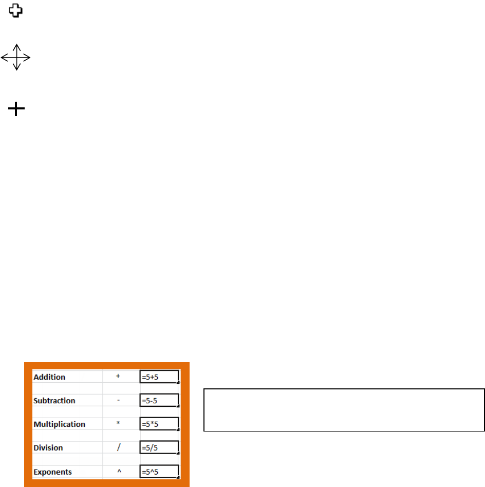
Common mathematical operators in Excel

Advanced Microsoft Excel 2010
Page | 3
Complex Formulas
In the Introduction to Excel class we created simple formulas. In this class we will explore more advanced
equations and functions with absolute and relative cell references.
For complex formulas, try to remember your math teacher’s lesson on the order of operations.
Excel will calculate equations in the following order:
1. Parentheses
2. Exponents
3. Multiplication/Division (whichever comes first)
4. Addition/Subtraction (whichever comes first)
A mnemonic to remember the order of operation is “Please Excuse My Dear Aunt Sally.”
Example:
If the sales tax was 7%, to calculate the total tax in cell
D10, you would enter the formula:
=(D3+D4+D5+D6+D7+D8+D9)*.07
The parentheses tell Excel to calculate the sum of the
items before multiplying the sales tax for the correct
answer of $58.66.
Wrong way:
=D3+D4+D5+D6+D7+D8+D9*.07
In the formula without the parentheses, Excel will
calculate D9*.07 first, then add the rest of the cells. The result of this incorrect tax formula is $819.63.
Relative Cell References in Formulas
So far, we have only used relative cell references in our formulas. They are probably the type of cell references
you will use most often. All cell references are relative by default. In the above café example, the formula
=B3*C3 was used to calculate the total cost of Dark Magic coffee in cell D3. B3 and C3 are relative cell
references. What Excel is actually seeing is two cells to the left of D3 multiplied by one cell to the left. Relative
cell references allow formulas to be easily copied. Instead of copying B3*C3, Excel will know to multiply two
cells to the left by one cell to the left for each cell down the D column.

Advanced Microsoft Excel 2010
Page | 4
Absolute Cell References
Absolute cell references in Excel make it so cells in a formula stay constant once copied, not relative to the
formula’s location. Dollar signs are used to signify an absolute cell reference.
$A$3: The column and the row do not change when copied.
$A3: Column A will not change when copied, but the row
number will change relative to the formula’s position.
A$3: Row 3 will not change when copied, but the column can
change.
Functions
Excel functions are basically pre-designed formulas. In the Introduction to Excel class, we used the AutoSum
and AutoAverage feature – which are in fact functions. There many, many other functions available. Excel also
has a function library where you can search and find various functions.
Insert Function Button
Functions are under the Formulas tab
Search for a function here
Type a description of what you
would like the function to do
and press Enter.
Excel will provide a list of
functions that relate to
your description.
Type a description of what
you would like the function
to do
Excel’s definition of what the
function does

Advanced Microsoft Excel 2010
Page | 5
A function has three different parts:
=ROW(A2)
The argument part of the function typically has a cell range to calculate. The beginning cell reference and the
end cell reference are separated by a colon. Example:
=AVERAGE(A2:A8)
The above function will find the average of the numbers in cells A2 thru A8 (including the numbers in A2 &
A8).
Tip!
If you want row numbers to appear when printed, the ROW function is a useful tool to quickly number rows
The Row function =ROW(A2) will return the number 2 because it is the row number for that cell. You can copy
the function down a column to automatically number rows.
Charts
Charts are great to visually represent data and allow people to interpret meaning quickly.
To insert a chart:
1. Highlight the data to be graphed, including the column and
row titles.
2. Click on the Insert tab.
3. Select the chart type (column, line, pie, etc.).
4. Select the visual style (2-D, 3-D, etc.).
5. The chart will appear on the worksheet.
Chart Design
Once you create a chart, a new group of tabs will appear: Chart Tools -
Design, Layout, and Format. The chart has to be selected in order for
these tabs to be visible.
Equal sign
Function
name
Argument (cell range for
the function to calculate)

Advanced Microsoft Excel 2010
Page | 6
Chart Tools Design Tab
In the Chart Tools Design tab you can:
Change the chart type (see what your data looks like in a pie or line chart instead)
Switch the Row and Column data on the X axis
Do quick layout changes (add a title to the x or y axis, add a legend, show more grid lines, etc.)
Pivot Tables
Pivot Tables allow you to focus in on certain parts of your data to make your spreadsheet more manageable.
In other words, pivot tables summarize data. Only want to view two of your twenty columns? No problem
with pivot tables.
To create a pivot table:
1. Select the table or cells that you want to be the source of the
pivot table’s data.
2. Click on the Insert tab and select the Pivot Table button
3. A Create Pivot Table box will appear confirming the source
spreadsheet of your data. Click OK.
4. A blank Pivot Table will appear on the left and the Field List will
appear on the right.
5. Select what information you would like
shown in your Pivot Table in the Field List.
6. You can also Pivot your data around. What
was once organized in columns can be
switched to the rows. It allows you to look at
your data in a different light.
Blank Pivot Table
Field List

Advanced Microsoft Excel 2010
Page | 7
To Pivot your data:
Pivoting data, or changing the row and column labels, will help you analyze your
data differently.
To change the row or column labels simply click and drag the fields from the Pivot
Table Field List to the Row Label, Column Label, or Sum Value Area like pictured to
the right. To remove the field, click and drag them out of the field list.
You can also create a chart of your Pivot Table (called a Pivot Chart). Select any cell
in your Pivot Table, an Options tab will appear on the ribbon. Click on the Options
tab then Pivot Chart. Updating the Pivot Table will automatically update the Pivot
Chart.
Tip!
If you change any data in the source spreadsheet, the pivot table will NOT
automatically update. To update a pivot table, click on the pivot table, and then go to
Options – Refresh.
For free Excel tutorials:
Go to the website http://www.gcflearnfree.org/office
o There are videos and step-by-step instructions on Excel versions 2000-2016.
Excel Keyboard Shortcuts
Keyboard shortcut
Action
Ctrl + Down or Up Arrow
Moves to the top or bottom cell of the current
column
Ctrl + Shift + Down or Up Arrow
Selects all the cells above or below the current cell
F2
Opens the cell for editing in the formula bar
Ctrl + Home
Navigates to cell A1
Ctrl + End
Navigates to the last cell that contains data
Alt + =
AutoSums the cells above the current cell
Click and drag a field into an area
(row label, column label, value sum)
to change your pivot table.
